A Navigation Algorithm Based on the Reinforcement Learning Reward System and Optimised with Genetic Algorithm

Abstract

Regarding autonomous vehicle navigation, reinforcement learning is a technique that has demonstrated significant results. Nevertheless, it is a technique with a high number of parameters that need to be optimised without prior information, and correctly performing this is a complicated task. In this research study, a system based on the principles of reinforcement learning, specifically on the concept of rewards, is presented. A mathematical expression was proposed to control the vehicle’s direction based on its position, the obstacles in the environment and the destination. In this equation proposal, there was only one unknown parameter that regulated the degree of the action to be taken, and this was optimised through the genetic algorithm. In this way, a less computationally expensive navigation algorithm was presented, as it avoided the use of neural networks. The controller’s time to obtain the navigation instructions was around 6.201·10⁻⁴ s. This algorithm is an efficient and accurate system which manages not to collide with obstacles and to reach the destination from any position. Moreover, in most cases, it has been found that the proposed navigations are also optimal.

1. Introduction

Nowadays, autonomous guided vehicles (AGVs) are expected to be able to accomplish different tasks associated with location estimation, mapping the environment and planning trajectories, navigation and obstacle avoidance. These goals can be achieved with different machine learning algorithms, but reinforcement learning (RL) has proven to be a particularly useful technique for navigation and collision avoidance. This method is associated with the definition of several parameters for its correct performance, and because it is usually arbitrary and of high dimensionality, an additional technique that deals with this task can be useful. Genetic algorithms (GAs) can be a solution, providing more stable systems that are sensitive to small changes in input or noise. Moreover, significant results are achieved as they operate in large multimodal spaces. It is worth mentioning that Q-learning is a reinforcement learning algorithm, but one without a model to learn the action at a specific time, addressing transition and stochastic reward problems.

Within reinforcement learning, an agent interacts with the environment and learns to improve its performance. This enhancement is achieved through the accumulation of rewards, giving it the ability to make decisions in real time. Learning takes place through the Q-networks of the actor and the critic, providing it with a transition model. Regarding navigation tasks performed with the reinforcement learning algorithm, Van et al. [1] generated intelligent navigation in two-dimensional environments, with an algorithm built on a ROS (Robot Operating System) basis, achieving accuracy and efficiency. RL agents can also be trained with Proximal Policy Optimization (PPO), considering deviation errors and being rewarded depending on the agent’s direction (see Sadhukhan et al. [2]). Continuing with the PPO technique, reinforcement learning training can be performed without prior information about the surroundings, as Toan et al. [3] showed by building a convolutional network and adding the Boltzmann policy to generate a trade-off between exploration and harvesting.

Surmann et al. [4] proposed a self-learning test for robots without a map or path planner, considering that, in their words, the models obtained from the RL still suffered from a lack of safety and robustness. In their work, they set the linear and angular velocity of the vehicle as inputs, obtained through an Asynchronous Advantage Actor-Critic network. If laser signals are used in addition to these inputs, it is possible to appreciate how the RL is effective with continuous actions (see Jesus et al. [5]). The problem, therefore, remains in obtaining a satisfactory reward system. When there are objects in the navigation area, it is feasible to orient the vehicle towards them (see Staroverov et al. [6], Staroverov et al. [7]), achieving an optimal algorithm that uses the obstacles as an additional reference to the environment. In this way, low hierarchical levels provide intuition, while high hierarchical levels provide the necessary decisions at each step. Employing equal hierarchical levels, it is possible to provide the agent with accessible reference points for the agent to build a hierarchical policy structure. In other studies, such as Ben Hazem’s [8], the physical model of the system is employed to train the RL agents where an agent training system with Q-learning and deep Q-network learning is used to train data. The actions of the agents are the states of the system and the reward is null in an initial resting state, achieving an effective algorithm as a controller.

Regarding obstacle avoidance, Khriji et al. [9] mention that numerous objects are involved in real-life situations, creating problems in the traditional Q-learning approach. On the one hand, learning Q-values may be unfeasible due to a high memory requirement. On the other hand, rewards may be limited in the environment and would be slow to be obtained. In their study, they propose a reinforcement learning algorithm to coordinate movements, reducing the convergence time of learning. Ribeiro et al. [10] propose two Q-learning views for obstacle avoidance, demonstrating that they can navigate using ROS communication between the control and the robot. The two Q-learning results generate different strategies, enhancing learning and approximating different situations to accomplish the goal. By additionally taking advantage of the storage capacity of Q-learning, the autonomous nature of the AGVs (autonomous guided vehicles) can be guaranteed (see Huang et al. [11]).

In a research study by Duguleana et al. [12], dynamic and static navigation obstacles were avoided in a known working environment. To solve the Q-learning and trajectory problems, they proved that it is possible to use a neural network in conjunction with a planner. Another point of view was proposed by Chewu et al. [13], where they employed the information obtained from simultaneous localisation and mapping (SLAM) so that reinforcement learning could redesign the trajectory to be followed and optimise it. Mohanty et al. [14] decided to add a reward function to deep Q-learning that considered the relative position of the robot, the obstacles and the destination, introducing an algorithm with a high success rate. Wicaksono et al. [15] investigated the use of Q-learning as a learning mechanism to internalise the behaviours of the vehicle during navigation, performing a movement based on the behaviour instead of the surrounding elements.

Genetic algorithms have become a common resource for solving search tasks, with numerous applications in optimisation and guidance problems (see Chakraborty et al. [16]). It is also worth mentioning that they offer significant convergence capability (see Ortiz et al. [17]), which is exploitable for formulating navigable trajectories for AGVs. Al-Taharwa et al. [18] demonstrated in this manner that it is possible to find the optimal trajectory between two points through the GA, thus reducing the number of steps to be taken between both locations. It is also possible to introduce obstacle information (see Tu et al. [19]), with a variable length of the algorithm chromosome, thus conditioning it with the environment. In a study by Santiago et al. [20], it was demonstrated that it is feasible to analyse which set of values is more appropriate depending on the problem, defining the start and end points and penalising encounters with obstacles.

Lamini et al. [21] described an improved crossover driver, enabling them to avoid premature convergence of the algorithm and to achieve trajectories with a higher fitness value than those obtained by the progenitors when generating feasible trajectories. In the study by Tuncer et al. [22], they also focused on preventing such early convergences, as well as keeping the robot from performing unfeasible trajectories, using a new mutation agent. Panda et al. [23] built their study on dynamic behaviour to approach the dynamic motion planning problem as a trajectory planning and control task of the integrated system. Furthermore, they mentioned that the dynamic motion planning problem could be converted into an optimisation problem in the acceleration range of the robot.

Jafaf Jalali et al. [24] demonstrated that the genetic algorithm was useful to find the optimal architecture of a deep neural network based on hyperparameters, and to perform their study, they applied it to training for the navigation of an autonomous vehicle. Kumar et al. [25] analysed the robot motion task using linear regression along with genetic algorithms to design the vehicle controllers. The GA-based controller was concerned with calculating the best successive position of the AGV based on the distance to the nearest obstacle. In addition, they implemented a Petri net for obstacle avoidance. In the case of the investigation by Yoshikawa et al. [26], a three-part system was presented in which, on the one hand, a technique that combined the GA and the Dijkstra algorithm to achieve a quality route was presented, and on the other hand, the navigation system complied with position landmarks. Finally, new agents were introduced that did not allow a lethal gene to be generated. It should be noted that the task assignment of an AGV defines the scheduling process of this one, considering the waiting times of the tasks (see Mousavi et al. [27]), so the scheduling of a robot with different positional targets became a complex and combinatorial problem.

With the environment in focus, Gyenes et al. [28] analysed whether a genetic algorithm could avoid obstacles in real time during navigation. For this purpose, they created a family of algorithms combining GA and obstacle velocity models, demonstrating that suitable performance could be achieved with an appropriate parameterisation of the chromosomes. Kwaśniewski et al. [29] mentioned that for cases where there are obstacles in the environment, solutions based on graph algorithms consume a large amount of computational power. They also pointed out that neural networks or fuzzy logic performed poorly in complex environments. In their study, they relied on a two-dimensional map to compute the path model, which can be different in the same map due to the arbitrary nature of the GA. Sedighi et al. [30] relied on local obstacle avoidance, where in addition to finding a valid trajectory, they also aimed for an optimised route. In search of such optimisation, Geisler et al. [31] described the development of software that relies on genetic algorithms. In this paper, they proposed a new coding technique developed to optimise the GA information. Another study aimed at obstacle avoidance was presented by Ghorbani et al. [32], this time applying the GA to a global environment. To reduce the complexity, they proposed converting the two-dimensional encoding of the waypoint points into a one-dimensional encoding. In this way, they managed to integrate the ability to avoid obstacles and find the shortest distance to the destination into one function.

Several studies focused on investigating improvements in reinforcement learning algorithms could successfully execute robotic navigation in dynamic environments (see Yen et al. [33]). For instance, the inclusion of forgetting mechanisms or the use of a hierarchically structured RL agent was shown to provide superior performance. Moreover, it is recognised that deep artificial neural networks (DNNs) are often trained with learning algorithms that are based on gradients. In this case, evolutionary strategies can compete with these algorithms in complex reinforcement learning problems, as highlighted by Such et al. [34]. Evolutionary algorithms, moreover, can be considered stochastic gradient descent-based algorithms since they operate similarly to a finite-difference approximation of the gradient. Therefore, it is possible to show that the weights of a DNN can be evolved with a simple, gradient-free GA that works on deep RL problems.

Assuming that improvements can be generated, numerous studies have tried to combine both strategies, GA and RL. It is also recognised that the selection of the parameter values of the RL algorithm can significantly affect the learning process, so it is also possible to use the GA to find the values and assist the agent in learning, achieving high performance (see Sehgal et al. [35]). Kamei et al. [36] also mention that it is possible to avoid supervised signals in the RL framework, making it suitable for obstacle-avoidance navigation of mobile robots, although they also point out the algorithm’s value determination without prior information. They propose the use of a genetic algorithm with inheritance for the optimisation of these, managing to reduce the number of actions needed by the vehicle to reach the target position, achieving shorter paths. They also demonstrate that the learning speed can be reduced by keeping the number of necessary actions low (see Kamei et al. [37]).

Stafylopatis et al. [38] discuss that in general, RL schemes perform online searches in the control space, making them suitable algorithms for improving system performance due to the possibility of control rule modification. In their study, they verified this suitability by training a learning classifier system (LCS) that controls vehicle motion. They composed the system with a set of condition–action rules that evolved with a GA, conditioning the evolution with rewards and obtaining superior performance to other techniques on the same problem. In reactive control systems, Ram et al. [39] proposed evolution in diverse environments, creating sets of what they called ‘ecological niches’ that can be used in similar environments. Thus, using GA as an unsupervised learning method reduces the effort to set up a navigation system. When navigation is performed in previously unmapped environments, genetic deep reinforcement learning (GDRL) approaches can be considered, in which GA approaches are combined with discrete and continuous action space deep reinforcement learning (DRL) (see Marchesini et al. [40]), thus reducing the sensitivity of RL approaches to hyperparameter tuning and generating robust strategies.

On the other hand, genetic network programming with reinforcement learning (GNP-RL) has important features over other evolutionary algorithms, such as the combination of offline and online learning or the combination of diversified and intensified search (see Findi et al. [41]), and it is generally used to navigate in static environments. For dynamic environments, therefore, the problem of determining smooth and collision-free trajectories that can be navigated quickly can be addressed with a GNP-RL based on collision position prediction, generating safe navigation. Sendari et al. [42] proposed GNP-RL programming, including conventional fuzzy logic with fuzzy judgment nodes. In this way, they provided flexibility in choosing the next appropriate node by probabilistic transition, thus generating more robust systems.

The principal purpose of this study is the development of a navigation algorithm for the AGV which can be seen in Figure 1. This vehicle was built by Argolabe Ingeniería, SL, a company located in Vitoria-Gasteiz, Spain. This algorithm was initially designed for simulation, meaning that it is intended to operate in a two-dimensional (2D) indoor environment. Furthermore, it must have the ability to avoid collisions. For this purpose, the research is based on the principles of reinforcement learning, specifically the concept of rewards, and combines it with genetic algorithms for the determination of the optimal values of the designed algorithm. Hence, the designed algorithm must be able to calculate a feasible trajectory to a target point in a specific environment using a series of mathematical operations, ensuring the integration and coexistence of both techniques. In this way, a concept similar to RL is presented, since the control system is evaluated in the same way as in RL, but the system to be adjusted—in other words, the controller—is considerably simpler.

For this objective, the article first presents the dynamics of the vehicle’s movement, which gives place to the control law. With this control law, the importance of the fulfilment of the objectives is also regulated and translated into a mathematical expression. Therefore, both dynamics and control are included in a single mathematical relation, which must be optimised, this being the main contribution of the work. This equation calculates the action that the vehicle will take—in other words, in which direction it has to go to reach its destination and avoid collision. As it is a single expression, the control of the autonomous vehicle is simplified. This formulation incorporates a variable named $K$ that is optimised through the genetic algorithm, being an adaptable value if necessary due to the characteristics of each environment. Therefore, it provides robustness to the algorithm as well as flexibility. Only the concept of reinforcement learning rewards is used so that an algorithm without the use of neural networks is presented, thus providing a lower computational cost. In this way, it can obtain the necessary commands for the vehicle to perform the navigation, and this can be performed both offline and online.

2. Materials and Methods

This study introduces an algorithm for the indoor navigation of an autonomous guided vehicle. Autonomous vehicles require a control algorithm to reach the desired destination by generating optimal navigation. Furthermore, this navigation must avoid collisions between the vehicle and obstacles in the environment. In this study, the starting point is the concept of reinforcement learning, in which the control system is evaluated through rewards. Only this idea is taken, that of evaluating through rewards, but a simpler controller with less computational effort is generated. A mathematical expression (Equation (24)) is proposed to operate as a controller. For each instant of time, it must calculate the necessary instructions for the movement of the AGV, taking into account the distance to the target and the distance to the obstacles. This mathematical expression is optimised through the genetic algorithm, being suitable for each navigation situation.

A flow chart that clarifies the process is presented in Figure 2. Initially, the proposed mathematical expression is taken. This equation has a parameter $K$ to optimise, and a value for this parameter is proposed through the genetic algorithm. With this value substituted in the mathematical expression of the controller, the plant and the environment are considered and navigation is simulated. In this way, it is possible to calculate the reward that has been generated in each of the movements made by the vehicle. $Q$ refers to the accumulated reward over the entire trajectory, in other words, the sum of the value of the reward achieved at each step. This $Q$ value is evaluated using the genetic algorithm, which proposes a new value of $K$ until the value of $Q$ is maximised.

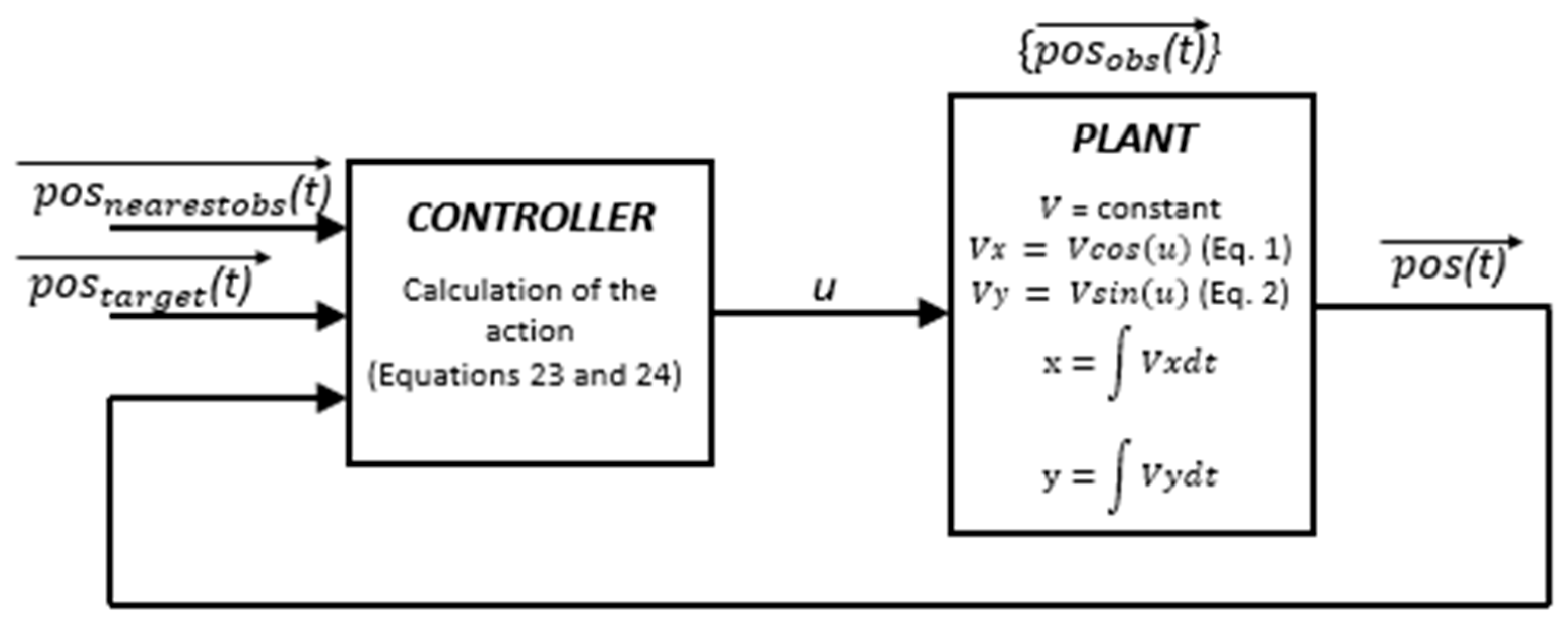
To clarify the functionality of the controller, Figure 3 is presented, with a flow chart describing its operation. Initially, the controller considers the current position of the vehicle $\overrightarrow{pos\left(t\right)}$, the target position $\overrightarrow{{pos}_{target}\left(t\right)}$ and the position of the nearest obstacle ($\overrightarrow{{pos}_{nearestobs}\left(t\right)}$). With this information and through the proposed mathematical expression, an action value is calculated, defined as $u$. Considering the positions of the set of obstacles in the environment $\overrightarrow{\left\{{pos}_{obs}\right(t\left)\right\}}$ and also knowing that the speed at which the vehicle will navigate is constant, the next position it will reach is calculated.

For this controller to be effective, as mentioned above, the action will be a function that depends on the current position of the vehicle $\overrightarrow{pos\left(t\right)}$, the target position $\overrightarrow{{pos}_{target}\left(t\right)}$ and the position of the nearest obstacle $\overrightarrow{{pos}_{nearestobs}\left(t\right)}$, plus the parameter $K$ which will be the optimised value, as depicted in Equation (1).

$$u\left(t\right)=f(\overrightarrow{pos\left(t\right)},\overrightarrow{{pos}_{nearestobs}\left(t\right)},\overrightarrow{{pos}_{target}\left(t\right)},K)$$

(1)

To decide the best value of $K$, it is proposed to maximise the value of the reward obtained during the entire navigation, which is the sum of all the rewards generated with each proposed step during the trajectory. These values depend on the current position and the calculated action, as shown in Equation (2).

$$Q=\sum _{t=0}^{t=N}reward(\overrightarrow{pos}\left(t\right),u\left(t\right))$$

(2)

About the code of both flow charts, the pseudocodes are shown below. In the first Algorithm 1, what would be the main execution is shown. Therefore, first, the global variables such as the map, the position of the obstacles and the destination position are defined. Then, the parameters with which the GA will optimise the desired value are set. In addition, it is necessary to define how much importance is to be given to reaching the destination and not colliding with obstacles in the environment (see Equation (12)). Once this has been defined, the control algorithm is executed, which is set out in a function as shown in Algorithm 2, in such a way that the optimum value of $K$ is searched for as described in the flow chart in Figure 1. When the optimum value of $K$ is obtained, the controller function is executed again (see Algorithm 2), but with this value as a fixed input, navigation is carried out.

Algorithm 1.  Pseudocode of the algorithm’s operation
MAIN: Execution of the Navigation Algorithm
1:	Definition of global variables (map and obstacles, target position)
2:	Definition of values for GA implementation
3:	$\mathrm{Definition}\mathrm{of}\mathrm{the}\mathrm{degree}\mathrm{of}\mathrm{importance}\mathrm{of}\mathrm{meeting}\mathrm{targets}{\alpha }_1$  $\mathrm{and}{\alpha }_2$
4:	Call to the function with a range of K to optimise it with the GA
5:	Function call again with optimised K value to generate navigation

For the pseudocode in Algorithm 2, the inputs are the value of $K$, the position of the destination and obstacles and the map of the environment. The output will be the value of the reward plus the parameters necessary for the vehicle to perform the navigation. First of all, the starting position from which the AGV will start is defined. In addition, the speed of the AGV, the integration step and the number of iterations are set. With this information, a loop is generated which will end when the desired position is reached. In this loop, the relative distance between the current position of the vehicle and the target position is first obtained (see Equation (16)). The distance from the AGV to all obstacles is calculated to find out which is the closest obstacle, and the relative distance to this obstacle is calculated (see Equation (17)). With this information, the alignment angle of the vehicle to the destination can be estimated (see Equations (18) and (19)). A change of coordinates from the absolute reference system to the vehicle reference system is performed with a matrix (see Equation (20)) so that the next relative desired position that the vehicle should reach can be calculated (see Equations (21) and (22)). The action required to reach that position is calculated (see Equations (23) and (24)) and the move is made (see Equations (8) and (9)). With this, the reward value generated in that step can be calculated (see Equation (12)). Once the target position is reached, the accumulated reward for the entire navigation is calculated (see Equation (15)). Finally, the graphs, reward and $K$-values are obtained, which can be seen in Section 3.

Algorithm 2. Pseudocode of the function performing navigation with designed mathematical equation
Function: Execution of the Navigation Algorithm (In: K, Obstacles and Target Position, Environment/Out: Reward, Navigation Parameters)
1:	Definition of starting point of navigation
2:	Definition of values for max speed, time steps, number of iterations
3:	$\mathrm{for}t\leftarrow$ Number of iterations
4:		Obtain the relative distance from the current position to the finish point
5:		Obtain distance to all obstacles and keep the nearest one
6:		Obtain the relative distance from the current position to nearest obstacle
7:		Calculate the required alignment angle
8:		Generate the coordinate change matrix with the angle of alignment
9:		Calculate the next position that the vehicle should reach with the matrix
10:		Calculate the action needed to reach that next position
11:		Move forward
12:		Calculate value of reward that has been generated by the movement
13:		Draw trajectory realised by the AGV
14:	end
15:	Calculate cumulative reward value

In this way, with a simple code, it is possible to carry out optimised navigation for an autonomous vehicle and to evaluate the generated reward.

2.1. Vehicle Dynamic Model

To design the programming of the robot, it is necessary to take into account its dynamics to obtain the command for its operation. These instructions will be used to indicate to the robot at which speed it has to go and which direction it has to follow. As can be appreciated in Figure 1, the robot has a motor that actuates two wheels, so the speed command indicates how fast the wheels have to rotate and the rotation is carried out by giving more speed to one wheel than to the other.

Consequently, it can be considered that two linear velocities are involved: the linear velocity on the x-axis and the linear velocity on the y-axis of the navigation environment, $V_x$ [m/s] and $V_y$ [m/s] (see Figure 4), respectively. Furthermore, both form a vector which will be the linear velocity $V$ [m/s] that determines the direction adopted by the autonomous vehicle. This direction is also clearly influenced by the direction taken by the vehicle itself, corresponding to the angle of rotation ${\vartheta }_v$ [rad]. The latter indicates that the robot can rotate around itself. This means that the vehicle is capable of translational and rotational movements. The transformations of the coordinate systems for the velocities are defined as in Equations (3) and (4), taking into account that $t$ refers to the time instant:

$$V_x\left(t\right)=V\left(t\right)\cos \left({\vartheta }_v\left(t\right)\right)$$

(3)

$$V_y\left(t\right)=V\left(t\right)\sin \left({\vartheta }_v\left(t\right)\right)$$

(4)

Therefore, the set points that the vehicle mainly needs for navigation are the linear velocity $V$ [m/s] and the angle of rotation ${\vartheta }_v$ [rad].

Collecting the values described in Figure 4, a vector of actions $\overrightarrow{u}$ is defined which collects these values, as shown in Equation (5). Moreover, this vector is applicable at any time instant of the navigation.

$$\overrightarrow{u}\left(t\right)=[V_x\left(t\right),V_y\left(t\right),{\vartheta }_v(t\left)\right]$$

(5)

Table 1. Dynamic parameters affecting the autonomous vehicle.

Parameter	Description	Unit
$V_x$	Linear velocity on the x-axis	[m/s]
$V_y$	linear velocity on the y-axis	[m/s]
$V$	Linear velocity	[m/s]
${\vartheta }_v$	Angle of rotation	[rad/s]
$\overrightarrow{u}$	Vector of actions	-

below lists the parameters defined in this section for a more direct visualisation of them.

With the parameters that are going to act on the vehicle defined, it is necessary to establish the control law that it is going to follow, giving the possibility of identifying the positions that the vehicle is going to achieve in future instants.

Vehicle Control Model

Knowing the parameters which act on the mobile robot, it is necessary to formulate their control law to be able to identify the positions of the mobile robot in the future states. For this purpose, the following Equations (6) and (7) are proposed, where $x$ [m] and $y$ [m] refer to the positions of the vehicle in the plane. In addition, another parameter defining the integration step is included with the notation $∆t$ [s]. Since the velocities are being considered per axle individually, the same has to be done for the positions. The step function is thus described.

$$x\left(t+1\right)=x\left(t\right)+u_1\left(t\right)∆t$$

(6)

$$y\left(t+1\right)=y\left(t\right)+u_2\left(t\right)∆t$$

(7)

As mentioned already, the set points have to be the velocity $V$ and the angle ${\vartheta }_v$, so Equations (6) and (7) are rewritten considering these parameters (see Equations (3) and (4)), as presented in Equations (8) and (9).

$$x\left(t+1\right)=V\left(t\right)\cos \left(u_3\left(t\right)\right)∆t$$

(8)

$$y\left(t+1\right)=V\left(t\right)\sin \left(u_3\left(t\right)\right)∆t$$

(9)

The control law to be used by the AGV is defined with these equations, allowing the development of the navigation algorithm, since the values that need to be obtained can be determined. To simplify the development of the algorithm, the speed value is set at $V=1$ [m/s] and the integration step $∆t=0.5$ [s]. In this way, the algorithm operates on obtaining the values of the vector $\overrightarrow{u}\left(t\right)$ defined in Equation (5). Furthermore, by defining these constants and using Equations (8) and (9), the only value that is necessary to calculate corresponds to the angle of rotation, $u_3\left(t\right)$, which will be identified as the action to be taken.

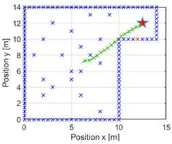
The objective of the proposed navigation is simple. The autonomous vehicle has to navigate around the map reaching a destination point, as well as avoiding collisions with obstacles it may encounter in the environment. This being so, the map in Figure 5 is proposed. The figure shows a bounded area, and therefore it is understood that the walls that delimit the area are considered obstacles and are represented by blue crosses. Since an optimisation is being sought, in the first instance, no further obstacles are considered within the navigation area. The target position is set at $[12.5,12]$ [m] on the map and is represented by a red star.

It has been mentioned that there are two main goals, the first one being to reach the destination and the second one to not collide with the surrounding objects. In this way, Equations (10) and (11) can be defined, which consider the distance from the instantaneous position of the vehicle to the destination ${dist}_{target}\left(t\right)$ or to the nearest obstacle ${dist}_{obs}\left(t\right)$. Both are performed with the Euclidean norm.

$${dist}_{target}\left(t\right)=norm\left(\left[x_{target},y_{target}\right]-\left[x\left(t\right),y\left(t\right)\right]\right)$$

(10)

$${dist}_{obs}\left(t\right)=norm\left(\left[x_{obs},y_{obs}\right]-\left[x\left(t\right),y\left(t\right)\right]\right)$$

(11)

In order to develop the navigation algorithm, the idea of rewards, which are the basis of reinforcement learning, is considered first. It is known that in reinforcement learning, an agent interacts with the environment and thereby learns to improve its performance through the accumulation of rewards. In this way, it is able to sequentially make decisions in real time.

Consequently, the function $reward\left(t\right)$ should consider both parameters defined in Equations (10) and (11). In addition, each assignment is evaluated differently, giving more importance to not colliding with obstacles. Thus, the constants ${\alpha }_1=20$, which is associated with the importance of reaching the destination, and ${\alpha }_2=100$, which gives more importance to avoiding collisions, are defined. Equation (12) is therefore determined.

$$reward\left(t\right)={\alpha }_1{\left({\displaystyle \frac{1}{{dist}_{target}\left(t\right)}}\right)}^2+{\alpha }_2{\left({dist}_{obs}\left(t\right)\right)}^2$$

(12)

To simplify the mathematical notation, the position vector of the AGV is defined, in which the spatial positions of the AGV on the map are collected and defined as $\overrightarrow{pos}\left(t\right)=\left[x\left(t\right),y\left(t\right)\right]$. In the case of the action vector $\overrightarrow{u}\left(t\right)$, it continues to represent the action, but due to the aforementioned simplifications, it now only collects a single value, being $u\left(t\right)={\vartheta }_v\left(t\right)$. As mentioned, the velocity is constant, so continuing to consider the whole vector is meaningless. This way the action is achieved, being the necessary information needed by the vehicle to reach the subsequent position.

2.2. Design of Mathematical Expression for Action Calculation

Certain elements need to be considered in reinforcement learning. On the one hand, the set of states can be defined as $s\left(t\right)$. It is also necessary to define a set of actions, known as $a\left(t\right)$. In addition, a transition function, defined as $T$, is necessary, together with the reward function $reward(s,a)$, which depends on the states and actions to determine the value of the reward. Generally, reinforcement learning is performed through the neural networks of the actor $\pi$ and the critic $Q$, giving them a model. In this way, the next state will have the value shown in Equation (13) below, where $a\left(t\right)=\pi \left(s\left(t\right)\right)$.

$$s\left(t+1\right)=T\left(s\left(t\right),\pi \left(s\left(t\right)\right)\right)$$

(13)

The reward is instead calculated purely with the critic’s neural network, as seen in the following Equation (14), where $\gamma$ is a discount factor.

$$\gamma reward\left(t\right)=Q\left(s\left(t\right),\pi \left(s\left(t\right)\right)\right)$$

(14)

Instead of employing the critic as a neural network, it is stated as a function to save computational cost. Since a mathematical expression is to be used, the objective of this is therefore to maximise the reward value to obtain the highest value of the critical. This function is defined in Equation (15), where $N$ corresponds to the number of iterations. It should be noted that the value of the critical will be unitless. In this equation, it can be considered that the actual position of the vehicle together with the instantaneous action will correspond to the position that the robot will adopt in the following instant.

$$Q=\sum _{t=0}^{t=N}reward(\overrightarrow{pos}\left(t\right),u(t))=\sum _{t=0}^{t=N}reward(\overrightarrow{pos}\left(t+1\right))$$

(15)

It can also be noted that the target position and the nearest obstacles have their own $x$ and $y$ values, and in the same manner as with the position of the vehicle, they can be collected in vectors, named $\overrightarrow{target}=\left[x_{target},y_{target}\right]$ and $\overrightarrow{Obs}=\left[x_{obs},y_{obs}\right].$Using these values, the relative position between the robot and the target ${\overrightarrow{postarget}}_{rel}$ and between the vehicle and the nearest obstacle ${\overrightarrow{posObs}}_{rel}$ can be calculated. Both calculations can be seen in Equations (16) and (17).

$${\overrightarrow{postarget}}_{rel}(t)=\overrightarrow{target}-\overrightarrow{pos}\left(t\right)$$

(16)

$${\overrightarrow{posObs}}_{rel}(t)=\overrightarrow{Obs}-\overrightarrow{pos}\left(t\right)$$

(17)

Having obtained these data, it is possible to calculate the alignment error between the instantaneous position of the vehicle and the target. Therefore, it was decided to define the relative position towards the target as a complex number $Z$ (see Equation (18)) on the x-axis of the environment where the real numbers are going to be found, with the imaginary ones being on the y-axis.

$$Z=x_{{postarget}_{rel}}\left(t\right)+i{y}_{{postarget}_{rel}}\left(t\right)$$

(18)

This way, Equation (19) is proposed in which the angle of alignment of the vehicle ${\vartheta }_{alig}$ is calculated, that is, the orientation that it should adopt. For this purpose, the notation of the $Z$ value is changed by converting it from a complex number to a polar number with the relation $Z=r_{\angle \vartheta }$ and preserving the angle of this value.

$$angle\left(r_{\angle \vartheta }\left(t\right)\right)={\vartheta }_{alig}\left(t\right)$$

(19)

Continuing with the value of the alignment angle, the matrix $M$ of Equation (20) is established. This matrix is used in order to be able to change the reference system from an absolute system to that of the vehicle.

$$M(t)=\left(\begin{array}{cc}\cos \left({\vartheta }_{alig}\left(t\right)\right)& -\sin \left({\vartheta }_{alig}\left(t\right)\right)\\ \sin \left({\vartheta }_{alig}\left(t\right)\right)& \cos \left({\vartheta }_{alig}\left(t\right)\right)\end{array}\right)$$

(20)

With the support of this matrix, Equations (21) and (22) are defined, which are used to estimate the relative positions that the vehicle will take concerning the goal and the nearest obstacle.

$${\overrightarrow{postarget}}_{rel}(t+1)=M\left(t\right){\overrightarrow{postarget}}_{rel}\left(t\right)$$

(21)

$${\overrightarrow{posObs}}_{rel}(t+1)={M\left(t\right)\overrightarrow{posObs}}_{rel}\left(t\right)$$

(22)

Based on this information, the calculation of the value of the action $u\left(t\right)$ is proposed. In case the subsequent position to be reached by the vehicle is directed towards the target point, the value of the action will be in a range between $[-\pi ,\pi ]$, always considering the relative position towards the goal. Moreover, in this way, if the target position is aligned with an obstacle, it will not be necessary to change the direction as long as the obstacle is at the back of the vehicle. Thus, the value of the action is computed with Equation (23).

$$u\left(t\right)=\mathrm{atan}\left({\displaystyle \frac{y_{{postarget}_{rel}}\left(t\right)}{x_{{postarget}_{rel}}\left(t\right)}}\right)$$

(23)

Otherwise, that is, if there is a need for a deviation, a correction term will be added to Equation (23), assuming values in the range of $[-{\displaystyle \frac{\pi }{2}},{\displaystyle \frac{\pi }{2}}]$. In this situation, the next estimated position to be reached will be considered, both concerning the goal and concerning the nearest obstacle. In addition, a new unitless parameter $K$ is incorporated, which will multiply this correction. This adjustment is described in Equation (24).

$$u\left(t\right)=\mathrm{atan}\left({\displaystyle \frac{y_{{postarget}_{rel}}\left(t\right)}{x_{{postarget}_{rel}}\left(t\right)}}\right)+\mathrm{atan}\left(K\left(\left(x_{{posObs}_{rel}}\left(t+1\right)-x_{{postarget}_{rel}}\left(t+1\right)\right){\displaystyle \frac{x_{{posObs}_{rel}}\left(t+1\right)}{y_{{posObs}_{rel}}\left(t+1\right)}}\right)\right)$$

(24)

2.3. K-Optimised Parameter Search with the Use of Genetic Algorithm

The genetic algorithm becomes relevant in this stage, where it will be employed to evaluate the impact of this correction; in other words, it will be used to optimise the value of the $K$ parameter. In addition, to facilitate the search for the GA, it will be restricted so that $K$ can only obtain values between $0.01$ and 1. Furthermore,

Table 2. Genetic algorithm configuration parameter.

Parameter	Value
Constraint Tolerance	1 × 10−6

shows the additional parameters that have been set for the search performed by the genetic algorithm.

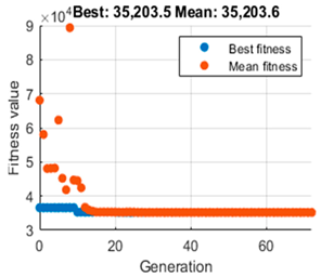
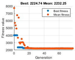
The constraint tolerance value establishes the feasibility concerning nonlinear constraints. However, there is a second value that may generate different agents and, therefore, more appropriate navigation. This is the value of the population size, which defaults to 50 for problems with five or fewer variables to optimise.

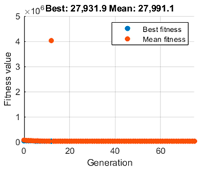
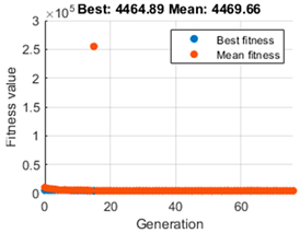
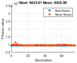
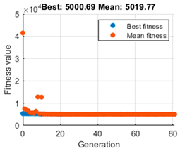
As mentioned, there is only one parameter to optimise, $K$, and additionally, the evolution graph of the GA algorithm gives us information on the maximum reward accumulated during the whole trajectory and the average. To make a comparison and decide which is the most appropriate population value,

Table 3. Comparison of AG performance for appropriate population search.

GA Performance	Generated Navigation	Execution Information
		$Population=50$ $Q=\mathrm{27,931.1}$ $Time=1.697 \mathrm{s}$ $K=0.0463$
		$Population=25$ $Q=\mathrm{27,931.1}$ $Time=1.1362\mathrm{s}$ $K=0.0463$
		$Population=10$ $Q=\mathrm{35,203.5}$ $Time=0.694\mathrm{s}$ $K=0.1002$
		$Population=5$ $Q=\mathrm{27,931.9}$ $Time=0.5775\mathrm{s}$ $K=0.0464$

is presented. It shows on the left the evolution of the GA algorithm in its search for the optimal value, which depicts the fit value taken by each generation. The red dots indicate the best fit achieved by each epoch, while the blue dots show an average of these fits. In the central part, the simulation of the navigation is performed with the $K$ parameter defined. Finally, on the right, the selected population data $Q$, the time required by the GA algorithm for the search and the value of $K$ in each case are presented. All this is for the map presented in Figure 5. The vehicle is positioned at the starting point $\left[\mathrm{1,1}\right]$ [m] for this test. It is worth mentioning that the execution stops when the vehicle is $0.3$ m away from the destination point. Furthermore, red crosses can be seen in the graphs illustrating the navigated trajectory, referring to the closest obstacle detected in the last iteration. In the case of the green crosses, they indicate the position reached in each iteration. Since it is talking about times, it is worth mentioning that Matlab R2023b was used to carry out the simulations, with a computer with a 13th Gen Intel(R) Core(TM) i5-1335U 1.30 GHz processor and a RAM of 16 GB.

The left column, as mentioned above, shows the performance of the genetic algorithm in finding the optimal value of $K$ that maximises reward. More significant, however, are the middle column and the data on the right. In all cases, it can be seen that the vehicle can perform navigation that reaches the target.

As for the tests with a population size of 50 and 20, it can be appreciated that although the performance of the GA is different, the same trajectory is obtained. Moreover, both the cumulative reward value and the optimal value of $K$ coincide with the difference that the population of 20 needs less time to search for the desired optimal parameter. By paying attention to the trial with a population size of 5, the GA algorithm can quickly refine the optimal value of $K,$ as shown in the graph on the left. The value of the cumulative reward can also be considered equal to that achieved with the population size of 20 and 50, and the navigation path is equal. The most significant difference is in the time elapsed to achieve the value of $K$, which is much shorter, so the 20 and 50 population size options were discarded.

Comparing the tests with a population size of 10 and a population size of 5, it can be observed at first glance that the navigation proposed by the population size of 10 is not the most optimal and that it performs a curve that should not necessarily be so sharp. Moreover, it can be noticed that the value of $Q$ is higher in this case, as well as the value of $K$ calculated. Nevertheless, the speed of calculation of the population size of 5 is prioritised and the generated trajectory is considered to be more optimal and navigable.

Accordingly, the population size of 5 was chosen for the GA, and this evolution provides an optimal value of $K=0.0464$. Once the required action is achieved, the actual next step to be performed by the vehicle is estimated, as defined in Equations (8) and (9). The actual next step is calculated as many times as necessary until the target is completed. The value of the reward can be calculated with the help of Equation (15), and by accumulating the value of the reward to be obtained in all steps, it is also possible to calculate the value of the critical, which in this case is $Q=\mathrm{27,931.9},$ achieving the maximisation of the reward.

3. Results

To verify the correct performance of the algorithm, it was first tested in a simplified environment, to which obstacles were then added. It should be recalled that a population size of 5 had already been determined in the genetic algorithm, so it was a constant parameter in obtaining the results.

3.1. Result in an Area Without Intermediate Obstacles

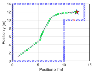
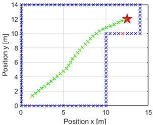
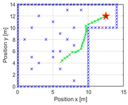
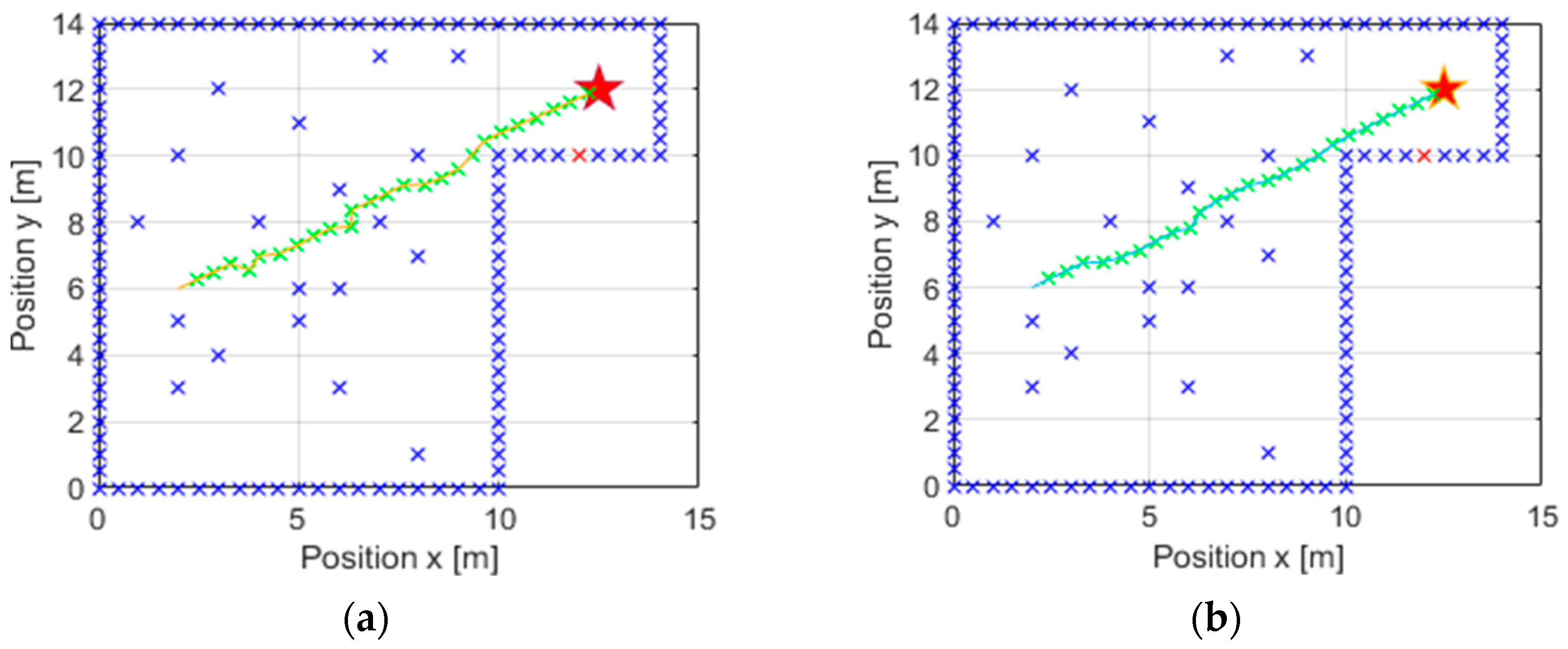
Values obtained with the development of the previous section were tested on the map presented in Figure 5. The vehicle was positioned at the starting point $[1,1]$ [m] and the navigation simulation was started by setting $N=1000$ iterations, which would be interrupted once the target had been reached. This resulted in a navigation with the trajectory depicted in Figure 6. In addition, the green crosses indicate the position that the vehicle will take in each instant, and it may be seen that an obstacle is now coloured red, indicating the nearest obstacle in the direction of the vehicle. It should be recalled that the value of $K$ was limited between $0.01$ and $1$ for this execution.

To better appreciate this, Figure 7 is presented, in which the most representative areas of Figure 6 are enlarged. In the image on the left, it can be observed that at the beginning of the navigation, the action did not change and continued straight ahead without modifying the value of the action required. In the central image, it can be seen that it had recognised that an obstacle would get in the way if it continued with the same action value, so it applied a correction to the turn. In addition, once it no longer detected that obstacle in the way, it continued correcting the direction to head towards the goal. In the image on the right, it finally arrived at the destination, but we can appreciate how the correction of the action was more significant to reach the desired point.

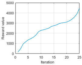
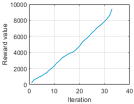
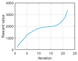
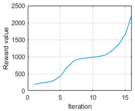
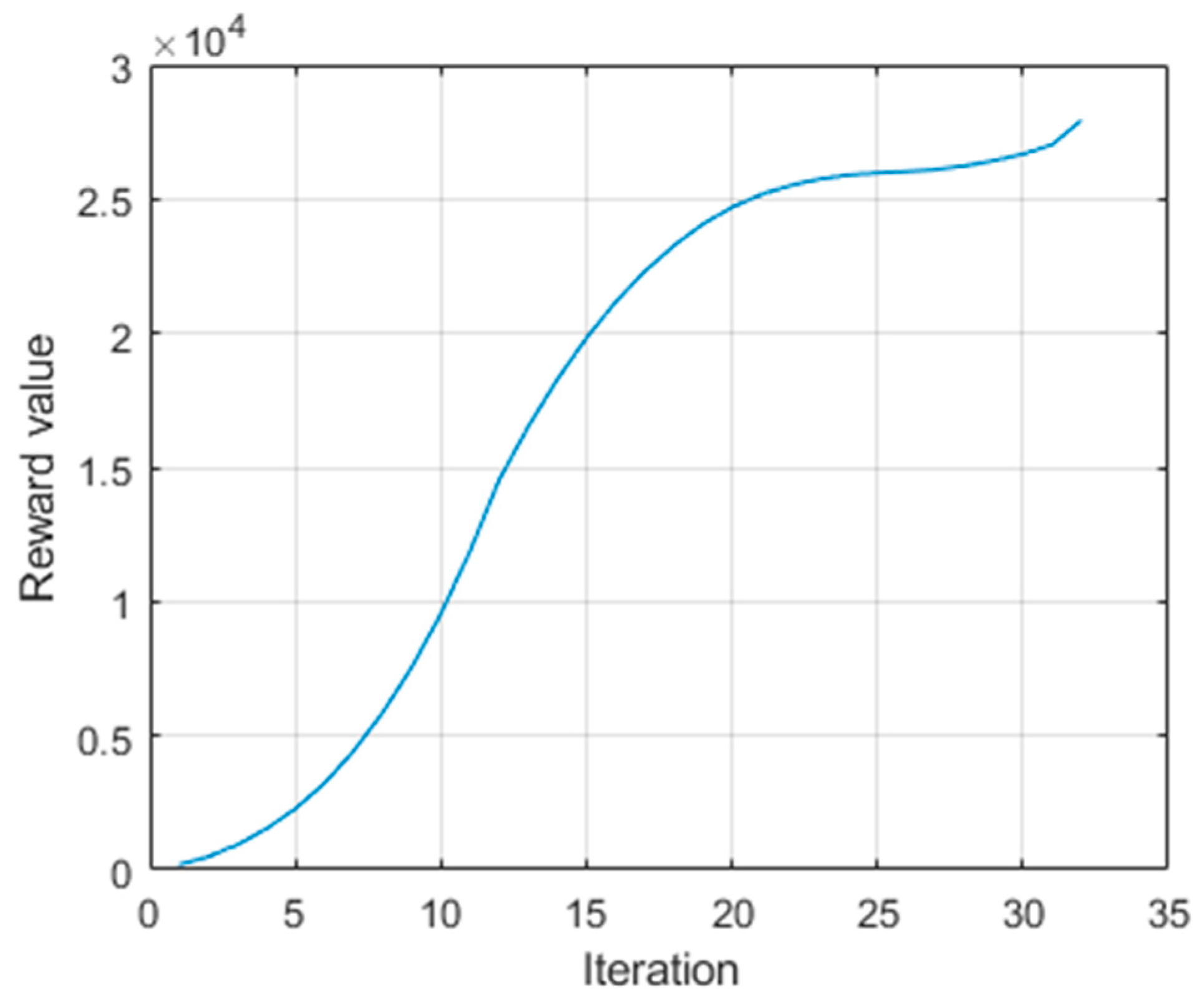
It is possible to appreciate how the complete trajectory from the initial point to the target can be estimated using this approach. In this way, it is possible to navigate in an environment without colliding with obstacles as a result of the action optimised by the genetic algorithm. As a fact, the reward value obtained in this trajectory is $Q=\mathrm{27,931.9}$. Figure 8 is presented to represent the evolution of the reward. It is worth noting that the vehicle needed $32$ iterations to reach the destination and that it travelled a distance of $16$ m. Furthermore, the execution of the controller was completed in $0.0014$ s.

Figure 8 shows that at the beginning of the iterations, it did not accumulate many rewards, as it did not encounter obstacles and the arrival at the target was less evaluated (see Equation (12)). When it detected that by continuing along this path, it would come across an object, it accumulated more reward value, increasing the curve. Finally, as it reached the target, the value added was lower.

In this way, it can be verified that in addition to reaching the target and avoiding obstructions, it is possible to generate optimal navigation. When calculating the linear distance between the initial point and the target point, the result obtained is $15.9138$ m. It has been mentioned that the distance travelled by the vehicle to reach the destination is $16$ m, so the deviation generated has meant less than $0.1$ m of extra distance, which is necessary to avoid the obstacle and thus justify optimal navigation.

3.2. Results in an Area with Intermediate Obstacles

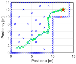
Having performed the initial verification in an environment where the obstacles were only in the margins of the area, the efficiency of the algorithm was tested in the same environment, but with obstacles placed around it, as can be seen in the map shown in Figure 9.

The following figures in

Table 4. Different paths calculated in an obstacle environment.

Test	GA Performance	Generated Navigation	Cumulative Reward
1.
2.
3.
4.
5.
6.

represent different navigations performed by the robot with varying starting points. Each line represents a performance of the algorithm, starting the navigation from a different point on the map. On the left is shown the performance of the genetic algorithm in search of the parameter $K$ to be optimised. In the centre are shown the trajectories of the navigations, while on the left are displayed the graphs of the reward that accumulated during the execution of the navigation. It should be remembered that all these tests were conducted by limiting the search for the value of $K$ to between $0.01$ and $1$.

In the images above, it is evident that regardless of the starting point of the navigation, the vehicle can reach the goal on all occasions. The proposed design was also capable of avoiding collisions in all the experiments carried out, so it can be concluded that it fulfils the two main objectives established. A more exhaustive analysis of the performance of the genetic algorithm shows that in all cases, it already managed to minimise the fit value for generation 20. Furthermore, it is noteworthy that in tests 2, 3 and 4, this was achieved practically immediately. With this, it can be stated that the genetic algorithm performs adequately when searching for the appropriate $K$ parameter for each case.

Once this parameter has been determined, and moving on to the central column, the navigation column, different trajectory shapes can be seen. The first case corresponds to the longest trajectory, and in this case, it can be appreciated that the navigation is abrupt. This is also noticeable in the third trial, where in order not to collide with an obstacle, it follows a complicated trajectory. The second trial also generates some unnecessary curves during the trajectory. This may be due to a setting of the parameter $K$ in a non-corresponding range, as explained in the next section. However, it can be considered that in all other situations, the generated trajectories are smooth and achievable as well as optimal, as they cover the minimum possible distance between the start and endpoints. In the fifth case, it can be seen that it passed very close to an obstacle without colliding, and this is because at no point in the development were the dimensions of the obstacle or vehicle taken into account.

Finally, on the right are the reward progress curves. The curves for trials 1, 3, and 5 are noteworthy, where the reward gain can be considered constant throughout the navigation, as its slope is quite constant, meaning that it has always accumulated similar values. In the rest of the cases, trying to avoid obstacles has generated more rewards and the curves have different shapes throughout the iterations.

To quantify these results,

Table 5. Different results of navigations from different positions.

Test	Start Position [m]	Total Distance Covered [m]	Q	K	Number of Iterations
1.	$\left[\mathrm{1,1}\right]$	$21$	$\mathrm{10,290.6}$	$0.3862$	$42$
2.	$\left[\mathrm{2,6}\right]$	$12.5$	$4464.89$	$0.0814$	$25$
3.	$\left[\mathrm{1,12}\right]$	$16.5$	$9433.91$	$0.9083$	$33$
4.	$\left[\mathrm{6,4}\right]$	$11$	$3380.22$	$0.0748$	$22$
5.	$\left[\mathrm{6,7}\right]$	$8$	$2224.74$	$0.0165$	$16$
6.	$\left[\mathrm{3,11}\right]$	$10$	$5000.69$	$0.1498$	$20$

is presented, in which the information on the starting point of the navigation, the total distance travelled, the accumulated reward value, the optimal $K$ value and the number of iterations is given for each case. It is worth remembering that the integration step was a value of $∆t=0.5\left[s\right]$, so the distance travelled by the vehicle in simulation corresponds to multiples of this value, as can be seen in the third column. Another remarkable thing about the numerical data is that the reward is proportional to the distance travelled in most cases, meaning that the longer the distance, the greater the cumulative reward. This is not the case in the last trial, where the reward value is higher than in trial 4 despite having travelled a shorter distance. This is because at the beginning of the navigation, there was an obstacle right in front of it and it accumulated more reward, generated by avoiding it. On the other hand, the $K$ values calculated by the genetic algorithm are worth mentioning. In general, they tend to be smaller values in shorter navigations, for example, in case 4 and case 5. In addition, trial 3 is where it has been more difficult to reach the goal, having a higher value of $K$ than the rest. This is also reflected in the number of iterations.

The execution times of both the performance of the genetic algorithm and the time required by the controller to simulate navigation once the value of $K$ has been obtained are shown in

Table 6. GA and controller runtime information.

Test	GA Convergence Time [s]	Navigation Simulation Time [s]
1.	$0.5556$	$7.4940·{10}^{-4}$
2.	$0.5582$	$5.813·{10}^{-4}$
3.	$0.5739$	$7.863·{10}^{-4}$
4.	$0.5202$	$4.728·{10}^{-4}$
5.	$0.5618$	$5.747·{10}^{-4}$
6.	$0.5209$	$5.562·{10}^{-4}$

. It can be noticed that the longest time is required for the execution of the genetic algorithm, with an average time of $0.5483$ s. However, once the optimum value of $K$ has been defined, the execution of the simulation and therefore the calculation of the parameters required for navigation is very fast, with an average of $6201·{10}^{-4}$ s.

In Table 6, and logically also, it can be appreciated that the time of the navigation simulation is affected by the length of the trajectory; that is, it depends on where the navigation has been started.

It is important to highlight that this work has only been carried out in simulation, but with the variables obtained, it is easy to go back to Equation (5) and obtain the set point variables that the vehicle needs to execute the movement. Neither the dimensions of the vehicle nor the dimensions of the obstacles have been included in the development, and this is important to bring it to a real execution.

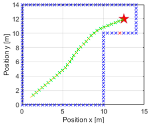
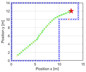
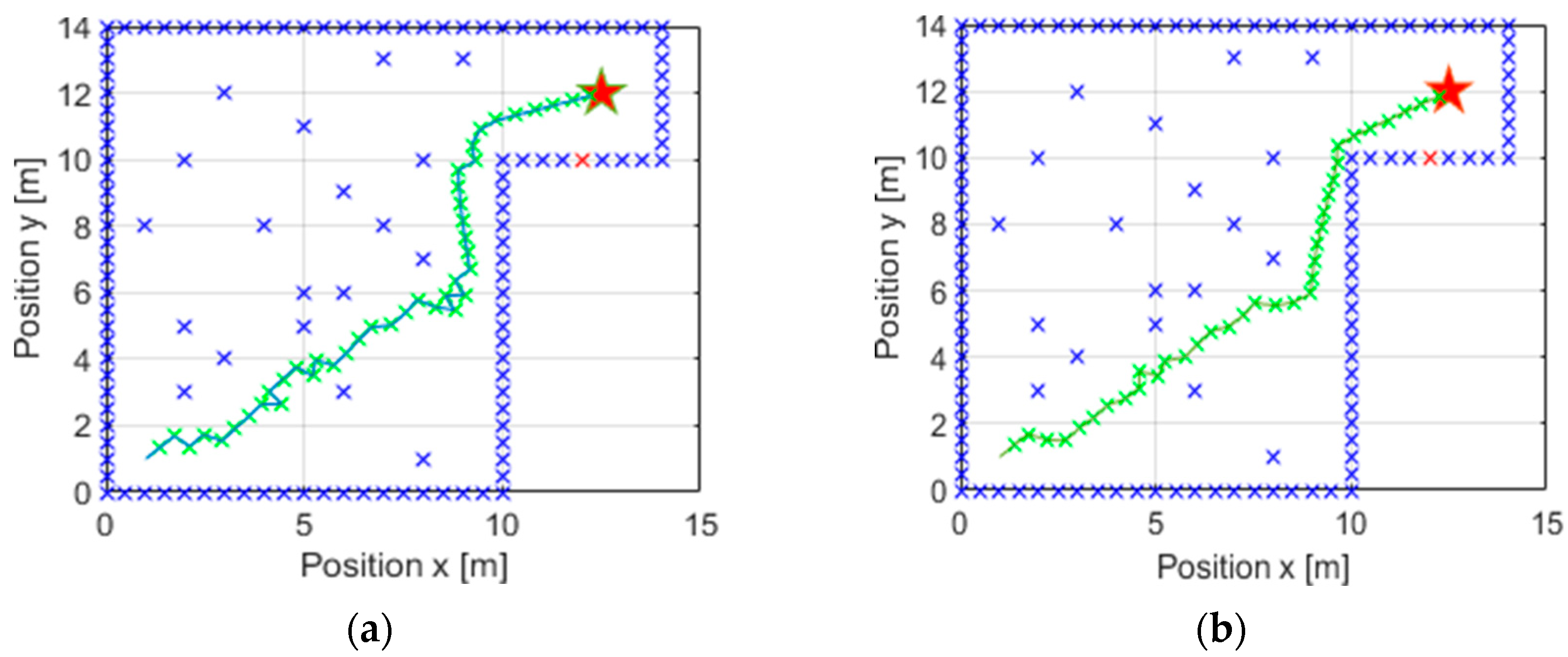
3.3. Variation in the Search Range of the Genetic Algorithm for the Parameter K

As the previous section has shown, there are cases of navigation in which abrupt trajectories are generated, and it is possible that, due to the physical characteristics of the robot, these may not be feasible on many occasions. This happens because in some cases, it is not possible to generalise the range in which the genetic algorithm can search for the $K$ parameter. Therefore, this range, which until now has been fixed between $0.01$ and $1$, has to be varied depending on the case in search of the most optimal navigation.

The case in which the generated trajectory is more abrupt is considered again, that is, the case of the third test performed. It has been observed that the previous parameter K was very large in comparison with the rest, so the decision was taken to limit the search range of the genetic algorithm to values between $0.01$ and $0.1$. This results in an optimal $K$ value of $K=0.0859$, more in line with the rest of the values in Table 5. The following image shows a comparison between the test in the previous section (see Table 4) in which the value of $K$ is not appropriate (Figure 10a) and the navigation carried out with this second more appropriate $K$ parameter (Figure 10b).

As can be appreciated here, by varying the search range of the parameter in the genetic algorithm, navigation is smoother and more feasible in comparison to the previous case, and therefore, it is now more optimal. It is worth mentioning that in this case, the distance travelled is $12.5$ m compared to the $16.5$ m obtained in Figure 10a, and the total reward received is $Q=5845.44$.

Another case is presented here: test 2, seen in Table 4, which generated peaks in the navigation despite being able to continue along a straight trajectory. In this case, it can be noted that the value of $K$ obtained was $K=0.0814$, which is similar to the other values shown in Table 5. However, the navigation was not optimal, so we decided to further limit the search range of the GA. As in the previous case, it was set between $0.01$ and $0.1$, thus obtaining a new $K$ value of $K=0.0331$. Both trajectories can be seen in Figure 11a,b for comparison.

Once again, it can be observed that by limiting the search range of the GA for the value of $K$, a smaller value is achieved, but one that generates more optimal navigation, thus complying with the established requirements. In this case, it should be remembered that the distance travelled in the case of Figure 11a was $12.5$ m (see Table 5), whereas now this distance is reduced by only $0.5$ m. However, navigation is smoother and more achievable, with a cumulative reward of $Q=4000.92$.

In addition, Table 4 shows that the first test also generated more abrupt and less adequate navigation. In this test, a value of $K=0.3862$ was calculated, which was high and did not generate an adequate navigation trajectory, as can be seen in Figure 12a. It should be considered that this is the case where more distance has to be travelled. This means that the vehicle will have to avoid more obstacles and will generate more complicated navigation. This being so, it was necessary to be more restrictive in the search margin given to the genetic algorithm, reducing it to between $0.1$ and $0.6$. In this way, a value of $K=0.10250$ was obtained, more in line with the other tests (see Table 5), and the navigation can be seen in Figure 12b.

In this case, the cumulative reward is $Q=7008.47$ and a distance of $18$ m is covered compared to the $21$ m covered with the higher $K$ value. We consider that the trajectory is not quite optimal, but it improved significantly compared to the previous case, and it is now achievable.

Therefore, it can be argued that it is possible to generate navigation with fixed parameters in the search range of the GA, but sometimes, due to the characteristics of the environment, the generated navigation may not be adequate. Thus, it is shown that with a slight change, it is possible to achieve the desired optimal trajectories without harming either the computational cost or the objectives of the navigation algorithm.

4. Discussion and Conclusions

The proposed evolutionary alternative, that is, the system that performs the adjustment of parameter $K,$ achieved a satisfactory navigation. This optimisation had a direct effect on the action, which was calculated analytically instead of through neural networks, as was done in different studies that attempted to optimise the structure of the network, the reward function and the parameters [43]. In this way, a robust and efficient system has been achieved. It arrives smoothly at the destination from an initial point, accomplishing the navigation goal of an autonomous vehicle.

A previous study was carried out that analysed the stability of DDPG (deep deterministic policy gradient) systems [44], and it was observed that the agents generated with this technique were not capable of generating optimal or complete navigation on many occasions. This research has been continued with the idea of the reward proposed in that study, but how it is derived has been changed, as this time it was conducted analytically, reducing the computational cost. In addition, this method ensures that the target is always reached without colliding with objects. Thus, we concluded to replace the DDPG technique with a combination of reinforcement learning and genetic algorithms.

As far as the reward optimisation system is concerned, it is still a problem to achieve appropriate results [5]. There are also different works that generate a reward gain influenced by vehicle direction and deviation error, in addition to obstacles [2,14], so this approach seems to be appropriate, as they are works that show that arrival at the target was achieved.

Different approaches have been chosen to combine RL with evolutionary techniques. They have attempted to optimise the neural network as if there were only one chromosome in the initial population. Considering the paths as chromosomes and analysing the stretches they perform, it can be seen that the most optimal navigations were not achieved, and if they were, it was necessary to add a technique, such as fuzzy logic [20,45]. Studies have also been carried out paying attention to the topology of the networks and taking their nodes as chromosomes to optimise and try to obtain the best path [46], but it has become a more complex problem.

This paper has presented a navigation algorithm for autonomous guided vehicles that is based on the reward system of reinforcement learning. Only the idea of rewards of the RL algorithm is used, which is the tool to evaluate the controller, but the proposed controller is much simpler, achieving a lower computational cost. For the correct performance of the controller, a parameter K is created, which is optimised through the genetic algorithm technique. This parameter scales the level of the action to be adopted to calculate the navigation instructions. In this way, it is possible to solve the navigation problem. The method achieves the goal of reaching the endpoint and avoiding obstacles along the way, so it can be concluded that it is an efficient and accurate system.

It has been observed that sometimes the trajectories do not satisfy the concept of optimised navigation, but nevertheless, the method meets the expected requirements, being a robust system. In case the navigation is not satisfactory, it has been demonstrated that a slight change in the search margin of the genetic algorithm improves the results significantly, achieving smoother and more achievable trajectories. In addition, the algorithm has been tested with different population sizes of GA, comparing different agents and adapting the population size to the problem presented.

The proposed equation for calculating the action contemplates the relative position of the vehicle at all times and can consider the application of the algorithm in different navigation environments without the need to vary the method, making it a flexible system for any environment. The variation would only consist of the parameter K, as it will vary depending on the complexity of the environment, as we have seen.

In terms of future lines, the next step to be able to verify the efficiency of the navigation algorithm is to implement it outside the simulation in the AGV prototype for which it was designed. The complexity in this part is in considering the size of the vehicle and the size of the surrounding obstacles, so the algorithm needs prior modifications. It is also possible to incorporate computer vision into the algorithm so that it detects the area over which navigation is to be performed. This would give flexibility to the system, allowing the vehicle to adapt to navigation in any environment without prior information about it. Furthermore, as has been seen, the proposed algorithm does not generate optimal trajectories on different occasions, so a study on improvements could also be performed. Also, the equation that evaluates the action to be taken may not consider all possible situations, so it will be necessary to study whether it is adequate in different scenarios.