A New Varying-Factor Finite-Time Recurrent Neural Network to Solve the Time-Varying Sylvester Equation Online

Abstract

This paper presents a varying-parameter finite-time recurrent neural network, called a varying-factor finite-time recurrent neural network (VFFTRNN), which is able to solve the solution of the time-varying Sylvester equation online. The proposed neural network makes the matrix coefficients vary with time and can achieve convergence in a finite time. Apart from this, the performance of the network is better than traditional networks in terms of robustness. It is theoretically proved that the proposed neural network has super-exponential convergence performance. Simulation results demonstrate that this neural network has faster convergence speed and better robustness than the return to zero neural networks and can track the theoretical solution of the time-varying Sylvester equation effectively.

1. Introduction

As we all know, the Sylvester equation $UP-PV+W=0$, as a kind of linear matrix equation, plays a crucial role in many fields, especially linear algebra and matrix theory. For some mathematics, dynamic control systems, and computer vision problems, the Sylvester equation can be used as a solution, like designing a feedback control system by pole assignment optimization, linear least-squares regression, image fusion [1], clustering [2,3], and so on. In recent years, many methods have been proposed by other scholars to solve real-time linear algebra problems [4,5,6,7,8,9,10,11,12,13,14,15,16,17,18]. Among these methods, several are efficient and representative, like gradient-based neural network (GNN) methods and zeroing neural network (ZNN) methods. It is notable that GNN and ZNN methods both use the idea to force the time derivative of the error function decline and further to force the error function gain toward zero. The proposal of GNNs, as emblematic recurrent neural networks, is very representational for solving real-time linear algebra problems [19,20,21]. Generally speaking, different GNNs are designed to solve different linear algebra problems. By itself, for solving the Sylvester equation, the GNN method is roughly stated as follows:

(1)

In the first step, the error function is defined as $E=\left|\right|UP-PV+{W\left|\right|}^2/2$. In order to acquire the solution of the Sylvester equation, the error function should converge to zero.

(2)

In the next step, for the purpose of acquiring the minimum point of the error function, GNN methods use a negative gradient descent direction. In addition to this, GNN methods employ a constant scalar-type parameter, which accelerates the convergence rate of the error function to solve the Sylvester equation efficiently.

However, when the task is time-varying, the traditional GNN method, which is based on gradient-based optimization, has difficulty tracking the ideal solution of the time-varying Sylvester equation. This is because the error, as defined by $E={\displaystyle \frac{\left|\right|UP-PV+{W\left|\right|}^2}{2}}$, cannot converge to zero in such cases, resulting in residual errors [22]. Therefore, a GNN cannot solve the time-varying Sylvester function effectively. But in practice, time-varying problems are everywhere, so we need a neural network to better track locus solutions to time-varying issues in real-time. Under this background, many kinds of neural networks have been proposed to solve this kind of time-varying algebraic problem. Among these neural networks, the ZNN proposed by Zhang et al. proved to be efficient [12]. The ZNN is a kind of implicit dynamic neural network that skillfully replaces the gradient dynamic with an implicit dynamic, so that the computation error can achieve better convergence; that is, with the increase in time, the solution of the network can approach the theoretical solution in real time [23,24,25,26,27,28,29,30,31]. However, the ZNN also has some shortcomings, such as its convergence speed not being fast enough, convergence parameters being difficult to set, and other issues. Aiming to address the above shortcomings, Li et al. proposed a finite-time ZNN [23]. The sign-bi-power activation function is used in this network, as it effectively activates this network, makes the convergence speed much faster, and can achieve finite-time convergence. In addition, Zhang et al. proposed a variable-parameter convergence differential neural network (VP-CDNN) [32]. Different from the initial ZNN, the convergence parameter of the VP-CDNN changes with time, which makes the network hardware implementation much more reasonable than the ZNN, and the convergence speed reaches the super-exponential convergence speed. But despite this, the VP-CDNN cannot achieve finite-time convergence. Based on the above discussion, this paper proposes a recurrent neural network (VFFTRNN) for solving the time-varying Sylvester equation. The network not only has the speed of super-exponential convergence but also can achieve finite-time convergence.

The rest of this paper is divided into four parts. The second section introduces some tools needed to solve the Sylvester equation, and briefly describes the solution steps of the ZNN. In the third section, the implicit dynamic equation of the proposed VFFRTNN and the general steps of solving time-varying problems with the network are given, and the convergence and robustness of VFFTRNN under different conditions are analyzed theoretically. In the fourth section, the simulation results of MATLAB are given and compared with the simulation results of the ZNN. In the last section, the thesis is summarized.

Before concluding this section, some highlights of the paper are listed below:

(1)

We propose a VFFTRNN algorithm for solving the Sylvester equation.

(2)

Compared with VP-CDNN, this network can achieve finite-time convergence.

(3)

We theoretically prove the convergence time of the network in the case of three activation functions.

(4)

In the situation considering the existence of disturbances, the robustness of VFFTRNN is discussed.

(5)

Data simulation results show that the proposed VFFTRNN has better convergence and robustness than the traditional ZNN model under the same initial conditions.

2. Problem Formulation and Knowledge Preparation

Let us observe the following Sylvester equation with smooth time-varying characteristics:

$$\begin{array}{c}\hfill U\left(t\right)P\left(t\right)-P\left(t\right)V\left(t\right)+W\left(t\right)=0,\forall t\in [0,+\infty )\end{array}$$

(1)

where time is expressed as the variable t. The time-varying smooth coefficient matrices are $W\left(t\right)\in {\Re }^{m\times n}$, $V\left(t\right)\in {\Re }^{n\times n}$, as well as $U\left(t\right)\in {\Re }^{m\times m}$. In addition, $\dot{W}\left(t\right)=$ d$W\left(t\right)$/dt, $\dot{V}\left(t\right)=$ d$V\left(t\right)$/dt, and $\dot{U}\left(t\right)=$ d$U\left(t\right)$/dt are their time derivatives, respectively, assuming these time derivatives are known or can be found exactly. Furthermore, $P\left(t\right)\in {\Re }^{m\times n}$ is uncharted but real, and our purpose is to find it to approach or even obtain the unique ideal solution $P^{*}\left(t\right)$ in finite time for the above Sylvester equation.

In order to facilitate the subsequent discussion and to solve Equation (1) more simply, (1) is best to be transformed into a vector form. The following Theorem (1) is introduced.

Theorem 1.

The Sylvester equation in matrix form (i.e., Equation (1)) can be transformed into vector form as follows:

$$\begin{array}{c}\hfill \left(I_n\otimes U\left(t\right)-V^T\left(t\right)\otimes I_m\right)vec\left(P\left(t\right)\right)+vec\left(W\left(t\right)\right)=0\end{array}$$

(2)

where $I_n$ and $I_m$ represent the n-dimensional and m-dimensional identity matrices, respectively. Additionally, the symbol T represents the transpose of the matrix. The symbol $\otimes$ denotes the Kronecker product. In other words, $U\otimes V\in {\Re }^{mn\times mn}$ represents a large matrix, which is equivalent to transforming the $ith$ row and j−column position element $u_{ij}$ in the matrix U into a matrix $u_{ij}V$. The operation $vec\left(P\left(t\right)\right)\in {\Re }^{mn}$ represents a column vector obtained by stacking the columns of the matrix $P\left(t\right)\in {\Re }^{m\times n}$ in sequence.

Proof. 

See Section 2 and [12], Appendix. □

Furthermore, if we want to obtain the unique solution of Equation (1), then it must meet the regularity condition [12,33], which is described in the following Theorem (2).

Theorem 2.

If the Sylvester Equation (1) satisfies the following regularity condition, then it has a unique solution.

$$\begin{array}{c}\hfill I_n\otimes \left(U^T\left(t\right)U\left(t\right)\right)-V^T\left(t\right)\otimes U^T\left(t\right)-V\left(t\right)\otimes U\left(t\right)\\ \hfill +\left(V\left(t\right)V^T\left(t\right)\right)\otimes I_m\ge \alpha I_{mn},\exists \alpha >0,\forall t\in [0,+\infty )\end{array}$$

(3)

where $I_{mn}$ represents the mn-dimensional identity matrix.

Proof. 

See Section 2 and [12], Appendix. □

With the continuous development of neural dynamics and the proposal of ZNNs, the concept of ZNNs has been applied in many engineering and scientific fields to solve time-varying problems. To clarify the details of this paper, we will next briefly introduce how to solve the Sylvester Equation (1) using a typical ZNN method.

In the first step, an error function for Equation (1) is defined as follows:

$$\begin{array}{c}\hfill E\left(t\right):=U\left(t\right)P\left(t\right)-P\left(t\right)V\left(t\right)+W\left(t\right)\end{array}$$

(4)

Next, since our goal is to obtain a unique solution to Equation (1), when we set the error function to approach 0, the unique solution of Equation (1) will be obtained naturally. In light of the design principles of neurodynamics, the following differential equations for the error function $E\left(t\right)$ can be designed:

$$\begin{array}{c}\hfill {\displaystyle \frac{dE\left(t\right)}{dt}}=\dot{E}\left(t\right)=-\mu \Phi \left(E\left(t\right)\right)\end{array}$$

(5)

where the scale-valued factor $\mu$ is a positive design constant (i.e., $\mu >0$), which can adjust the convergence velocity of this network (5) by varying its value. $\Phi (·):{\Re }^{m\times n}\to {\Re }^{m\times n}$ is an array consisting of the same activation functions. $\Phi (·)$ can represent different types of activation functions, such as linear-type, bipolar-sigmoid-type, power-type, sign-bi-power-type, and so on. When we use the activation function of the linear type, (5) becomes a typical ZNN.

Based on (5), we can obtain the following implicit dynamic equation:

$$\begin{array}{c}\hfill U\left(t\right)\dot{P}\left(t\right)-\dot{P}\left(t\right)V\left(t\right)+\dot{U}\left(t\right)P\left(t\right)-P\left(t\right)\dot{V}\left(t\right)\\ \hfill +\dot{W}\left(t\right)=-\mu \Phi \left(U\left(t\right)P\left(t\right)-P\left(t\right)V\left(t\right)+W\left(t\right)\right)\end{array}$$

(6)

where the starting value of $P\left(t\right)$ is $P\left(0\right)=P_0\in R^{m\times n}$. Additionally, the state matrix $P\left(t\right)$ is an approximate solution that will gradually approach the theoretical solution, and it will converge to the unique solution of $\left(1\right)$. In light of the following lemma [12], the performance of the ZNNs in solving the Sylvester equation can be guaranteed to exhibit exponential convergence.

Lemma 1.

Considering the Sylvester Equation (1), with its time-varying coefficient matrices $U\left(t\right)\in {\Re }^{m\times m}$, $V\left(t\right)\in {\Re }^{n\times n}$, and $W\left(t\right)\in {\Re }^{m\times n}$, and assuming that they satisfy inequality (3), if the activation function of the implicit dynamic Equation (6) is chosen to be linear, then its state matrix $P\left(t\right)$ will exponentially converge from any initial state $P_0$ to the time-varying ideal solution $P^{*}\left(t\right)$ of (1).

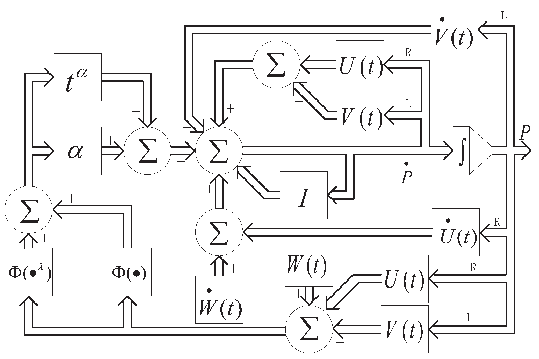
3. Varying-Factor Finite-Time Recurrent Neural Networks

ZNN can achieve better convergence performance by using different activation functions or setting a larger constant factor [34], but its convergence still has room for improvement. Inspired by classic ZNN design principles, a novel recurrent neural network is proposed in this paper. It can achieve a neural network with super-exponential convergence within a limited time, and because the factor before its activation function changes with time, it is called VFFTRNN. It can be expressed as

$$\begin{array}{cc}\hfill \dot{E}\left(t\right)& =-\Gamma \left(t\right)\left(\Phi \left(E\left(t\right)\right)+\Phi \left(E^{\lambda }\left(t\right)\right)\right)\hfill \\ \hfill & =-(t^{\alpha }+\alpha )\left(\Phi \left(E\left(t\right)\right)+\Phi \left(E^{\lambda }\left(t\right)\right)\right)\hfill \end{array}$$

(7)

where $\Gamma \left(t\right)$ is a function of t, and it can be set to different functions. For simplicity, we use exponential time-varying parameters $(t^{\alpha }+\alpha )$, where $\alpha$ is a positive scalar-valued factor (i.e., $\alpha >0$), and the positive scalar-valued factor $\lambda ={\displaystyle \frac{s}{q}}\in (0,1)$, where s and q are odd numbers. In light of (7), we can reformulate its implicit dynamic equation as

$$\begin{array}{cc}\hfill \dot{U}\left(t\right)& P\left(t\right)+U\left(t\right)\dot{P}\left(t\right)-\dot{P}\left(t\right)V\left(t\right)-P\left(t\right)\dot{V}\left(t\right)+\dot{W}\left(t\right)\hfill \\ \hfill =& -(t^{\alpha }+\alpha )(\Phi \left(U\left(t\right)P\left(t\right)-P\left(t\right)V\left(t\right)+W\left(t\right)\right)\hfill \\ \hfill & +\Phi {\left(U\left(t\right)P\left(t\right)-P\left(t\right)V\left(t\right)+W\left(t\right)\right)}^{\lambda })\hfill \end{array}$$

(8)

In addition, in light of Theorem 1 and Equation (2) in Section 1, we are able to obtain the vector form of the above implicit dynamic Equation (8):

$$\begin{array}{cc}\hfill N\left(t\right)\dot{p}\left(t\right)=& -\dot{N}\left(t\right)p\left(t\right)-vec\left(\dot{W}\left(t\right)\right)\hfill \\ \hfill & -(t^{\alpha }+\alpha )(\Phi \left(N\left(t\right)p\left(t\right)+vec\left(W\left(t\right)\right)\right)\hfill \\ \hfill & +\Phi {\left(N\left(t\right)p\left(t\right)+vec\left(W\left(t\right)\right)\right)}^{\lambda })\hfill \end{array}$$

(9)

where $N\left(t\right):=I_n\otimes U\left(t\right)-V^T\left(t\right)\otimes I_m\in {\Re }^{mn\times mn}$ is a matrix, $p\left(t\right):=vec\left(P\left(t\right)\right)\in {\Re }^{mn}$ is a vector, and $\Phi (·):{\Re }^{mn\times 1}\to {\Re }^{mn\times 1}$ is an activation function array. It is noteworthy that the transformation dimensions of $\Phi (·)$ in (9) are different from those in (5). The block diagram of VFFTRNN can be drawn based on the implicit dynamic Equation (8). As shown in Figure 1, ∫ and ∑ represent the integrator and accumulator, respectively. The symbols L and R represent left and right matrix multiplication, respectively.

3.1. Convergence Analysis

The following theorem will lay the foundation for later reference when discussing the global convergence of VFFTRNN.

Theorem 3.

For the time-varying Sylvester Equation (1), its coefficient matrices $U\left(t\right)\in {\Re }^{m\times m}$, $V\left(t\right)\in {\Re }^{n\times n}$, and $W\left(t\right)\in {\Re }^{m\times n}$ are given. If Equation (1) satisfies inequality (3), and the activation function sequence is chosen to be strictly increasing, then the state matrix $P\left(t\right)$ of the VFFTRNN model (8) will globally converge from any initial state $P_0$ to the time-varying ideal solution $P^{*}\left(t\right)$ of the Sylvester Equation (1).

Proof. 

First, we can convert the VFFTRNN system (7) into scalar form as follows:

$$\begin{array}{c}\hfill {\dot{e}}_{ij}\left(t\right)=-(t^{\alpha }+\alpha )\left(\varphi \left(e_{ij}\left(t\right)\right)+\varphi \left(e_{ij}^{\lambda }\left(t\right)\right)\right)\\ \hfill \forall i\in \{1,2,\dots m\},j\in \{1,2,\dots n\}\end{array}$$

(10)

where $e_{ij}\left(t\right)$ represents the $ith$ row and j− column position element of $E\left(t\right)$. In addition, $\varphi (·)$ represents the activation subfunction for the matrix elements.

Next, we will prove its global convergence. Let us define a Lyapunov function as shown below:

$$v_{ij}\left(t\right)={\displaystyle \frac{1}{2}}{e}_{ij}^2\left(t\right),\forall i\in \{1,2,\dots m\},j\in \{1,2,\dots n\}$$

(11)

According to the above, we can calculate its time derivative as follows:

$$\begin{array}{cc}\hfill {\dot{v}}_{ij}\left(t\right)& =e_{ij}\left(t\right){\dot{e}}_{ij}\left(t\right)\hfill \\ \hfill & =-(t^{\alpha }+\alpha )e_{ij}\left(\varphi \left(e_{ij}\left(t\right)\right)+\varphi \left(e_{ij}^{\lambda }\left(t\right)\right)\right)\hfill \end{array}$$

It can be seen from the previous definition that $\alpha >0$ and $\varphi (·)$ is monotonic and strictly increasing. Thus, for any $t\ge 0$ and $e_{ij}\left(t\right)$, we have

$$\begin{array}{c}\hfill {\dot{v}}_{ij}\left(t\right)\left\{\begin{array}{c}=0e_{ij}\left(t\right)=0\hfill \\ \le 0e_{ij}\left(t\right)\ne 0.\hfill \end{array}\right.\end{array}$$

In light of Lyapunov stability theory, the error function (10) is globally asymptotically convergent. Therefore, for any i and j in the domain, the error function $e_{ij}\left(t\right)$ in scalar form will asymptotically converge to zero. In other words, the online solution $P\left(t\right)$ using VFFTRNN will approach its theoretical solution $P^{*}\left(t\right)$ when $t\to +\infty$.

In conclusion, the proof of Theorem 3 has been completed. That is, VFFTRNN exhibits global asymptotic convergence. □

In the next step, we will demonstrate the finite-time convergence of VFFTRNN under various activation functions (i.e., linear, bipolar-sigmoid, and power functions). See the following theorem for the specific convergence time.

Theorem 4.

For the time-varying Sylvester Equation (1), the coefficient matrices $U\left(t\right)\in {\Re }^{m\times m}$, $V\left(t\right)\in {\Re }^{n\times n}$ and $W\left(t\right)\in {\Re }^{m\times n}$ have been given. If Equation (1) satisfies the regularity condition (3) and the activation function sequence is monotonic and strictly increasing, then the VFFTRNN system (8) can converge to the theoretical solution $P^{*}\left(t\right)$ of Equation (1) in finite time from any arbitrary initial state. In addition, the specific convergence time of the neural system $\left(7\right)$ in the cases of different activation functions is as follows:

(1) 

When we choose the linear activation function (i.e., $\varphi \left(x\right)=x$), the convergence time of VFFTRNN $t_c<t_L$.

(2) 

When we choose the bipolar-sigmoid activation function (i.e., $\varphi \left(x\right)=(1-exp(-\xi x\left)\right)/(1+exp(-\xi x\left)\right)$, $\xi >0$), the convergence time of VFFTRNN $t_c<t_B$.

(3) 

When we choose the power activation function (i.e., $\varphi \left(x\right)=x^s$, $\lambda s<1$ and s is an odd number), the convergence time of VFFTRNN $t_c<t_P$.

The above $t_L$, $t_B$ and $t_P$ are, respectively,

$$\begin{array}{cc}\hfill & t_L=\sqrt[\alpha +1]{{\displaystyle \frac{\alpha +1}{1-\lambda }}ln({\chi }_1^{1-\lambda }+1)}\hfill \\ \hfill & t_B=\left\{\begin{array}{cc}\sqrt[\alpha +1]{{\displaystyle \frac{\alpha +1}{\omega (1-\lambda )}}ln({\chi }_1^{1-\lambda }+1)}\hfill & if {\chi }_1\le 1\hfill \\ \sqrt[\alpha +1]{{\displaystyle \frac{\alpha +1}{\omega (1-\lambda )}}ln\left(2\right)+{\displaystyle \frac{(\alpha +1)({\chi }_1-1)}{\omega }}}\hfill & otherwise.\hfill \end{array}\right.\hfill \\ & t_P=\left\{\begin{array}{cc}\sqrt[\alpha +1]{{\displaystyle \frac{\alpha +1}{2(1-\lambda s)}}{\chi }_1^{1-\lambda s}}\hfill & if {\chi }_1\le 1\hfill \\ \sqrt[\alpha +1]{{\displaystyle \frac{\alpha +1}{2(1-\lambda s)}}+{\displaystyle \frac{(\alpha +1)({\chi }_1^{1-s}-1)}{2(1-s)}}}\hfill & otherwise.\hfill \end{array}\right.\hfill \end{array}$$

where ${\chi }_1$ represents $max\left(\right|e_{ij}\left(0\right)\left|\right)$.

Proof. 

In the following, we will prove the convergence time of the VFFTRNN system under three different activation functions, one by one.

(1)

Linear-type: For the linear-type case, the following equation can be obtained from (10).

$${\dot{e}}_{ij}\left(t\right)=-(t^{\alpha }+\alpha )\left(e_{ij}\left(t\right)+e_{ij}^{\lambda }\left(t\right)\right)$$

(12)

In light of differential equation theory [34], we can obtain the solution of (12).

$$e_{ij}\left(t\right)={\left((e_0^{1-\lambda }+1)exp\left((\lambda -1)(\alpha t+{\displaystyle \frac{t^{\alpha +1}}{\alpha +1}})\right)-1\right)}^{{\displaystyle \frac{1}{1-\lambda }}}$$

(13)

where $e_0=e_{ij}\left(0\right)$. Let $e_{ij}\left(t\right)$ in (13) be equal to zero, and we can obtain the following:

$$\begin{array}{c}\hfill \alpha t+{\displaystyle \frac{t^{\alpha +1}}{\alpha +1}}={\displaystyle \frac{ln(e_0^{1-\lambda }+1)}{1-\lambda }}\ge {\displaystyle \frac{t^{\alpha +1}}{\alpha +1}}\end{array}$$

then we can easily find $t\le \sqrt[\alpha +1]{{\displaystyle \frac{\alpha +1}{1-\lambda }}ln(e_0^{1-\lambda }+1)}$. In other words, for any i and j in the definitional domain, we have that as $t\to \sqrt[\alpha +1]{{\displaystyle \frac{\alpha +1}{1-\lambda }}ln(e_0^{1-\lambda }+1)}$, the scalar value $e_{ij}\left(t\right)\to 0$. Note that by the definition of $e_{ij}\left(t\right)$ above, at this time, the error function $E\left(t\right)$ in matrix form will also approach zero, which guarantees that the state matrix $P\left(t\right)\to P^{*}\left(t\right)$.

To sum up, we can obtain the convergence time when the VFFTRNN system uses the linear-type function as follows:

$$t_L=\sqrt[\alpha +1]{{\displaystyle \frac{\alpha +1}{1-\lambda }}ln({\chi }_1^{1-\lambda }+1)}$$

(14)

where ${\chi }_1=max\left(\right|e_{ij}\left(0\right)\left|\right)$. This shows that in the case where the activation function is linear, the VFFTRNN method can achieve finite-time convergence in solving the Sylvester equation.

(2)

Bipolar-Sigmoid-Type: In this case, we can easily see that the activation function is $\varphi \left(x\right)=(1-exp(-\xi x\left)\right)/(1+exp(-\xi x\left)\right)$, where $\varphi \ge 1$ and $x\in R$ are scalar factors. The following equation can be obtained from (10).

$$\begin{array}{c}{\dot{e}}_{ij}\left(t\right)=-(t^{\alpha }+\alpha )\left(R\right(t)+Q(t\left)\right)=\hfill \\ -(t^{\alpha }+\alpha )(\frac{1-\exp (-\xi e_{ij}\left(t\right))}{1+\exp (-\xi e_{ij}\left(t\right))}+\frac{1-\exp (-\xi e_{ij}^{\lambda }\left(t\right))}{1+\exp (-\xi e_{ij}^{\lambda }\left(t\right))})\hfill \end{array}$$

(15)

where $R\left(e_{ij}\left(t\right)\right)={\displaystyle \frac{1-\exp (-\xi e_{ij}\left(t\right))}{1+\exp (-\xi e_{ij}\left(t\right))}}$, $Q\left(e_{ij}\left(t\right)\right)={\displaystyle \frac{1-\exp (-\xi e_{ij}^{\lambda }\left(t\right))}{1+\exp (-\xi e_{ij}^{\lambda }\left(t\right))}}$. In light of the relevant theory of differential equations, we can rewrite (15) as follows:

$$\begin{array}{c}\hfill {\displaystyle \frac{dy}{dt}}=-(t^{\alpha }+\alpha )\left(R\left(y\right)+Q\left(y\right)\right)\end{array}$$

where $y=e_{ij}\left(t\right)$. According to the Lyapunov function of this system, we know that $e_{ij}\left(t\right)$ either increases or decreases monotonically as t increases. For simplicity, we will next discuss the case where $e_{ij}\left(0\right)=y_0\ge 0$. In this case, we can derive the following:

$${\int }_0^t(t^{\alpha }+\alpha )dt=-{\int }_{y_0}^0{\displaystyle \frac{1}{R\left(y\right)+Q\left(y\right)}}dy$$

(16)

At this point, we consider the following two situations.

a.

When $y_0\le 1$, noticing that $R\left(y\right)$ and $Q\left(y\right)$ are convex, solving (16) gives

$$\begin{array}{cc}\hfill \alpha t+\frac{t^{\alpha +1}}{\alpha +1}& ={\int }_0^{y_0}\frac{1}{R\left(y\right)+Q\left(y\right)}dy\hfill \\ \hfill & \le {\displaystyle \frac{1}{\omega }}{\int }_0^{y_0}{\displaystyle \frac{1}{y+y^{\lambda }}}dy\hfill \\ \hfill & =\frac{1}{\omega (1-\lambda )}ln(y_0^{1-\lambda }+1)\hfill \end{array}$$

(17)

where $\omega =R\left(1\right)=Q\left(1\right)=(1-exp(-\xi \left)\right)/(1+exp(-\xi \left)\right)$ is a constant, determined by the scalar factor $\xi$. Similar to linear-type, solving for (17), we obtain

$$t\le \sqrt[\alpha +1]{{\displaystyle \frac{\alpha +1}{\omega (1-\lambda )}}ln(y_0^{1-\lambda }+1)}$$

(18)

b.

When $y_0>1$, based on Equations (16) and (17), Equation (19) be derived:

$$\begin{array}{cc}\hfill & \alpha t+{\displaystyle \frac{t^{\alpha +1}}{\alpha +1}}\hfill \\ \hfill & ={\int }_0^1{\displaystyle \frac{1}{R\left(y\right)+Q\left(y\right)}}dy+{\int }_1^{y_0}{\displaystyle \frac{1}{R\left(y\right)+Q\left(y\right)}}dy\hfill \\ \hfill & \le {\displaystyle \frac{1}{\omega (1-\lambda )}}ln2+{\int }_1^{y_0}{\displaystyle \frac{1}{R\left(y\right)+Q\left(y\right)}}dy\hfill \end{array}$$

(19)

Notice that $R\left(y\right)$ and $Q\left(y\right)$ are monotonically increasing over the interval $y>0$, so for $y>1$, $R\left(y\right)>R\left(1\right)>\omega$ and $Q\left(y\right)>Q\left(1\right)>\omega$. Therefore, we have

$$\begin{array}{c}\hfill {\int }_1^{y_0}{\displaystyle \frac{1}{R\left(y\right)+Q\left(y\right)}}dy\le {\int }_1^{y_0}{\displaystyle \frac{1}{\omega }}dy={\displaystyle \frac{y_0-1}{\omega }}\end{array}$$

(20)

Substituting (20) into (19) and solving, we obtain

$$t\le \sqrt[\alpha +1]{{\displaystyle \frac{\alpha +1}{\omega (1-\lambda )}}ln2+{\displaystyle \frac{(\alpha +1)(y_0-1)}{\omega }}}$$

(21)

In light of the results (18) and (21) from the two situations, it can be concluded that when $t\to \sqrt[\alpha +1]{{\displaystyle \frac{\alpha +1}{\omega (1-\lambda )}}ln(y_0^{1-\lambda }+1)}$ or $t\to \sqrt[\alpha +1]{{\displaystyle \frac{\alpha +1}{\omega (1-\lambda )}}ln2+{\displaystyle \frac{(\alpha +1)(y_0-1)}{\omega }}}$, the scalar value $e_{ij}\left(t\right)\to 0$ for any i and j in the defined domain. This means that the convergence of the state matrix $P\left(t\right)\to P^{*}\left(t\right)$ is guaranteed. Thus, the convergence time for the bipolar-sigmoid-type activation function can be expressed as

$$\begin{array}{cc}\hfill t& <\left\{\begin{array}{cc}\sqrt[\alpha +1]{{\displaystyle \frac{\alpha +1}{\omega (1-\lambda )}}ln({\chi }_1^{1-\lambda }+1)}\hfill & \mathrm{if} {\chi }_1\le 1\hfill \\ \sqrt[\alpha +1]{{\displaystyle \frac{\alpha +1}{\omega (1-\lambda )}}ln2+{\displaystyle \frac{(\alpha +1)({\chi }_1-1)}{\omega }}}\hfill & \mathrm{if} \mathrm{otherwise}.\hfill \end{array}\right.\hfill \\ & =t_B\hfill \end{array}$$

(22)

(3)

Power-Type: For the power-type case, the activation function is defined as $\varphi \left(x\right)=x^s$, where s is an odd number and $\lambda s<1$. In this case, the following equation can be derived from (10).

$${\dot{e}}_{ij}\left(t\right)=-(t^{\alpha }+\alpha )\left(e_{ij}^s\left(t\right)+e_{ij}^{\lambda s}\left(t\right)\right)$$

(23)

• Similar to (16), we have

  $${\displaystyle \frac{t^{\alpha +1}}{\alpha +1}}+\alpha t={\int }_0^{y_0}{\displaystyle \frac{1}{y^s+y^{\lambda s}}}dy$$

  (24)
• The discussion is divided into the following two situations:

a.

When $y_0\le 1$, it can be found that $1>\lambda s>s$, so $y^s>y^{\lambda s}$. In light of (24), we can obtain

$$\begin{array}{c}\hfill {\displaystyle \frac{t^{\alpha +1}}{\alpha +1}}+\alpha t\le {\int }_0^{y_0}{\displaystyle \frac{1}{2y^{\lambda s}}}dy={\displaystyle \frac{1}{2(1-\lambda s)}}{y}_0^{1-\lambda s}\end{array}$$

Then, the result (25) can be obtained:

$$t<\sqrt[\alpha +1]{{\displaystyle \frac{\alpha +1}{2(1-\lambda s)}}{y}_0^{1-\lambda s}}$$

(25)

b.

When $y_0>1$, we know that for all $y>1$, we have $y^p<y^{\lambda s}$. So similarly,

$$\begin{array}{cc}\hfill {\displaystyle \frac{t^{\alpha +1}}{\alpha +1}}+\alpha t& \le {\int }_0^1{\displaystyle \frac{1}{2y^{\lambda s}}}dy+{\int }_1^{y_0}{\displaystyle \frac{1}{2y^s}}dy\hfill \\ \hfill & ={\displaystyle \frac{1}{2(1-\lambda s)}}+{\displaystyle \frac{y_0^{1-s}-1}{2(1-s)}}\hfill \end{array}$$

Then, the following result (26) can be obtained:

$$t<\sqrt[\alpha +1]{{\displaystyle \frac{\alpha +1}{2(1-\lambda s)}}+{\displaystyle \frac{(\alpha +1)(y_0^{1-s}-1)}{2(1-s)}}}$$

(26)

In conclusion, when $t\to \sqrt[\alpha +1]{{\displaystyle \frac{\alpha +1}{2(1-\lambda s)}}{y}_0^{1-\lambda s}}$ or $t\to \sqrt[\alpha +1]{{\displaystyle \frac{\alpha +1}{2(1-\lambda s)}}+{\displaystyle \frac{(\alpha +1)(y_0^{1-s}-1)}{2(1-s)}}}$, the scalar value $e_{(ij}\left(t\right)\to 0$ for any i and j on the definitional domain. This means that the convergence of state matrix $P\left(t\right)\to P^{*}\left(t\right)$ is guaranteed. The convergence time for the power-type activation function can be represented as

$$\begin{array}{cc}\hfill t& <\left\{\begin{array}{cc}\sqrt[\alpha +1]{{\displaystyle \frac{\alpha +1}{2(1-\lambda s)}}{\chi }_1^{1-\lambda s}}\hfill & \mathrm{if} {\chi }_1\le 1\hfill \\ \sqrt[\alpha +1]{{\displaystyle \frac{\alpha +1}{2(1-\lambda s)}}+{\displaystyle \frac{(\alpha +1)({\chi }_1^{1-s}-1)}{2(1-s)}}}\hfill & \mathrm{if} \mathrm{otherwise}.\hfill \end{array}\right.\hfill \\ & =t_P\hfill \end{array}$$

(27)

In light of the above analysis, it can be concluded that VFFTRNN achieves finite-time convergence in solving the Sylvester Equation (1), regardless of the choice of activation function. Therefore, the proof of Theorem 4 on finite-time convergence is completed. □

Remark 1.

Regardless of the chosen activation function, the convergence time of VFFTRNN is determined by the initial error $E\left(0\right)$ (i.e., $E\left(0\right)=U\left(0\right)P\left(0\right)+P\left(0\right)V\left(0\right)-W\left(0\right)$) and the design factors $\alpha$ and $\lambda$.

Next, we will analyze the influence of the factors $\alpha$ and $\lambda$ on the convergence time for different activation functions.

(1)

Linear-Type:

a.

For $\alpha$, in light of (14), $t_L$ can be rewritten as

$$t_L={\left({\chi }_2{\alpha }_1\right)}^{{\displaystyle \frac{1}{{\alpha }_1}}}$$

(28)

where ${\chi }_2={\displaystyle \frac{\ln ({\chi }_1^{1-\lambda }+1)}{1-\lambda }}>0$ and ${\alpha }_1=\alpha +1>1$. Then, let us take the partial derivative with respect to ${\alpha }_1$.

$${\displaystyle \frac{\partial t_L}{\partial {\alpha }_1}}={\left({\chi }_2{\alpha }_1\right)}^{{\displaystyle \frac{1}{{\alpha }_1}}}{\displaystyle \frac{1-\ln \left({\chi }_2{\alpha }_1\right)}{{\alpha }_1^2}}$$

(29)

We know that if ${\alpha }_1$ is large enough, $1-ln\left({\chi }_2{\alpha }_1\right)$ will become less than zero. Therefore, for ${\displaystyle \frac{\partial t_L}{\partial {\alpha }_1}}$, there are two possible situations:

$$\begin{array}{c}\hfill \left\{\begin{array}{c}{\displaystyle \frac{\partial t_L}{\partial {\alpha }_1}}<0\forall {\alpha }_1>1\hfill \\ {\displaystyle \frac{\partial t_L}{\partial {\alpha }_1}}>0\exists {\alpha }_1>1\hfill \end{array}\right.\end{array}$$

In the first situation, $t_L$ decreases as ${\alpha }_1$ increases. In other words, as $\alpha$ increases, $t_L$ decreases simultaneously. Similarly, in the second situation, $t_L$ will first increase and then decrease as $\alpha$ increases. This means that when $\alpha$ reaches a specific value, determined by the initial error $E\left(0\right)$, $t_L$ will attain its maximum.

b.

For $\lambda$, in light of (14), it can easily be seen that we only need to analyze ${\displaystyle \frac{\ln ({\chi }_1^{1-\lambda }+1)}{1-\lambda }}$. Next, take the partial derivative of this expression:

$${\displaystyle \frac{\partial \eta }{\partial {\lambda }_1}}={\displaystyle \frac{{\lambda }_1{\chi }_1^{{\lambda }_1}\ln {\chi }_1-({\chi }_1^{{\lambda }_1}+1)\ln ({\chi }_1^{{\lambda }_1}+1)}{{\lambda }_1^2}}$$

(30)

where $\eta ={\displaystyle \frac{\ln ({\chi }_1^{1-\lambda }+1)}{1-\lambda }}$ and ${\lambda }_1=1-\lambda \in (0,1)$. Since the denominator of (30) is always positive, we only need to analyze the numerator:

$${\lambda }_1{\chi }_1^{{\lambda }_1}\ln {\chi }_1-({\chi }_1^{{\lambda }_1}+1)\ln ({\chi }_1^{{\lambda }_1}+1)$$

(31)

If ${\chi }_1\le 1$, then ${\lambda }_1{\chi }_1^{{\lambda }_1}\ln {\chi }_1\le 0$, and ${\lambda }_1{\chi }_1^{{\lambda }_1}\ln {\chi }_1-({\chi }_1^{{\lambda }_1}+1)\ln ({\chi }_1^{{\lambda }_1}+1)<0$. Therefore, the value of (30) is always less than zero. If ${\chi }_1>1$, let ${\chi }_1^{{\lambda }_1}={\lambda }_2>1$, then ${\lambda }_1={\displaystyle \frac{\ln {\lambda }_2}{\ln {\chi }_1}}$. The numerator can be rewritten as follows:

$$\begin{array}{cc}\hfill & {\lambda }_1{\chi }_1^{{\lambda }_1}\ln {\chi }_1-({\chi }_1^{{\lambda }_1}+1)\ln ({\chi }_1^{{\lambda }_1}+1)\hfill \\ \hfill & ={\lambda }_2\ln {\lambda }_2-({\lambda }_2+1)\ln ({\lambda }_2+1)\hfill \end{array}$$

(32)

Note that the function $f\left(x\right)=x\ln x$ is monotonically increasing when $x>1$. Therefore, the value of Equation (32) is always less than zero. In other words, the value of Equation (30) is always less than zero.

Based on the above discussion, we can conclude that for any ${\lambda }_1$, it is always true that ${\displaystyle \frac{\partial \eta }{\partial {\lambda }_1}}<0$. Considering the relationship between ${\lambda }_1$ and $\lambda$, we can conclude that when $\lambda$ is larger, $t_L$ is smaller.

(2)

Bipolar-Sigmoid-Type:

a.

For $\alpha$, in light of (22), $t_B$ can be rewritten as

$$\begin{array}{c}\hfill t_B={\left({\chi }_3{\alpha }_1\right)}^{{\displaystyle \frac{1}{{\alpha }_1}}}\end{array}$$

(33)

where ${\chi }_3=\left\{\begin{array}{c}{\displaystyle \frac{\ln ({\chi }_1^{1-\lambda }+1)}{\omega (1-\lambda )}}>0,{\chi }_1\le 1\hfill \\ {\displaystyle \frac{\ln 2}{\omega (1-\lambda )}}+{\displaystyle \frac{{\chi }_1-1}{\omega }}>0,{\chi }_1>1\hfill \end{array}\right.$. Similar to the analysis of the linear-type above, there are two situations:

$$\begin{array}{c}\hfill \left\{\begin{array}{c}{\displaystyle \frac{\partial t_B}{\partial {\alpha }_1}}<0\forall {\alpha }_1>1\hfill \\ {\displaystyle \frac{\partial t_B}{\partial {\alpha }_1}}>0\exists {\alpha }_1>1\hfill \end{array}\right.\end{array}$$

For the first situation, when $\alpha$ increases, $t_B$ decreases. For the second situation, there exists a specific value where $t_B$ is maximized.

b.

For $\lambda$, by analyzing the structure of Equation (22), we focus on ${\displaystyle \frac{\ln ({\chi }_1^{1-\lambda }+1)}{1-\lambda }}$ when ${\chi }_1\le 1$ and ${\displaystyle \frac{\ln 2}{1-\lambda }}$ when ${\chi }_1>1$. As $\lambda$ increases, the value of ${\displaystyle \frac{\ln 2}{1-\lambda }}$ increases, Based on the derivation in Section 1), it is evident that for any $\lambda \in (0,1)$, as $\lambda$ increases, $t_B$ also increases.

In addition, consider the influence of the factor $\xi$ on the convergence time $t_B$. We know that $\omega ={\displaystyle \frac{1-e^{-\xi }}{1+e^{-\xi }}}$, and as $\xi$ increases, $\omega$ also increases. Furthermore, according to Equation (22), the larger $\omega$ is, the smaller $t_B$ becomes.

(3)

Power-Type:

a.

For $\alpha$, let ${\chi }_4=\left\{\begin{array}{c}{\displaystyle \frac{{\chi }_1^{1-\lambda s}}{2(1-\lambda s)}}>0,{\chi }_1\le 1\hfill \\ {\displaystyle \frac{1}{2(1-\lambda s)}}+{\displaystyle \frac{1-{\chi }_1^{s-1}}{2(s-1)}}>0,{\chi }_1>1\hfill \end{array}\right.$, then we have

$$t_P={\left({\chi }_4{\alpha }_1\right)}^{{\displaystyle \frac{1}{{\alpha }_1}}}$$

(34)

Similar to the analysis of the linear-type case above, there are two possible situations:

$$\begin{array}{c}\hfill \left\{\begin{array}{c}{\displaystyle \frac{\partial t_P}{\partial {\alpha }_1}}<0\forall {\alpha }_1>1\hfill \\ {\displaystyle \frac{\partial t_P}{\partial {\alpha }_1}}>0\exists {\alpha }_1>1\hfill \end{array}\right.\end{array}$$

For the first situation, when $\alpha$ increases, $t_P$ decreases. For the second situation, there exists a certain value where $t_P$ is maximized.

b.

For $\lambda$, according to (27), we can conclude that the larger $\lambda$ is, the larger $t_P$ becomes, especially when ${\chi }_1>0$. In addition, when ${\chi }_1\le 1$, we only need to consider ${\displaystyle \frac{{\chi }^{1-\lambda s}}{1-\lambda s}}$. Let ${\lambda }_3=1-\lambda s\in (0,1)$, then

$${\displaystyle \frac{\partial }{\partial {\lambda }_3}}\left({\displaystyle \frac{{\chi }_1^{{\lambda }_3}}{{\lambda }_3}}\right)={\displaystyle \frac{{\chi }_1^{{\lambda }_3}({\lambda }_3\ln {\chi }_1-1)}{{\lambda }_3^2}}<0$$

(35)

So in conclusion, it is clear that for $\forall \lambda \in (0,1)$, as $\lambda$ increases, $t_P$ increases.

In light of the above derivation, the following conclusions can be drawn:

(1)

For $\alpha$, its relationship to the convergence time can always be divided into two cases. In the first case, as $\alpha$ increases, the convergence time decreases. In the second case, the convergence time first increases and then decreases. It is worth noting that even when $\alpha =0$, the VFFTRNN system will still converge in finite time.

(2)

For $\lambda$, the convergence time always increases with the increase in $\lambda$, regardless of the chosen activation function. Clearly, the factor $\lambda$ accelerates the convergence process of the proposed VFFTRNN. If $\lambda =1$, the proposed VFFTRNN becomes VP-CDNN. Furthermore, if the factor $\alpha =0$, the proposed VFFTRNN reduces to ZNN.

3.2. Robustness Analysis

As we all know, in practical applications, circumstances are rarely perfect. Due to various reasons, such as errors in digital implementations or higher-order residues from circuit elements (e.g., diodes) in hardware implementations, many factors continuously interfere with the VFFTRNN model. Among these, three common negative factors include coefficient matrix disturbances, differentiation errors, and model implementation errors. Next, we will discuss the robustness of the VFFTRNN model in the presence of these negative factors.

(1)

Coefficient Matrix Perturbation:

Theorem 5.

If uncharted, smooth coefficient matrix perturbations $\Delta U\left(t\right)\in {\Re }^{m\times m}$, $\Delta V\left(t\right)\in {\Re }^{n\times n}$ and $\Delta W\left(t\right)\in {\Re }^{m\times n}$ exist in the VFFTRNN model, and if they satisfy the following conditions:

$$\begin{array}{cc}\hfill & ||N^{-1}\left(t\right)|{|}_F\le {\upsilon }_1,||{\widehat{N}}^{-1}\left(t\right)|{|}_F\le {\upsilon }_2\hfill \\ \hfill & \left|\right|W\left(t\right)|{|}_F\le {\iota }_1,\left|\right|\Delta W\left(t\right)|{|}_F\le {\iota }_2,\forall t\in [0,+\infty )\hfill \end{array}$$

where the mass matrices are defined as $N^{-1}\left(t\right):={\left(I_n\otimes U\left(t\right)-V{\left(t\right)}^T\otimes I_m\right)}^{-1}$, ${\widehat{N}}^{-1}\left(t\right):={\left(I_n\otimes (U\left(t\right)+\Delta U\left(t\right))-{(V\left(t\right)+\Delta V\left(t\right))}^T\otimes I_m\right)}^{-1}$. Therefore, the calculation error $\left|\right|\widehat{\tilde{P}}{\left(t\right)\left|\right|}_F=\left|\right|\widehat{P}\left(t\right)-P^{*}\left(t\right){\left|\right|}_F$ is bounded.

Proof. 

The following proof uses the linear activation function as an example. First, we define a variable $\tilde{P}\left(t\right)=P\left(t\right)-P^{*}\left(t\right)$ which represents the error in the state matrix $P\left(t\right)\to P^{*}\left(t\right)$. Then, its Frobenius norm can be written as

$$\left|\right|\tilde{P}\left(t\right)|{|}_F=\sqrt{\sum _{i=1}^m\sum _{j=1}^n{\tilde{p}}_{ij}^2\left(t\right)}=\left|\right|\tilde{p}\left(t\right)|{|}_2$$

where $\tilde{p}\left(t\right):=vec\left(\tilde{P}\left(t\right)\right)\in {\Re }^{mn\times 1}$. Furthermore, in light of (1), we can obtain an expression of W:

$$W\left(t\right)=-U\left(t\right)P^{*}\left(t\right)+P^{*}\left(t\right)V\left(t\right)$$

(36)

Substitute (36) into (4):

$$E\left(t\right)=U\left(t\right)\tilde{P}\left(t\right)-\tilde{P}\left(t\right)V\left(t\right)$$

In light of Theorem 1, we can acquire its vector form:

$$e\left(t\right)=N\left(t\right)\tilde{p}\left(t\right)=N\left(t\right)\left(p\left(t\right)-p^{*}\left(t\right)\right)$$

(37)

where $e\left(t\right):=vec\left(E\left(t\right)\right)$ and $p^{*}\left(t\right):=vec\left(P^{*}\left(t\right)\right)$. From Theorem 2 and inequality (3), it is clear that the matrix $N\left(t\right)$ is invertible. Therefore, we conclude that

$$\begin{array}{cc}\hfill \left|\right|\tilde{P}\left(t\right)|{|}_F=\left|\right|\tilde{p}\left(t\right)|{|}_2& \le \left|\right|N^{-1}\left(t\right)|{|}_F\left|\right|e\left(t\right)|{|}_2\hfill \\ \hfill & \le {\upsilon }_1\sqrt{{\displaystyle \sum _{i=1}^m}{\displaystyle \sum _{j=1}^n}{e}_{ij}^2\left(t\right)}\hfill \end{array}$$

(38)

Substituting (13) into (38), we can obtain

$$\begin{array}{cc}\hfill & \left|\right|\tilde{P}\left(t\right)|{|}_F\hfill \\ \hfill & \le {\upsilon }_1\sqrt{{\displaystyle \sum _{i=1}^m}{\displaystyle \sum _{j=1}^n}{((e_{ij}^{1-\lambda }\left(0\right)+1)e^{(\lambda -1)(\alpha t+{\displaystyle \frac{t^{\alpha +1}}{\alpha +1}})}-1)}^{{\displaystyle \frac{2}{1-\lambda }}}}\hfill \\ \hfill & \le {\upsilon }_1\sqrt{mn}{(({\chi }_1^{1-\lambda }+1)e^{(\lambda -1)(\alpha t+{\displaystyle \frac{t^{\alpha +1}}{\alpha +1}})}-1)}^{{\displaystyle \frac{1}{1-\lambda }}}\hfill \\ \hfill & \le {\upsilon }_1{\tau }_1{e}^{-(\alpha t+{\displaystyle \frac{t^{\alpha +1}}{\alpha +1}})}\hfill \end{array}$$

(39)

where ${\tau }_1=\sqrt{mn}{({\chi }_1^{1-\lambda }+1)}^{{\displaystyle \frac{1}{1-\lambda }}}>0$. The results demonstrate that the VFFTRNN model exhibits super-exponential convergence in solving the Sylvester equation when employing a linear-type activation function.

Next, we consider the case where perturbations in the coefficient matrices exist. Based on Equation (8), it is straightforward to derive the implicit dynamic equation of the VFFTRNN system under the influence of these perturbations.

$$\begin{array}{cc}\hfill \dot{\widehat{U}}& \left(t\right)\widehat{P}\left(t\right)+\widehat{U}\left(t\right)\dot{\widehat{P}}\left(t\right)-\dot{\widehat{P}}\left(t\right)\widehat{V}\left(t\right)-\widehat{P}\left(t\right)\dot{\widehat{V}}\left(t\right)+\dot{\widehat{W}}\left(t\right)\hfill \\ \hfill =& -(t^{\alpha }+\alpha )(\Phi (\widehat{U}\left(t\right)\widehat{P}\left(t\right)-\widehat{P}\left(t\right)\widehat{V}\left(t\right)+\widehat{W}\left(t\right))\hfill \\ \hfill & +\Phi {(\widehat{U}\left(t\right)\widehat{P}\left(t\right)-\widehat{P}\left(t\right)\widehat{V}\left(t\right)+\widehat{W}\left(t\right))}^{\lambda })\hfill \end{array}$$

(40)

where $\widehat{U}\left(t\right)=U\left(t\right)+\Delta U\left(t\right)$, $\widehat{V}\left(t\right)=V\left(t\right)+\Delta V\left(t\right)$ and $\widehat{W}\left(t\right)=W\left(t\right)+\Delta W\left(t\right)$. $\widehat{P}\left(t\right)$ denotes the solution to the VFFTRNN system with perturbation.

Furthermore, in light of (36), its vector form can be written as

$$w\left(t\right)=-N\left(t\right)p^{*}\left(t\right)$$

where $w\left(t\right):=vec\left(W\right(t\left)\right)$. Then, we can acquire

$$p^{*}\left(t\right)=-N^{-1}\left(t\right)w\left(t\right)$$

Therefore, we can derive the inequality for the theoretical solution $P^{*}\left(t\right)$.

$$\begin{array}{cc}\hfill \left|\right|P^{*}\left(t\right)|{|}_F& =\left|\right|p^{*}\left(t\right)|{|}_2=\left|\right|N^{-1}\left(t\right)w\left(t\right)|{|}_2\hfill \\ \hfill & \le \left|\right|N^{-1}\left(t\right)|{|}_F\left|\right|w\left(t\right)|{|}_F\le {\upsilon }_1{\iota }_1\hfill \end{array}$$

(41)

Let us assume that the theoretical solution of the VFFTRNN system with perturbation is ${\widehat{P}}^{*}\left(t\right)$. Similar to (40), we can easily deduce that

$$\begin{array}{cc}\hfill \left|\right|{\widehat{P}}^{*}\left(t\right)|{|}_F& \le \left|\right|{\widehat{N}}^{-1}\left(t\right)|{|}_F\left|\right|\widehat{W}\left(t\right)|{|}_F\hfill \\ \hfill & \le {\upsilon }_2\left(\right|\left|W\left(t\right)\right|{|}_F+\left|\right|\Delta W\left(t\right)|{|}_F)\le {\upsilon }_2({\iota }_1+{\iota }_2)\hfill \end{array}$$

(42)

In addition, similar to (39), we can obtain

$$\left|\right|\widehat{P}\left(t\right)-{\widehat{P}}^{*}\left(t\right)|{|}_F\le {\upsilon }_2{\tau }_2{e}^{-(\alpha t+{\displaystyle \frac{t^{\alpha +1}}{\alpha +1}})}$$

(43)

where ${\tau }_2=\sqrt{mn}{({\chi }_5^{1-\lambda }+1)}^{{\displaystyle \frac{1}{1-\lambda }}}$ and ${\chi }_5=\max \left|{(\widehat{U}\left(0\right)\widehat{P}\left(0\right)-\widehat{P}\left(0\right)\widehat{V}\left(0\right)+\widehat{W}\left(0\right))}_{ij}\right|$.

Then, based on (41), (42) and (43), we can derive an upper bound for the computation error $\left|\right|\widehat{\tilde{P}}\left(t\right){\left|\right|}_F$.

$$\begin{array}{cc}\hfill \left|\right|\widehat{\tilde{P}}\left(t\right){\left|\right|}_F& =\left|\right|\widehat{P}\left(t\right)-P^{*}\left(t\right)|{|}_F\hfill \\ \hfill & \le \left|\right|\widehat{P}\left(t\right)-{\widehat{P}}^{*}\left(t\right)|{|}_F+\left|\right|{\widehat{P}}^{*}\left(t\right)-P^{*}\left(t\right)|{|}_F\hfill \\ \hfill & \le {\upsilon }_2{\tau }_2{e}^{-(\alpha t+{\displaystyle \frac{t^{\alpha +1}}{\alpha +1}})}+\left|\right|{\widehat{P}}^{*}\left(t\right)|{|}_F+\left|\right|P^{*}\left(t\right)|{|}_F\hfill \\ \hfill & \le {\upsilon }_2{\tau }_2{e}^{-(\alpha t+{\displaystyle \frac{t^{\alpha +1}}{\alpha +1}})}+{\upsilon }_1{\iota }_1+{\upsilon }_2({\iota }_1+{\iota }_2)\hfill \end{array}$$

(44)

In light of the above analysis, we conclude that when using a linear-type activation function, the computation error $\left|\right|\widehat{\tilde{P}}\left(t\right){\left|\right|}_F$ of the VFFTRNN system with perturbation is bounded. Additionally, it is worth mentioning that the solution process exhibits a super-exponential convergence rate.

Similarly, for sigmoid or power activation functions, it is not difficult to prove that the computation error of the VFFTRNN system with perturbation is bounded. Due to the limited space of this paper, the analysis for these two activation functions will not be presented here.

Thus, the proof of the robustness of Theorem 5 regarding matrix perturbation is complete. □

(2)

Differentiation and Model Implementation Errors:

In the process of hardware implementation, dynamics implementation errors and differential errors related to $U\left(t\right)$, $V\left(t\right)$ and $W\left(t\right)$ are inevitable. These errors are collectively referred to as model implementation errors [35]. In this section, we analyze the robustness of the VFFTRNN system in the presence of these errors. Let us assume that the differential errors for the time derivatives of the matrices $\dot{U}\left(t\right)$ and $\dot{V}\left(t\right)$ are $\Lambda \left(t\right)\in {\Re }^{m\times m}$ and $\Omega \left(t\right)\in {\Re }^{n\times n}$, respectively, and the model implementation error is denoted as $\Delta \left(t\right)\in R^{m\times n}$. Then, based on Equation (8), the implicit dynamic equation for the VFFTRNN system with these errors can be written as

$$\begin{array}{cc}\hfill & U\left(t\right)\dot{P}\left(t\right)+(\dot{U}\left(t\right)+\Lambda \left(t\right))P\left(t\right)-\dot{P}\left(t\right)V\left(t\right)\hfill \\ \hfill & -P\left(t\right)(\dot{V}\left(t\right)+\Omega \left(t\right))+\dot{W}\left(t\right)-\Delta \left(t\right)\hfill \\ \hfill & =-(t^{\alpha }+\alpha )(\Phi (U\left(t\right)P\left(t\right)-P\left(t\right)V\left(t\right)+W\left(t\right))\hfill \\ \hfill & +\Phi \left({(U\left(t\right)P\left(t\right)-P\left(t\right)V\left(t\right)+W\left(t\right))}^{\lambda }\right))\hfill \end{array}$$

(45)

Theorem 6.

If there exist unknown smooth differentiation errors $\Lambda \left(t\right)$, $\Omega \left(t\right)$ and a model implementation error $\Delta \left(t\right)$ in the VFFTRNN model, which satisfy the following conditions:

$$\begin{array}{c}\hfill \left|\right|\Lambda \left(t\right)|{|}_F\le {\epsilon }_1\left|\right|\Omega \left(t\right)|{|}_F\le {\epsilon }_2\left|\right|\Delta \left(t\right)|{|}_F\le {\epsilon }_3\\ \hfill \left|\right|N^{-1}\left(t\right)|{|}_F\le {\upsilon }_1\left|\right|W\left(t\right)|{|}_F\le {\iota }_1,\forall t\in [0,+\infty )\end{array}$$

then its computation error $\left|\right|P\left(t\right)-P^{*}\left(t\right){\left|\right|}_F$ is bounded.

Proof. 

Let us rewrite (45) from matrix form to vector form for easier analysis.

$$\begin{array}{cc}\hfill N\left(t\right)\dot{p}\left(t\right)=& -(\dot{N}\left(t\right)+\Psi \left(t\right))p\left(t\right)-\dot{w}\left(t\right)+\delta \left(t\right)\hfill \\ \hfill & -(t^{\alpha }+\alpha )(\Phi (N\left(t\right)p\left(t\right)+w\left(t\right))\hfill \\ \hfill & +\Phi \left({(N\left(t\right)p\left(t\right)+w\left(t\right))}^{\lambda }\right))\hfill \end{array}$$

(46)

where $\Psi \left(t\right):=I_n\otimes \Lambda \left(t\right)-{\Omega }^T\left(t\right)\otimes I_m$ and $\delta \left(t\right):=vec(\Delta (t\left)\right)$. In addition, we can easily observe that $e\left(t\right)=N\left(t\right)p\left(t\right)+w\left(t\right)$, and its time derivative is given by $\dot{e}\left(t\right)=\dot{N}\left(t\right)p\left(t\right)+N\left(t\right)\dot{p}\left(t\right)+\dot{w}\left(t\right)$. Therefore, Equation (46) can be rewritten as

$$\dot{e}\left(t\right)=-(t^{\alpha }+\alpha )\left(\Phi \left(e\left(t\right)\right)+\Phi \left(e^{\lambda }\left(t\right)\right)\right)+\delta \left(t\right)-\Psi \left(t\right)p\left(t\right)$$

(47)

In light of (37), we can acquire

$$x\left(t\right)=N^{-1}\left(t\right)e\left(t\right)+p^{*}\left(t\right)$$

(48)

Substituting (47) into (48), we have

$$\begin{array}{cc}\hfill \dot{e}\left(t\right)=& -(t^{\alpha }+\alpha )\left(\Phi \left(e\left(t\right)\right)+\Phi \left(e^{\lambda }\left(t\right)\right)\right)\hfill \\ \hfill & +\mathrm{H}\left(t\right)e\left(t\right)+\mathrm{K}\left(t\right)\hfill \end{array}$$

(49)

where $\mathrm{H}\left(t\right)=-\Psi \left(t\right)N^{-1}\left(t\right)\in {\Re }^{mn\times mn}$, as well as $\mathrm{K}\left(t\right)=\delta \left(t\right)-\Psi \left(t\right)p^{*}\left(t\right)\in {\Re }^{mn\times 1}$.

Next, we construct a Lyapunov function candidate in the form $v:={\displaystyle \frac{1}{2}}{e}^T\left(t\right)e\left(t\right)$, and its time derivative can be computed as follows:

$$\begin{array}{cc}\hfill \dot{v}=e^T\left(t\right)\dot{e}\left(t\right)=& -(t^{\alpha }+\alpha )e^T\left(t\right)\left(\Phi \left(e\left(t\right)\right)+\Phi \left(e^{\lambda }\left(t\right)\right)\right)\hfill \\ \hfill & +e^T\left(t\right)\mathrm{H}\left(t\right)e\left(t\right)+e^T\left(t\right)\mathrm{K}\left(t\right)\hfill \end{array}$$

(50)

By observing the composition of (50) and (41), we can derive the following:

$$\begin{array}{cc}\hfill & e^T\left(t\right)\mathrm{H}\left(t\right)e\left(t\right)\hfill \\ \hfill & \le \left|\right|e^T\left(t\right)|{|}_2\left|\right|\mathrm{H}\left(t\right)|{|}_F\left|\right|e\left(t\right)|{|}_2\le e^T\left(t\right)e\left(t\right)\left|\right|\mathrm{H}\left(t\right)|{|}_F\hfill \\ \hfill & \le \left|\right|\Psi \left(t\right)|{|}_F\left|\right|M^{-1}\left(t\right)|{|}_F{e}^T\left(t\right)e\left(t\right)\hfill \\ \hfill & \le {\upsilon }_1\left(\right||I_n\otimes \Lambda \left(t\right)|{|}_F+\left|\right|{\Omega }^T\left(t\right)\otimes I_m\left|{|}_F\right)e^T\left(t\right)e\left(t\right)\hfill \\ \hfill & \le {\upsilon }_1({\epsilon }_1\sqrt{n}+{\epsilon }_2\sqrt{m}){\displaystyle \sum _{i=1}^m}{\displaystyle \sum _{j=1}^n}{e}_{ij}^2\left(t\right)\hfill \end{array}$$

and

$$\begin{array}{cc}\hfill & e^T\left(t\right)\mathrm{K}\left(t\right)\le \left|\right|e^T\left(t\right)|{|}_2\left|\right|\mathrm{K}\left(t\right)|{|}_F\hfill \\ \hfill & \le \left|\right|e^T\left(t\right)|{|}_2\left(\right||\Delta \left(t\right)|{|}_F+\left|\right|\Psi \left(t\right)|{|}_F\left|\right|P^{*}\left(t\right)\left|{|}_F\right)\hfill \\ \hfill & \le \left({\epsilon }_3+({\epsilon }_1\sqrt{n}+{\epsilon }_2\sqrt{m}){\upsilon }_1{\iota }_1\right)\sqrt{{\displaystyle \sum _{i=1}^m}{\displaystyle \sum _{j=1}^n}{e}_{ij}^2\left(t\right)}\hfill \\ \hfill & \le \left({\epsilon }_3+({\epsilon }_1\sqrt{n}+{\epsilon }_2\sqrt{m}){\upsilon }_1{\iota }_1\right){\displaystyle \sum _{i=1}^m}{\displaystyle \sum _{j=1}^n}|e_{ij}\left(t\right)|\hfill \end{array}$$

By substituting the above two equations into (50), we can obtain the following:

$$\begin{array}{cc}\hfill \dot{v}\le -{\displaystyle \sum _{i=1}^m}{\displaystyle \sum _{j=1}^n}|e_{ij}\left(t\right)|& \left(\right(t^{\alpha }+\alpha )\left(\varphi \left(\right|e_{ij}\left(t\right)\left|\right)+\varphi \left(\right|e_{ij}^{\lambda }\left(t\right)\left|\right)\right)\hfill \\ \hfill & -{\zeta }_1{\upsilon }_1\left|e_{ij}\left(t\right)\right|-{\zeta }_2)=\mathrm{Y}\left(t\right)\hfill \end{array}$$

(51)

where ${\zeta }_1={\epsilon }_1\sqrt{n}+{\epsilon }_2\sqrt{m}$ and ${\zeta }_2={\epsilon }_3+{\zeta }_1{\upsilon }_1{\iota }_1$.

We know that $\varphi \left(\right|e_{ij}\left(t\right)\left|\right)\ge |e_{ij}\left(t\right)|$ for any t, and that $t^{\alpha }+\alpha$ increases as t increases. Therefore, there always exists a value $t_0$, such that for all $t>t_0$, $(t^{\alpha }+\alpha )\left(\varphi \left(\right|e_{ij}\left(t\right)\left|\right)+\varphi \left(\right|e_{ij}^{\lambda }\left(t\right)\left|\right)\right)-{\zeta }_1{\upsilon }_1\left|e_{ij}\left(t\right)\right|-{\zeta }_2)>0$. Thus, for Equation (51), we need to consider the following two cases:

$$\begin{array}{c}\hfill \left\{\begin{array}{c}\alpha \left(\varphi \right(|e_{ij}\left(0\right)\left|\right)+\varphi \left(\right|e_{ij}^{\lambda }\left(0\right)\left|\right))-{\zeta }_1{\upsilon }_1\left|e_{ij}\left(0\right)\right|-{\zeta }_2\ge 0\hfill \\ \forall i\in \{1,\dots ,m\},j\in \{1,\dots ,n\}\hfill \\ \alpha \left(\varphi \right(|e_{ij}\left(0\right)\left|\right)+\varphi \left(\right|e_{ij}^{\lambda }\left(0\right)\left|\right))-{\zeta }_1{\upsilon }_1\left|e_{ij}\left(0\right)\right|-{\zeta }_2<0\hfill \\ \exists i\in \{1,\dots ,m\},j\in \{1,\dots ,n\}\hfill \end{array}\right.\end{array}$$

(52)

(1)

For the first situation, it is easy to see that $\mathrm{Y}\left(t\right)<0$, i.e., $\dot{v}\le 0$. Therefore, the error $e\left(t\right)$ will decrease monotonically as time t increases, which indicates that $P\left(t\right)$ will eventually converge to $P^{*}\left(t\right)$ as time increases, i.e., $\left|\right|P\left(t\right)-P^{*}\left(t\right){\left|\right|}_F$ will approach 0.

(2)

For the second situation, due to the uncertainty of the sign of $\mathrm{Y}\left(0\right)$, we need to further subdivide it into two cases. If $\mathrm{Y}\left(0\right)\le 0$, then the analysis follows the same reasoning as in case 1. Moreover, if $\mathrm{Y}\left(0\right)>0$, there exists a time $t_0$ such that $\mathrm{Y}\left(t\right)\le 0$ for all $t>t_0$. This indicates that the error $e\left(t\right)$ will initially increase and then decrease. Based on the results in [36], we can obtain the upper bound of $\left|\right|\tilde{P}{\left(t\right)\left|\right|}_F=\left|\right|P\left(t\right)-P^{*}\left(t\right){\left|\right|}_F$ when using a linear activation function:

$$\begin{array}{c}\hfill \left|\right|\tilde{P}\left(t\right){\left|\right|}_F\le {\displaystyle \frac{{\upsilon }_1{\zeta }_2(mn+\sqrt{mn})}{2(\rho (t^{\alpha }+\alpha )-{\upsilon }_1{\zeta }_1)}}\end{array}$$

(53)

Since ${\zeta }_2>0$ and $(mn+\sqrt{mn})>0$, it is guaranteed that (52) holds true. The design factor $\rho$ should be set greater than ${\displaystyle \frac{{\upsilon }_1{\zeta }_2}{\alpha }}$ in order for the denominator of the fraction to be positive. Therefore, as $t\to +\infty$, the computation error $\left|\right|\tilde{P}\left(t\right){\left|\right|}_F$ will approach 0.

Summing up the above, as time increases, the computation error $\left|\right|\tilde{P}\left(t\right){\left|\right|}_F$ tends to zero in both cases. The difference is that in the first situation, the computation error $\left|\right|\tilde{P}\left(t\right){\left|\right|}_F$ continuously decreases, whereas in the second situation, the computation error $\left|\right|\tilde{P}\left(t\right){\left|\right|}_F$ first increases and then decreases. Additionally, there exists an upper bound given by ${\displaystyle \frac{{\upsilon }_1{\zeta }_2(mn+\sqrt{mn})}{2(\rho (t^{\alpha }+\alpha )-{\upsilon }_1{\zeta }_1)}}$. □

4. Illustrative Example

This section presents simulations using MATLAB 2021b for solving the Sylvester equation with the proposed VFFTRNN. All experiments are conducted on a personal computer equipped with a 64-bit operating system, 16.00 GB RAM, and an Intel(R) Core(TM) i5-12600KF Processor (20M Cache, up to 4.90 GHz).

We will verify the performance of the proposed VFFTRNN and compare it with ZNN by providing a specific example. The coefficients of the time-varying Sylvester Equation (1) are set as follows:

$$\begin{array}{cc}\hfill & U\left(t\right)=\left[\begin{array}{cc}{\displaystyle \frac{\sin t}{10}}& {\displaystyle \frac{\cos t}{10}}\\ {\displaystyle \frac{-\cos t}{10}}& {\displaystyle \frac{\sin t}{10}}\end{array}\right],V\left(t\right)=\left[\begin{array}{cc}{\displaystyle \frac{\sin t}{100}}& 0\\ 0& {\displaystyle \frac{\cos t}{50}}\end{array}\right]\hfill \\ \hfill & W\left(t\right)=\left[\begin{array}{cc}{\displaystyle \frac{{\sin }^{2}t}{10}}-1& -{\displaystyle \frac{{\cos }^{2}t}{5}}\\ {\displaystyle \frac{\sin t\cos t}{10}}& {\displaystyle \frac{\sin t\cos t}{5}}-1\end{array}\right].\hfill \end{array}$$

Then, its theoretical solution $P^{*}\left(t\right)$ can be easily obtained:

$$\begin{array}{c}\hfill P^{*}\left(t\right)=\left[\begin{array}{cc}10\sin t& -10\cos t\\ 10\cos t& 10\sin t\end{array}\right].\end{array}$$

In addition, we write $P\left(t\right)$ solved by the VFFTRNN in the following form:

$$\begin{array}{c}\hfill P\left(t\right)=\left[\begin{array}{cc}{p}_{11}& p_{12}\\ p_{21}& p_{22}\end{array}\right]\end{array}$$

where $p_{ij}$ denotes the $ith$ row and $j-$ column element of $P\left(t\right)$. For the sake of discussion, let us set the initial state $P_0$ as follows:

$$\begin{array}{c}\hfill P_0=\left[\begin{array}{cc}{p}_a& p_b\\ p_c& p_d\end{array}\right]\end{array}$$

where $p_a$, $p_b$, $p_c$ and $p_d$ are numbers generated by MATLAB which lie within the range $[-25,25]$.

Generally, the system is considered to have converged in solving the Sylvester Equation (1) when the computation error $\left|\right|P\left(t\right)-P^{*}\left(t\right){\left|\right|}_F$ is less than $0.1\%$ of the range (i.e., $\left|\right|P\left(t\right)-P^{*}\left(t\right)\left|\right|\le 50\times 0.1\%=0.05$). In other words, we only need to measure the time when the calculation error $\left|\right|P\left(t\right)-P^{*}\left(t\right){\left|\right|}_F$ falls below 0.05, which allows us to determine the convergence time.

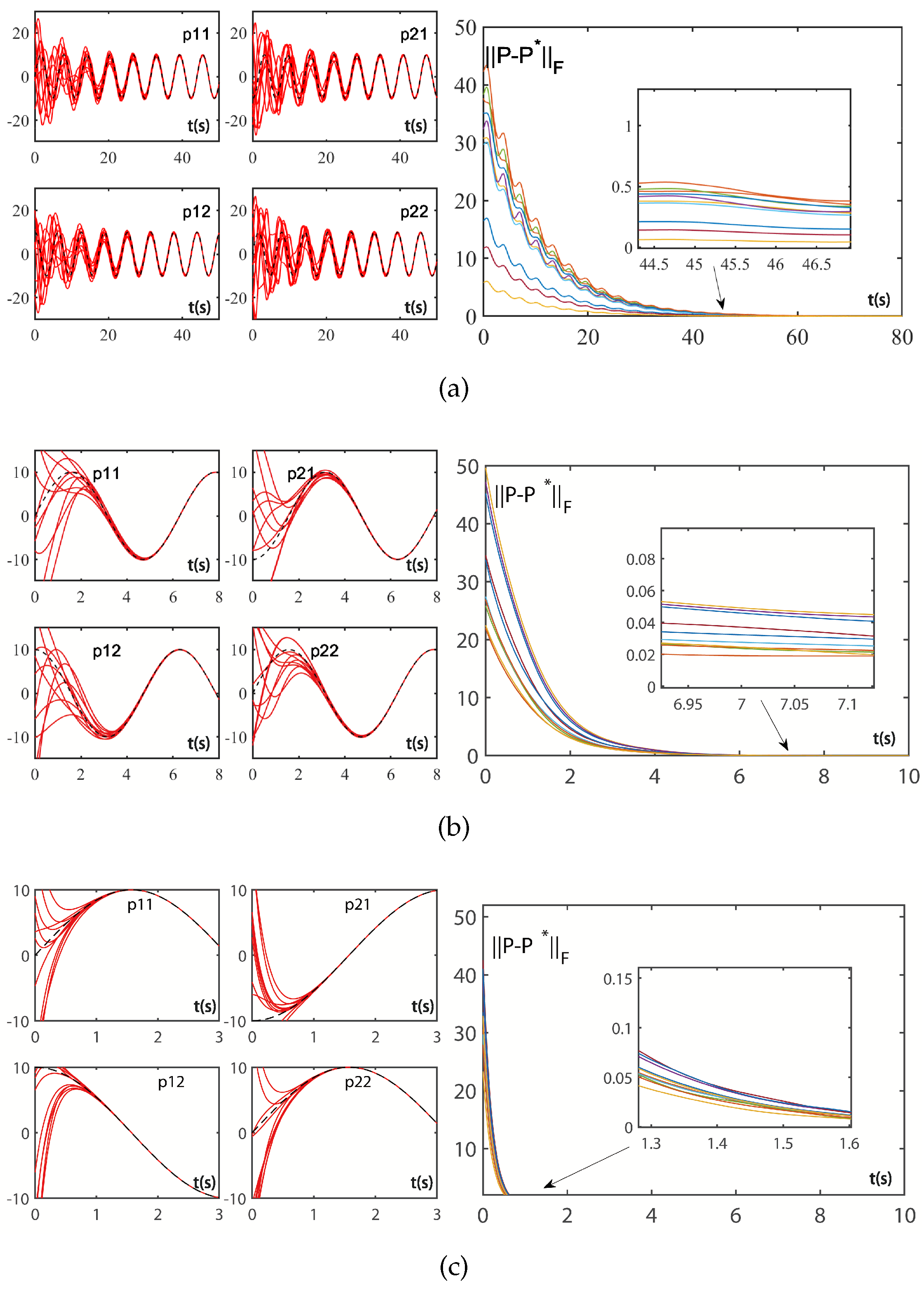
4.1. Convergence Discussion

In this section, we will discuss the convergence performance of the VFFTRNN and ZNN models in solving the Sylvester equation under various conditions.

First, we observe the effects of different factors on the convergence performance of ZNN and VFFTRNN with the same activation function.

Table 1. Comparisons of convergence time of ZNN and VFFTRNN when solving Sylvester equation.

Parameter $(\mathit{\alpha }=\mathit{\mu })$	${\mathit{T}}_{\mathit{ZNN}\left(\mathit{s}\right)}$	${\mathit{T}}_{\mathit{VFFTRNN}\left(\mathit{s}\right)}$
0.01	Cannot converge	2.39
0.1	67.55	2.25
0.2	34.20	1.99
0.5	13.88	1.69
1	6.98	1.41
2	3.48	1.02
5	1.37	0.49

presents a comparison of the convergence times of ZNN and VFFTRNN under various design factors.

Figure 2 and Figure 3 show detailed simulation results of both models under different conditions for $\alpha =\mu =0.1$, $\alpha =\mu =1$, and $\alpha =\mu =5$. As seen, when $\mu$ is sufficiently small (e.g., $\mu =0.01$), ZNN fails to converge. However, with $\mu =0.1$, the convergence time of ZNN is 67.55 s. As the design factor $\mu$ increases, the convergence performance of ZNN improves gradually. From Figure 2, we observe that when $\mu =1$, the computation error $\left|\right|P\left(t\right)-P^{*}\left(t\right){\left|\right|}_F$ converges to zero in 6.98 s, nearly ten times faster than with $\mu =0.1$. When $\mu =5$, the convergence time further decreases to just 1.37 s.

Next, we examine the convergence time of the computation error using VFFTRNN. With $\alpha =0.01$ or $\alpha =0.1$, the computation error $\left|\right|P\left(t\right)-P^{*}\left(t\right){\left|\right|}_F$ converges to zero in just 2.39 or 2.35 s, which is significantly faster than ZNN.

Furthermore, the comparison results in Table 1 and Figure 2 and Figure 3 clearly show that the convergence performance of VFFTRNN is significantly better than that of ZNN. It is worth noting that these simulation results use a linear-type activation function.

Second, we observed the effects of different activation functions on the convergence performance of ZNN and VFFTRNN when the same factors were set.

Figure 4 and Figure 5 show the computation error $\left|\right|P\left(t\right)-P^{*}\left(t\right){\left|\right|}_F$ curves for ZNN and VFFTRNN under three activation functions (i.e., linear, bipolar-sigmoid, and power-type).

When using the linear activation function, it can be observed that ZNN takes 6.98 s to converge to zero, whereas VFFTRNN converges in just 1.05 s. Similarly, when the bipolar-sigmoid or power activation functions are used, the convergence time of VFFTRNN is significantly shorter than that of ZNN.

This demonstrates the superior performance of the VFFTRNN system compared to ZNN and also verifies its finite-time convergence property for solving the Sylvester equation under different activation functions. It is worth noting that the factors were set to $\mu =\alpha =1$ and $\lambda ={\displaystyle \frac{1}{5}}$ in the above simulation results.

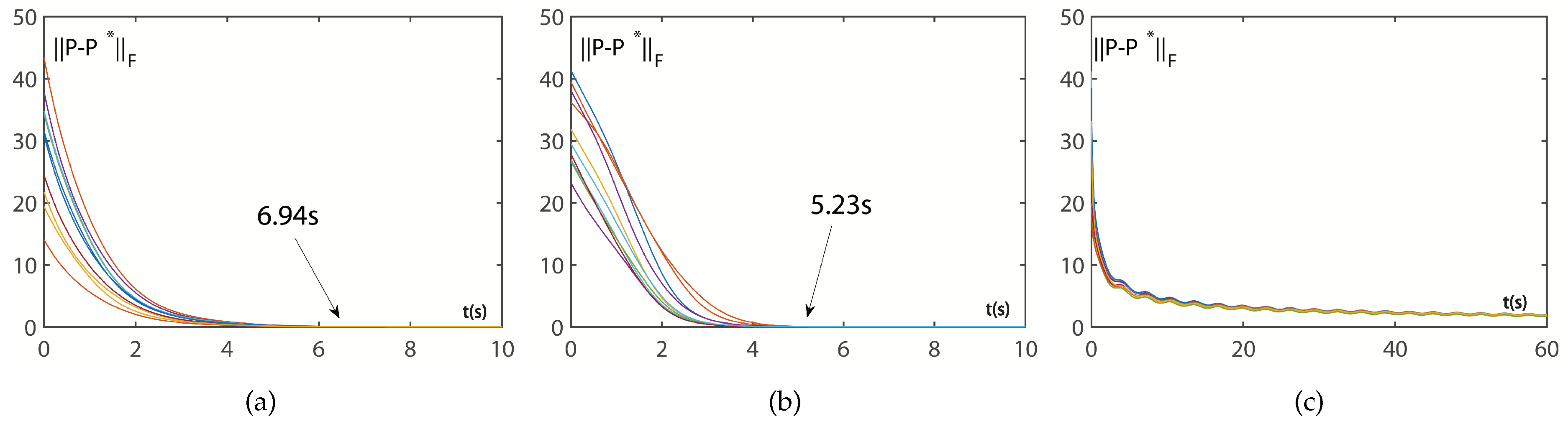
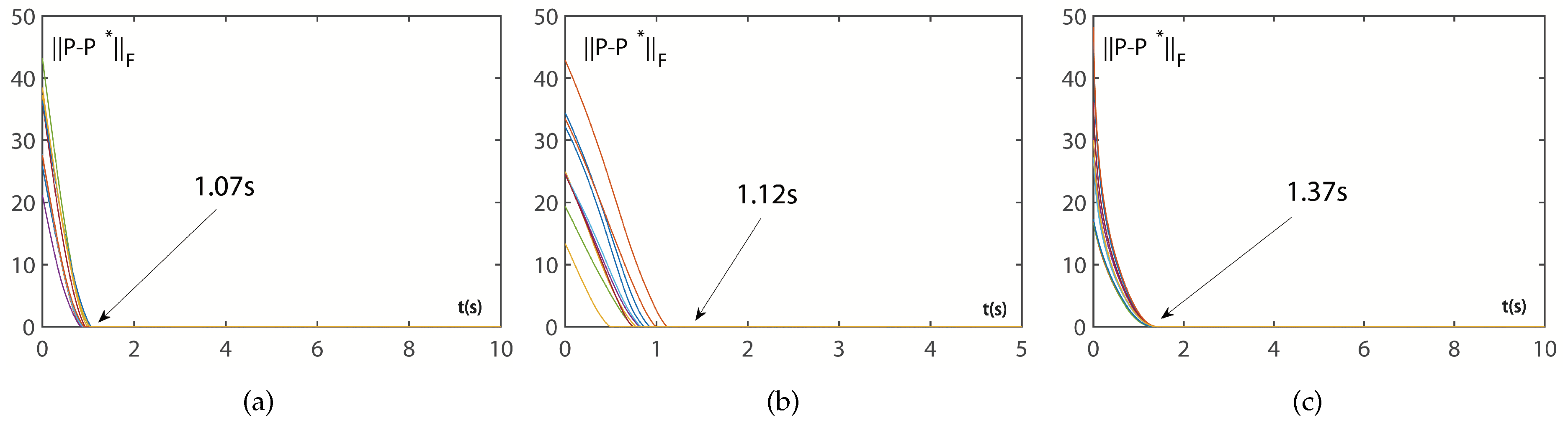
4.2. Robustness Discussion

In this section, we will verify the robustness of the VFFTRNN and compare it with the ZNN. To ensure both generality and simplicity, we consider the effects of differentiation and model implementation errors. For the simulation, we set the differentiation and model implementation errors as follows:

$$\begin{array}{cc}\hfill & \Lambda \left(t\right)={\beta }_1\left[\begin{array}{cc}\cos 2t& 0\\ 0& \sin 2t\end{array}\right],\Omega \left(t\right)={\beta }_2\left[\begin{array}{cc}0& \cos 2t\\ \sin 2t& 0\end{array}\right]\hfill \\ \hfill & \Delta \left(t\right)={\beta }_3\left[\begin{array}{cc}\sin 2t& 0\\ 0& \cos 2t\end{array}\right].\hfill \end{array}$$

where ${\beta }_1$, ${\beta }_2$ and ${\beta }_3$ are adjustable factors that control the magnitude of these disturbances.

In this section, we will compare the robustness of VFFTRNN and ZNN using the four cases shown in Figure 6. From Figure 6, it can be observed that when ${\beta }_1={\beta }_2={\beta }_3$, the disturbances are small, but the computation error $\left|\right|P\left(t\right)-P^{*}\left(t\right){\left|\right|}_F$ of ZNN does not converge to zero. In contrast, for VFFTRNN, we can see that the computation error converges within approximately 4 s.

Examining the other three cases, it is evident that the computation error of VFFTRNN still converges to zero, even with much larger disturbances. Notably, the convergence time of VFFTRNN decreases as the design factor $\alpha$ increases or $\lambda$ decreases.

In conclusion, although the presence of disturbances can affect the convergence performance of VFFTRNN, it still converges to zero in finite time, regardless of the size of the disturbance, confirming the robustness of the model.

5. Conclusions

In this paper, we propose a novel neural network called VFFTRNN and investigate its finite-time convergence and robustness for solving the Sylvester equation under three different activation functions. Compared to the conventional ZNN, the proposed VFFTRNN introduces a time-varying coefficient and a fractional power term, which accelerate the convergence speed. More importantly, VFFTRNN not only guarantees finite-time convergence but also achieves a super-exponential convergence rate. Simulation results demonstrate the superior performance of the proposed neural network in solving the Sylvester equation. Therefore, VFFTRNN offers significant advantages for real hardware implementation.

In the future, for hardware implementation, we will consider using FPGA to implement VFFTRNN networks. The flexibility and parallel processing capabilities of FPGA make it highly suitable for real-time applications, enabling efficient computation of network operations. This method will help achieve high performance and low power consumption, making it a feasible solution for the practical deployment of VFFTRNN networks.

References

1. Wei, Q.; Dobigeon, N.; Tourneret, J.Y.; Bioucas-Dias, J.; Godsill, S. R-FUSE: Robust fast fusion of multiband images based on solving a Sylvester equation. IEEE Signal Process. Lett. 2016, 23, 1632–1636. [Google Scholar] [CrossRef]
2. Wang, L.; Li, D.; He, T.; Xue, Z. Manifold regularized multi-view subspace clustering for image representation. In Proceedings of the 2016 23rd International Conference on Pattern Recognition (ICPR), Cancun, Mexico, 4–8 December 2016; IEEE: Piscataway, NJ, USA, 2016; pp. 283–288. [Google Scholar]
3. Hu, H.; Lin, Z.; Feng, J.; Zhou, J. Smooth representation clustering. In Proceedings of the IEEE Conference on Computer Vision and Pattern Recognition, Columbus, OH, USA, 23–28 June 2014; IEEE: Piscataway, NJ, USA, 2014; pp. 3834–3841. [Google Scholar]
4. Jang, J.S.; Lee, S.Y.; Shin, S.Y. An optimization network for matrix inversion. In Neural Information Processing Systems; MIT Press: Cambridge, MA, USA, 1987. [Google Scholar]
5. Fa-Long, L.; Zheng, B. Neural network approach to computing matrix inversion. Appl. Math. Comput. 1992, 47, 109–120. [Google Scholar] [CrossRef]
6. Cichocki, A.; Unbehauen, R. Neural networks for solving systems of linear equations and related problems. IEEE Trans. Circuits Syst. I Fundam. Theory Appl. 1992, 39, 124–138. [Google Scholar] [CrossRef]
7. Xia, Y.; Wang, J. A recurrent neural network for solving linear projection equations. Neural Netw. 2000, 13, 337–350. [Google Scholar] [CrossRef]
8. Zhang, Y.; Wang, J. Recurrent neural networks for nonlinear output regulation. Automatica 2001, 37, 1161–1173. [Google Scholar] [CrossRef]
9. Li, S.; Li, Y. Nonlinearly activated neural network for solving time-varying complex Sylvester equation. IEEE Trans. Cybern. 2013, 44, 1397–1407. [Google Scholar] [CrossRef] [PubMed]
10. Xiao, L.; Liao, B.; Luo, J.; Ding, L. A convergence-enhanced gradient neural network for solving Sylvester equation. In Proceedings of the 2017 36th Chinese Control Conference (CCC), Dalian, China, 26–28 July 2017; IEEE: Piscataway, NJ, USA, 2017; pp. 3910–3913. [Google Scholar]
11. Zhang, Z.; Zheng, L.; Weng, J.; Mao, Y.; Lu, W.; Xiao, L. A new varying-parameter recurrent neural-network for online solution of time-varying Sylvester equation. IEEE Trans. Cybern. 2018, 48, 3135–3148. [Google Scholar] [CrossRef]
12. Zhang, Y.; Jiang, D.; Wang, J. A recurrent neural network for solving Sylvester equation with time-varying coefficients. IEEE Trans. Neural Netw. 2002, 13, 1053–1063. [Google Scholar] [CrossRef]
13. Yan, X.; Liu, M.; Jin, L.; Li, S.; Hu, B.; Zhang, X.; Huang, Z. New zeroing neural network models for solving nonstationary Sylvester equation with verifications on mobile manipulators. IEEE Trans. Ind. Inform. 2019, 15, 5011–5022. [Google Scholar] [CrossRef]
14. Zhang, Z.; Zheng, L. A complex varying-parameter convergent-differential neural-network for solving online time-varying complex Sylvester equation. IEEE Trans. Cybern. 2018, 49, 3627–3639. [Google Scholar] [CrossRef]
15. Deng, J.; Li, C.; Chen, R.; Zheng, B.; Zhang, Z.; Yu, J.; Liu, P.X. A Novel Variable-Parameter Variable-Activation-Function Finite-Time Neural Network for Solving Joint-Angle Drift Issues of Redundant-Robot Manipulators. IEEE/ASME Trans. Mechatron. 2024, 1–12. [Google Scholar] [CrossRef]
16. Xu, X.; Sun, J.; Endo, S.; Li, Y.; Benjamin, S.C.; Yuan, X. Variational algorithms for linear algebra. Sci. Bull. 2021, 66, 2181–2188. [Google Scholar] [CrossRef] [PubMed]
17. Li, Y.; Chen, W.; Yang, L. Multistage linear gauss pseudospectral method for piecewise continuous nonlinear optimal control problems. IEEE Trans. Aerosp. Electron. Syst. 2021, 57, 2298–2310. [Google Scholar] [CrossRef]
18. Wang, X.; Liu, J.; Qiu, T.; Mu, C.; Chen, C.; Zhou, P. A real-time collision prediction mechanism with deep learning for intelligent transportation system. IEEE Trans. Veh. Technol. 2020, 69, 9497–9508. [Google Scholar] [CrossRef]
19. Zhang, Z.; Li, S.; Zhang, X. Simulink comparison of varying-parameter convergent-differential neural-network and gradient neural network for solving online linear time-varying equations. In Proceedings of the 2016 12th World Congress on Intelligent Control and Automation (WCICA), Guilin, China, 12–15 June 2016; pp. 887–894. [Google Scholar]
20. Zhang, Y.; Chen, D.; Guo, D.; Liao, B.; Wang, Y. On exponential convergence of nonlinear gradient dynamics system with application to square root finding. Nonlinear Dyn. 2015, 79, 983–1003. [Google Scholar] [CrossRef]
21. Wang, S.; Dai, S.; Wang, K. Gradient-based neural network for online solution of lyapunov matrix equation with li activation function. In Proceedings of the 4th International Conference on Information Technology and Management Innovation, Shenzhen, China, 12–13 September 2015; Atlantis Press: Amsterdam, The Netherlands, 2015; pp. 955–959. [Google Scholar]
22. Ma, W.; Zhang, Y.; Wang, J. Matlab simulink modeling and simulation of zhang neural networks for online time-varying sylvester equation solving. Comput. Math. Math. Phys. 2008, 47, 285–289. [Google Scholar]
23. Li, S.; Chen, S.; Liu, B. Accelerating a recurrent neural network to finite-time convergence for solving time-varying sylvester equation by using a sign-bi-power activation function. Neural Process. Lett. 2013, 37, 189–205. [Google Scholar] [CrossRef]
24. Shen, Y.; Miao, P.; Huang, Y.; Shen, Y. Finite-time stability and its application for solving time-varying sylvester equation by recurrent neural network. Neural Process. Lett. 2015, 42, 763–784. [Google Scholar] [CrossRef]
25. Jin, L.; Zhang, Y.; Li, S.; Zhang, Y. Modified znn for time-varying quadratic programming with inherent tolerance to noises and its application to kinematic redundancy resolution of robot manipulators. IEEE Trans. Ind. Electron. 2016, 63, 6978–6988. [Google Scholar] [CrossRef]
26. Mao, M.; Li, J.; Jin, L.; Li, S.; Zhang, Y. Enhanced discrete-time zhang neural network for time-variant matrix inversion in the presence of bias noises. Neurocomputing 2016, 207, 220–230. [Google Scholar] [CrossRef]
27. Xiao, L.; Liao, B. A convergence-accelerated zhang neural network and its solution application to lyapunov equation. Neurocomputing 2016, 193, 213–218. [Google Scholar] [CrossRef]
28. Liao, B.; Zhang, Y.; Jin, L. Taylor discretization of znn models for dynamic equality-constrained quadratic programming with application to manipulators. Neural Netw. Learn. Syst. IEEE Trans. 2016, 27, 225–237. [Google Scholar] [CrossRef] [PubMed]
29. Xiao, L. A finite-time convergent zhang neural network and its application to real-time matrix square root finding. Neural Comput. Appl. 2017, 31, 793–800. [Google Scholar] [CrossRef]
30. Zhang, Y.; Mu, B.; Zheng, H. Link between and comparison and combination of zhang neural network and quasi-newton bfgs method for time-varying quadratic minimization. IEEE Trans. Cybern. 2013, 43, 490–503. [Google Scholar] [CrossRef]
31. Yan, D.; Li, C.; Wu, J.; Deng, J.; Zhang, Z.; Yu, J.; Liu, P.X. A novel error-based adaptive feedback zeroing neural network for solving time-varying quadratic programming problems. Mathematics 2024, 12, 2090. [Google Scholar] [CrossRef]
32. Zhang, Z.; Lu, Y.; Zheng, L.; Li, S.; Yu, Z.; Li, Y. A new varying-parameter convergent-differential neural-network for solvingtime-varying convex QP problem constrained by linear-equality. IEEE Trans. Autom. Control 2018, 63, 4110–4125. [Google Scholar] [CrossRef]
33. Horn, R.A.; Johnson, C.R. Topics in Matrix Analysis, 1991; Cambridge University Presss: Cambridge, UK, 1991; Volume 37, p. 39. [Google Scholar]
34. Strang, G.; Freund, L. Introduction to applied mathematics. J. Appl. Mech. 1986, 53, 480. [Google Scholar] [CrossRef]
35. Mead, C.; Ismail, M. Analog VLSI Implementation of Neural Systems; Springer Science & Business Media: Berlin/Heidelberg, Germany, 2012; Volume 80. [Google Scholar]
36. Zhang, Y.; Ruan, G.; Li, K.; Yang, Y. Robustness analysis of the zhang neural network for online time-varying quadratic optimization. J. Phys. A Math. Theor. 2010, 43, 245202. [Google Scholar] [CrossRef]
Figure 1. Block diagram of VFFTRNN model ( 8 ) for solving the Sylvester equation.
Mathematics 12 03891 g001
Figure 2. Solving Sylvester Equation (1) with given coefficients online with ZNN and its computational error | | P ( t ) P * ( t ) | | F . Several red solid curves represent different initial states while the unique black dotted curve represents the theoretical solution. (a) Solution to ZNN with μ = 0.1 and error | | P ( t ) P * ( t ) | | F of ZNN with μ = 0.1 . (b) Solution to ZNN with μ = 1 and error | | P ( t ) P * ( t ) | | F of ZNN with μ = 1 . (c) Solution to ZNN with μ = 5 and error | | P ( t ) P * ( t ) | | F of ZNN with μ = 5 .
Mathematics 12 03891 g002
Figure 3. Solving Sylvester Equation (1) with given coefficients online with VFFTRNN and its computational error | | P ( t ) P * ( t ) | | F ( λ = 5 7 ). Several red solid curves represent different initial states while the unique black dotted curve represents the theoretical solution. (a) Solution to VFFTRNN with α = 0.1 and error | | P ( t ) P * ( t ) | | F of VFFTRNN with α = 0.1 . (b) Solution to VFFTRNN with α = 1 and error | | P ( t ) P * ( t ) | | F of VFFTRNN with α = 1 . (c) Solution to VFFTRNN with α = 5 and error | | P ( t ) P * ( t ) | | F of VFFTRNN with α = 5 .
Mathematics 12 03891 g003
Figure 4. The curves in the figure represent the convergence errors under different initial conditions. When ZNN uses different activation functions without perturbation to solve Sylvester Equation (1), its convergence error | | P ( t ) P * ( t ) | | F is as shown above ( μ = 1 ). (a) Linear. (b) Sigmoid. (c) Power ( s = 3 ).
Mathematics 12 03891 g004
Figure 5. The curves in the figure represent the convergence errors under different initial conditions. WhenVFFTRNN uses different activation functions without perturbation to solve Sylvester Equation (1), its convergence error | | P ( t ) P * ( t ) | | F is as shown above ( α = 1 and λ = 1 5 ). (a) Linear. (b) Sigmoid. (c) Power ( s = 3 ).
Mathematics 12 03891 g005
Figure 6. Robustness of ZNN and VFFTRNN with varying degrees of differential error and model implementation error. The arrows point to the original location of the magnified detail in each figure. (a) β 1 = β 2 = β 3 = 0.05 . (b) β 1 = β 2 = 0.05 and β 3 = 0.15 . (c) β 1 = β 3 = 0.05 . and β 2 = 0.15 . (d) β 1 = 0.15 and β 2 = β 3 = 0.05 .
Mathematics 12 03891 g006