The Lognormal Distribution Is Characterized by Its Integer Moments

Abstract

The lognormal moment sequence is considered. Using the fractional moments technique, it is first proved that the lognormal has the largest differential entropy among the infinite positively supported probability densities with the same lognormal-moments. Then, relying on previous theoretical results on entropy convergence obtained by the authors concerning the indeterminate Stieltjes moment problem, the lognormal distribution is accurately reconstructed by the maximum entropy technique using only its integer moment sequence, although it is not uniquely determined by moments.

1. Introduction and Some Useful Tools

The random variable X follows the lognormal distribution with parameters $\mu \in \mathbb{R}$ and ${\sigma }^2>0$, say $X\sim LN(\mu ,{\sigma }^2)$, if X is absolutely continuous with values in ${\mathbb{R}}^{+}$ and has density function

$$LN\left(x\right)={\displaystyle \frac{1}{\sqrt{2\pi {\sigma }^2}x}}{e}^{-{\displaystyle \frac{1}{2{\sigma }^2}}{(ln\left(x\right)-\mu )}^2},x\ge 0,$$

(1)

with integer moments ${\mu }_k=e^{k\mu +{\displaystyle \frac{1}{2}}{k}^2{\sigma }^2}$ for $k=1,2,\cdots$.

The lognormal distribution can be defined as the probability distribution of a random variable X whose logarithm obeys the normal law of probability centered at $\mu$; moreover, it is believed by some that it is “as fundamental a distribution in statistics as the normal one” and thus a very useful distribution for representing variables that are the multiplicative product of many positive-valued independent factors. This follows from the central limit theorem, since X is a lognormal random variable equivalent to $ln\left(X\right)$ being a normal random variable.

The lognormal distribution has some nice properties. For example, the product of independent lognormal variables is still lognormal; furthermore, if X is a lognormal random variable, then $aX$, $1/X$ and $X^a$ are also lognormal for $a\ne 0$. Because of its importance, the lognormal distribution, including the problem of moments, has been studied intensively by many researchers and has a wide range of applications in the natural sciences and in fields such as finance, economics, political science, sociology, philology, biology, and physical and industrial processes. Interestingly, insurance losses data analysis is positive, and the distribution is often unimodal hump-shaped, right-skewed, and with heavy tails. Although many parametric unimodal distributions have been used in the actuarial literature to model these data, their characteristics require more flexible models. In particular, the losses in the right tail, although rare in frequency, are in fact those that have the greatest impact on an insurer’s operations and could lead to the possible bankruptcy of the company. In such circumstances, heavy-tailed distributions have been shown to be reasonably competitive. Different classes of models can be considered to select a suitable distribution. For example, ref. [1], Equation (3), have successfully considered a mode-parametrised unimodal Gamma distribution. And again, ref. [2], Equation (5) consider a mode-parameterized lognormal distribution. Special mention should be made of the famous paper by [3] which clearly demonstrated the moment non-uniqueness of a general lognormal distribution by explicitly writing an infinite family of different distributions all having the same moments as those of $LN(\mu ,{\sigma }^2)$. Integral transforms, such as the Laplace and Fourier transforms, of the lognormal distribution have received considerable attention in the literature for several decades. Since these integral transforms have no known closed form, considerable effort has been devoted to finding viable approximation methods. Recently, ref. [4] presented two parametric approximations (Theorems 3 and 4) for the Laplace transform of the lognormal distribution.

These approximations improve as this parameter goes to infinity and can be used for numerical calculations. Another characterization property of the lognormal distribution using the Kullback–Leibler measure $D(g,g_r)=:{\int }_{{\mathbb{R}}^{+}}g\left(x\right)ln{\displaystyle \frac{g\left(x\right)}{g_r\left(x\right)}}dx$ between the probability density functions g and its r size-weighted counterpart $g_r\left(x\right)={\displaystyle \frac{x^r}{{\mu }_r}}g\left(x\right)$, with finite moments ${\mu }_r=\mathbb{E}\left(X^r\right)<\infty$, for $r\in \mathbb{R}$, have been provided by [5], Theorem 1.

The authors claim that $D(g,g_r)$ becomes symmetric, i.e., $D(g,g_r)=D(g_r,g)$, if and only if g coincides with the lognormal density. Following [5], we want to give a further characterization of $LN(\mu ,{\sigma }^2)$ in the context of so-called fractional moments (see [6]) this will allow us to prove that the lognormal density has the largest entropy among all densities sharing the same moments.

From now on, for the sake of calculation simplicity, in place of the general $LN(\mu ,{\sigma }^2)$ distribution, we investigate the centered lognormal distribution $LN(0,{\sigma }^2)$. Note that all its properties and related results hold also for its non-centered (1).

Consider an indeterminate Stieltjes moment problem (books such as [7,8,9], are widely known references on this topic and contain exhaustive details on the debate and progress made in the moment problems for a century; for more recent results, see [10,11]. For determinacy/indeterminacy criteria of moment problem by means of the entropic technique, see [12].

Within the maximum entropy (MaxEnt, shortly) rationale, it is well known that $LN(0,{\sigma }^2)$ can be considered having the largest entropy among all positive random variables X with assigned expected values $\mathbb{E}[ln(X\left)\right]$ and $\mathbb{E}\left[{ln}^2\left(X\right)\right]$, respectively. This fact is not surprising in view of the maximal entropy property of the normal distribution once assigned $\mathbb{E}\left[X\right]$ and $\mathbb{E}\left[X^2\right]$ and taking into account the relationship between normal and lognormal distributions.

As a consequence, recalling the well-known fact that the logarithm function can be expressed as the pointwise limit of a sequence of simpler functions for every $x>0$ (see Equation (5) below), our goal will be realized by means of two distinct tools

(a)

Firstly by the so-called fractional moments which will allow us to prove the lognormal has the largest entropy out all densities having the lognormal moments (Theorem 2 below);

(b)

Then, by the so-called integer moments, which will allow us to prove, employing the complete sequence of integer moments solely, out densities having lognormal moments, the lognormal only may be reconstructed (Theorem 3 below). Equivalently, the lognormal is characterized by its integer moments, justifying the paper’s title, although it is not uniquely determined by lognormal moments.

The rest of the paper is structured as follows. In Section 2, it is proved that the lognormal distribution is characterized by two fractional moments $\mathbb{E}\left(X^{\alpha }\right)$ and $\mathbb{E}\left(X^{2\alpha }\right)$, with $\alpha \to 0^{+}$, and its entropy coincides with the entropy of $g_{hmax}$, which is the member of the class ${\mathcal{C}}_{\infty }$ with maximum entropy. In Section 3, the lognormal density is recovered by its integer moment sequence using the MaxEnt technique, and it is further shown that the sequence of entropies associated with the MaxEnt densities converges to the entropy of $g_{hmax}$ and hence, to the entropy of the lognormal distribution. Finally, by noting that the sequence of entropies of the MaxEnt densities is a Cauchy sequence, using its properties, it is concluded that the sequence of MaxEnt densities converges almost everywhere to the lognormal one. Section 4 will illustrate the so-called Askey density previously found in the literature and labeled as “another continuous weight function for the lognormal moments”. Finally, in Section 5, some charaterizations of the lognormal are listed.

2. Characterization of Lognormal via Fractional Moments

From [13], p.59, we preliminarily recall the following well-known result: the MaxEnt density $f_n^{fm}$ constrained by the n fractional moments ${\left\{\mathbb{E}\left(X^{{\alpha }_j}\right)\right\}}_1^n$, ${\alpha }_j>0$, and in addition to ${\alpha }_0=0$ and $\mathbb{E}\left(X^{{\alpha }_0}\right)=1$ for normalizing reasons, amounts to

$$f_n^{fm}\left(x\right)=e^{-{\sum }_0^n{\lambda }_j{x}^{{\alpha }_j}}$$

(2)

where ${\lambda }_0,{\lambda }_1,\cdots ,{\lambda }_n$, are the Lagrange multipliers calculated by imposing fractional moments

$${\int }_{{\mathbb{R}}^{+}}{x}^{{\alpha }_j}{f}_n^{fm}\left(x\right)dx=\mathbb{E}\left(X^{{\alpha }_j}\right),j=0,\cdots ,n$$

as constraints as stressed by the index $fm$, and the corresponding entropy is given by

$$H\left[f_n^{fm}\right]=\sum _{j=0}^n{\lambda }_j\mathbb{E}\left[X^{{\alpha }_j}\right].$$

(3)

For more theoretical and numerical details on the topic, see [6].

In an indeterminate Stieltjes moment problem, the totality of densities g with support ${\mathbb{R}}^{+}$ forms the convex set

$${\mathcal{C}}_{\infty }:=\left\{g\ge 0|{\int }_{{\mathbb{R}}^{+}}{x}^{k}g\left(x\right)dx={\mu }_k,k=0,1,\cdots \right\},$$

with some properties:

• In ${\mathcal{C}}_{\infty }$ there is a unique density, say $g_{hmax}$, having largest differential entropy (shortly, entropy), being the continuous entropy functional

  $$H:g\to H\left[g\right]=:\mathbb{E}[-ln\left(X\right)]=-{\int }_{{\mathbb{R}}^{+}}g\left(x\right)lng\left(x\right)dx$$

  strictly concave and, over the convex set ${\mathcal{C}}_{\infty }$, H takes a maximum $H\left[g_{hmax}\right]$. As a consequence, excluding $g_{hmax}$, every $g\in {\mathcal{C}}_{\infty }$ has entropy $H\left[g\right]<H\left[g_{hmax}\right]$ strictly.
• $LN(0,{\sigma }^2)$ belongs to ${\mathcal{C}}_{\infty }$, and in Theorem 2 below, the first main result will be proved, that is $H\left[LN(0,{\sigma }^2)\right]=H\left[g_{hmax}\right]$ and then $LN(0,{\sigma }^2)\equiv g_{hmax}$.

The following result, formalized in Lemma 1, is preliminary to the characterization of the lognormal distribution by fractional moments of appropriate order $\alpha \in {\mathbb{R}}^{+}$.

Lemma 1.

The lognormal may be equivalently considered as MaxEnt density having two characterizing fractional moments $\{\mathbb{E}\left(X^{\alpha }\right),\mathbb{E}\left(X^{2\alpha }\right)\}$, with $\alpha \to 0^{+}$.

Proof. 

From the elementary inequality for positive real number $e^y\ge 1+y$ the following one $1-{\displaystyle \frac{1}{y}}\le ln\left(y\right)\le y-1$ is drawn with equality if and only if $y=1$. Next, setting $y=x^{1/n}$, with $n\in \mathbb{N}$, for each $n\ge 1$ two additional inequalities

$$\left\{\begin{array}{cc}\hfill & 1-{\displaystyle \frac{1}{x}}\le ln\left(x\right)\le n(x^{1/n}-1)\le x^{1/n}ln\left(x\right)\le xln\left(x\right),\mathrm{if}x>0\hfill \\ \hfill & \\ \hfill & {\left[n(x^{1/n}-1)\right]}^2\le {ln}^2\left(x\right),\mathrm{if}0<x\le 1\hfill \end{array}\right.$$

(4)

involving $ln\left(x\right)$ and ${ln}^2\left(x\right)$ are drawn. As well recall the well-known fact that the logarithm function can be expressed as the pointwise limit of a sequence of simpler functions for every $x>0$

$$ln\left(x\right)=\underset{n\to \infty }{lim}n(x^{1/n}-1),{ln}^2\left(x\right)=\underset{n\to \infty }{lim}{\left[n(x^{1/n}-1)\right]}^2$$

(5)

Replacing in (1) $ln\left(x\right)$ and ${ln}^2\left(x\right)$ with $n(x^{1/n}-1)$ and ${\left[n(x^{1/n}-1)\right]}^2$, respectively, the continuous function sequence $\left\{L{N}_n\right\}\in {\mathcal{L}}_1[0,\infty )$ is drawn with

$$\begin{array}{c}\hfill L{N}_n\left(x\right)=e^{-{\displaystyle \frac{1}{2}}ln\left(2\pi {\sigma }^2\right)-n(x^{1/n}-1)-{\displaystyle \frac{1}{2{\sigma }^2}}{\left[n(x^{1/n}-1)\right]}^2}\\ \hfill =e^{-[{\displaystyle \frac{1}{2}}ln\left(2\pi {\sigma }^2\right)-n+{\displaystyle \frac{n^2}{2{\sigma }^2}}]-[n-{\displaystyle \frac{n^2}{{\sigma }^2}}]x^{1/n}-{\displaystyle \frac{n^2}{2{\sigma }^2}}{x}^{2/n}}\end{array}$$

(6)

Combining (4) with (6) allows us to concluding no entry $L{N}_n$ can be considered as probability density. From (5) and each fixed $x\in {\mathbb{R}}^{+}$, the integrable function sequence $\left\{L{N}_n\right\}$ is pointwise convergent to $LN$. Furthermore, $LN$ has mode $x_{\mathrm{mode}}=e^{-{\sigma }^2}$ with $LN\left(x_{\mathrm{mode}}\right)={\displaystyle \frac{e^{\frac{1}{2}{\sigma }^2}}{\sqrt{2\pi {\sigma }^2}}}$. From (6), each entry $L{N}_n$ admits a maximum at $x_n={(1-{\displaystyle \frac{{\sigma }^2}{n}})}^n\le e^{-{\sigma }^2}<1$ with $LN\left(x_n\right)=LN\left(x_{\mathrm{mode}}\right)$ independent on n, so that $\left\{L{N}_n\right\}$ is a sequence of positive, continuous, uniformly bounded, pointwisely convergent to $LN$ functions for all $x\in [0,\infty )$. From (1)–(6), we have

$$\left\{\begin{array}{cc}LN\left(x\right)\le L{N}_n\left(x\right)\hfill & \mathrm{if}0<x\le 1\hfill \\ \hfill & \\ LN\left(x\right)>L{N}_n\left(x\right)\hfill & \mathrm{if}x>1\hfill \end{array}\right.$$

(7)

Taking into account (4), the piecewise continuous function $\phi$ is defined as

$$\phi \left(x\right)=:\left\{\begin{array}{cc}LN\left(x_{\mathrm{mode}}\right)\hfill & \mathrm{if}0<x\le 1\hfill \\ \hfill & \\ LN\left(x\right)\hfill & \mathrm{if}x>1\hfill \end{array}\right.$$

(8)

In the next three items, the dominated convergence theorem will be used so that we need to construct a suitable positive piecewise continuous integrable function ${\phi }_1\left(x\right)$, $x\in [0,\infty )$ (the so-called dominating function).

• Assuming from (8) ${\phi }_1=\phi$, then $L{N}_n\left(x\right)\le {\phi }_1\left(x\right)$ for each $x\ge 0$ and each n, and ${\phi }_1\in {\mathcal{L}}_1[0,\infty )$ holds, so that all the requirements of the dominated convergence theorem are satisfied, from which it follows that

  $$\underset{n\to \infty }{lim}{\int }_{{\mathbb{R}}^{+}}L{N}_n\left(x\right)dx={\int }_{{\mathbb{R}}^{+}}LN\left(x\right)dx=1.$$

  (9)
• As above recalled, none of the entries of the positive function sequence $\left\{L{N}_n\right\}$ can be considered as density; hence, the sequence $\{H\left[L{N}_n\right]=:-{\int }_{{\mathbb{R}}^{+}}L{N}_n\left(x\right)ln\left(L{N}_n\left(x\right)\right)dx\}$ is improperly called an “entropy sequence”. Nevertheless, we will be able to prove that

  $$\underset{n\to \infty }{lim}H\left[L{N}_n\right]=-\underset{n\to \infty }{lim}{\int }_{{\mathbb{R}}^{+}}L{N}_n\left(x\right)ln\left(L{N}_n\left(x\right)\right)dx=-{\int }_{{\mathbb{R}}^{+}}LN\left(x\right)ln\left(LN\left(x\right)\right)dx=H\left[LN\right].$$

  (10)
  Indeed, consider (6), from which

  $$\begin{array}{cc}\hfill H\left[L{N}_n\right]& =-{\int }_{{\mathbb{R}}^{+}}L{N}_n\left(x\right)ln(L{N}_n\left(x\right)dx\hfill \\ \hfill & =-{\int }_{{\mathbb{R}}^{+}}\left[{\displaystyle \frac{1}{2}}ln\left(2\pi {\sigma }^2\right)+n(x^{1/n}-1)+{\displaystyle \frac{1}{2{\sigma }^2}}{\left[n(x^{1/n}-1)\right]}^2\right]L{N}_n\left(x\right)dx\hfill \end{array}$$
  Split just above integral ${\int }_{{\mathbb{R}}^{+}}$ into ${\int }_0^1+{\int }_1^{\infty }$, take into account (4), (7) and (8); then, find the upper bound for the sequence $\{L{N}_{n}ln\left(L{N}_n\right)\}$

  $$\begin{array}{cc}\hfill \mid L{N}_n\left(x\right)ln\left(L{N}_n\left(x\right)\right)\mid & =\mid {\displaystyle \frac{1}{2}}ln\left(2\pi {\sigma }^2\right)+n(x^{1/n}-1)+{\displaystyle \frac{1}{2{\sigma }^2}}{\left[n(x^{1/n}-1)\right]}^2\mid L{N}_n\left(x\right)\hfill \\ \hfill & \le (\mid {\displaystyle \frac{1}{2}}ln\left(2\pi {\sigma }^2\right)\mid +\mid n(x^{1/n}-1)\mid +{\displaystyle \frac{1}{2{\sigma }^2}}{\left[n(x^{1/n}-1)\right]}^2)L{N}_n\left(x\right)\hfill \end{array}$$

  from which arises the piecewise continuous and integrable dominating function

  $${\phi }_2\left(x\right)=\left\{\begin{array}{c}\left({\displaystyle \frac{1}{2}}\mid ln\left(2\pi {\sigma }^2\right)\mid -ln\left(x\right)+{\displaystyle \frac{1}{2{\sigma }^2}}{ln}^2\left(x\right)\right)LN\left(x_{\mathrm{mode}}\right),\mathrm{if}x\le 1\hfill \\ \hfill & \\ \left({\displaystyle \frac{1}{2}}\mid ln\left(2\pi {\sigma }^2\right)\mid +xln\left(x\right)+{\displaystyle \frac{1}{2{\sigma }^2}}{ln}^2\left(x\right)\right)LN\left(x\right),\mathrm{if}x>1\hfill \end{array}\right.$$

  and then $\mid L{N}_{n}log\left(L{N}_n\right)\mid \le {\phi }_2\in {\mathcal{L}}_1[0,\infty )$ for each n. Consequently, from the dominated convergence theorem, (10) is proved.
• A similar result holds for the moment curves of $LN$

  $$m_{LN}\left(\alpha \right)={\int }_{{\mathbb{R}}^{+}}{x}^{\alpha }LN\left(x\right)dx=e^{{\displaystyle \frac{1}{2}}{\sigma }^2{\alpha }^2}$$

  and of $L{N}_n$

  $$m_{L{N}_n}\left(\alpha \right)={\int }_{{\mathbb{R}}^{+}}{x}^{\alpha }L{N}_n\left(x\right)dx$$

  for each $n\ge 1$, with $\alpha \ge 0$. Combining item 1 with (8), we know each $L{N}_n\le {\phi }_1$, from which each sequence entry $\left\{x^{\alpha }L{N}_n\right\}\le x^{\alpha }{\phi }_1$. As a consequence, the function ${\phi }_3=x^{\alpha }{\phi }_1$ for each $\alpha \ge 0$ satisfies ${\int }_{{\mathbb{R}}^{+}}{\phi }_3\left(x\right)dx<\infty$ and, being piecewise continuous, is the required dominating function. For each $\alpha \ge 0$, the following relationship follows

  $$\underset{n\to \infty }{lim}{m}_{L{N}_n}\left(\alpha \right)=\underset{n\to \infty }{lim}{\int }_{{\mathbb{R}}^{+}}{x}^{\alpha }L{N}_n\left(x\right)dx={\int }_{{\mathbb{R}}^{+}}{x}^{\alpha }LN\left(x\right)dx=m_{LN}\left(\alpha \right)$$

  (11)

  Combining (6)–(11) and replacing ${\displaystyle \frac{1}{n}}$ with $\alpha$ in (6), it can be concluded that the lognormal has to be considered MaxEnt distribution characterized by two fractional moments $\{\mathbb{E}\left(X^{\alpha }\right),\mathbb{E}\left(X^{2\alpha }\right)\}$ with $\alpha \to 0^{+}$. Then, Lemma 1 is proved.

□

Just to have an idea about how well $L{N}_n$ given in (6) approximates the $LN$ density, look at the following graph (Figure 1).

Here (top), as n increases ${sup}_x\mid LN-L{N}_n\mid$ tends to zero exponentially, leaving to presume that $L{N}_n$ is uniformly convergent to $LN$. Consequently (bottom), the difference $(LN-L{N}_n)$ tends to zero uniformly. The order of magnitude of the error made gives an idea of how well $L{N}_n$ approximates $LN$.

Lemma 1 allows us to reconnect to the fractional moments problem in the MaxEnt framework; in this setup, a crucial role is played by the following distribution characterization theorem, hereafter referred to as Lin’s theorem, due to Lin (1992).

Theorem 1

([14]). A positive r.v. X is uniquely characterized by an infinite sequence of positive fractional moments ${\left\{\mathbb{E}\left(X^{{\alpha }_j}\right)\right\}}_1^{\infty }$ with distinct exponents ${\alpha }_j\in (0,{\alpha }^{*})$, $\mathbb{E}\left(X^{{\alpha }^{*}}\right)<\infty$, for some ${\alpha }^{*}>0$.

Similarly, it can be shown that several other distributions, such as Gamma, generalized Gamma, Weibull, Rayleigh, Chi-Square, and Pareto, to name a few, can be considered as MaxEnt distributions characterized by a few fractional moments.

We are now able to demonstrate the first main result of this paper by means of the fractional moments technique.

Theorem 2

(Main Result-I). Of all the densities $g\in {\mathcal{C}}_{\infty }$ with lognormal moments, the lognormal $LN$ has the largest entropy, that is

$$H\left[LN\right]={\mathit{max}}_{g\in {\mathcal{C}}_{\infty }}H\left[g\right]=H\left[g_{hmax}\right]$$

(12)

so that $LN$ coincides with $g_{hmax}$.

Proof. 

For an arbitrary $g\in {\mathcal{C}}_{\infty }$, consider its moment curve $m_g\left(\alpha \right)={\int }_{{\mathbb{R}}^{+}}{x}^{\alpha }g\left(x\right)dx$. In general, $m_g\left(\alpha \right)\ne m_{LN}\left(\alpha \right)$ except when $\alpha =j$, $j=0,1,2,...$; in which case $m_g\left(j\right)=m_{LN}\left(j\right)={\mu }_j$ holds. Let $f_2^{fm}$ be the MaxEnt approximation of g, constrained by two fractional moments $\{\mathbb{E}\left(X^{\alpha }\right),\mathbb{E}\left(X^{2\alpha }\right)\}$ picked up from $m_g\left(\alpha \right)$, with small and fixed $\alpha$. Thanks to (11), the couple of values follows $\{\mathbb{E}\left(X^{\alpha }\right),\mathbb{E}\left(X^{2\alpha }\right)\}\in m_g\left(\alpha \right)\simeq \{\mathbb{E}\left(X^{\alpha }\right),\mathbb{E}\left(X^{2\alpha }\right)\}\in m_{LN}\left(\alpha \right)$. Recalling the entropy $H\left[g\right]$ of an arbitrary density g is a continuous function of two expected values $\{\mathbb{E}\left(X^{\alpha }\right),\mathbb{E}\left(X^{2\alpha }\right)\}\in m_g\left(\alpha \right)$, thanks to (10), the relationship $H\left[LN\right]\simeq H\left[f_2^{fm}\right]$ can be set. Now, consider an arbitrary $g\in {\mathcal{C}}_{\infty }$, its moment curve $m_g\left(\alpha \right)$ and a sequence of its fractional moments $\{\mathbb{E}\left(X^{\alpha }\right),\mathbb{E}\left(X^{2\alpha }\right),\left\{\mathbb{E}{\left(X^{{\alpha }_j}\right\}}_3^{\infty }\right\}$ satisfying Lin’s theorem conditions, with fixed small $\alpha$ and each ${\alpha }_j>2\alpha$. For each $g\in {\mathcal{C}}_{\infty }$, with $g\ne g_{hmax}$, it holds

$$H\left[LN\right]\simeq H\left[f_2^{fm}\right]>H\left[g\right]$$

(13)

as the couple $\{\mathbb{E}\left(X^{\alpha }\right),\mathbb{E}\left(X^{2\alpha }\right)\}\in m_{LN}\left(\alpha \right)$, with $\alpha \to 0^{+}$, characterizes $LN$, in contrast to the couple $\{\mathbb{E}\left(X^{\alpha }\right),\mathbb{E}\left(X^{2\alpha }\right)\}\in m_g\left(\alpha \right)\simeq \{\mathbb{E}\left(X^{\alpha }\right),\mathbb{E}\left(X^{2\alpha }\right)\}\in m_{LN}\left(\alpha \right)$, with $\alpha \to 0^{+}$, which does not characterize any of the remaining $g\in {\mathcal{C}}_{\infty }$. So, $H\left[LN\right]=H\left[g_{hmax}\right]>H\left[g\right]$ holds for every $g\in {\mathcal{C}}_{\infty }$; combining the uniqueness of $g_{hmax}$ in ${\mathcal{C}}_{\infty }$ with the fact that $LN\in {\mathcal{C}}_{\infty }$ too, it follows $LN\equiv g_{hmax}$. Consequently, Theorem 2 is proved. □

3. Characterization and Reconstruction of Lognormal via Its Integer Moments

Given that the moment problem for the lognormal density is indeterminate, one might expect that approximations based uniquely on a sequence of integer moments might either fail to converge or converge to a different distribution with the same moments. A difficult proof would no doubt be required, and perhaps a similar approximation might be numerically very unstable for more than a few moments. Theorem 2 allows us to solve the problem. Suppose in a positive distribution reconstruction process only the whole moment sequence is known, specifically the lognormal moments $\{{\mu }_k=e^{{\displaystyle \frac{1}{2}}{\sigma }^2{k}^2}{\}}_1^{\infty }$.

The question follows: using the MaxEnt method with lognormal moments as constraints, which distribution is reconstructed (in other words, identified or characterized) out of the infinitely many candidate distributions belonging to ${\mathcal{C}}_{\infty }$? The expected answer is obvious: the one with the largest entropy.

Considering an indeterminate Stieltjes moment problem, [15] - Thm. 7, have indeed shown that the MaxEnt approximation converges in entropy to $g_{hmax}$ and, in combination with the Theorem 2, gives us the relation

$$\underset{n\to \infty }{lim}H\left[f_n^{im}\right]=H\left[g_{hmax}\right]=H\left[LN\right].$$

(14)

Here, the index $im$ refers to the fact that $f_n^{im}\left(x\right)=e^{-{\sum }_0^n{\lambda }_j{x}^j}$ is the MaxEnt approximation of the lognormal density based on using integer moments as constraints and having an analytical form analogous to (2), in which the term ${\alpha }_j$ is replaced by j.

In addition to the convergence in the entropy (14), the following also holds true.

Theorem 3

(Main Result-II). The sequence $\left\{f_n^{im}\left(x\right)\right\}$ converges a.e. to $LN$ in ${\mathcal{L}}_1$

$$\underset{n\to \infty }{lim}{f}_n^{im}=LNa.e.$$

so that $g_{hmax}=LN$ almost everywhere. Equivalently, LN is characterized by the sequence of its integer moments.

Proof. 

The proof is obtained combining together the following facts.

• [15] - Thm. 7, proved that the monotonically non-increasing sequence $\left\{H\left[f_n^{im}\right]\right\}$ converges to the quantity $H\left[g_{hmax}\right]=H\left[LN\right]$ finite, so that taking into account (14), $\left\{H\left[f_n^{im}\right]\right\}$ is a Cauchy sequence.
• Consider the Kullback–Leibler distance between densities $LN$ and $f_n^{im}$

  $$D_{KL}(LN,f_n^{im}):={\int }_{{\mathbb{R}}^{+}}LN\left(x\right)ln{\displaystyle \frac{LN\left(x\right)}{f_n^{im}\left(x\right)}}dx$$
  As $LN$ and $f_n^{im}$ share the same first n moments ${\left\{{\mu }_k\right\}}_1^n$, the relationship below easily follows:

  $${\int }_{{\mathbb{R}}^{+}}LN\left(x\right)ln{\displaystyle \frac{LN\left(x\right)}{f_n^{im}\left(x\right)}}dx=H\left[f_n^{im}\right]-H\left[LN\right].$$

  (15)
• Recall Pinsker’s inequality ([16], p. 390),

  $${\displaystyle \frac{1}{2}}{\Vert f_n^{im}-LN\Vert }_1^2\le D_{KL}(LN,f_n^{im})$$
  Collecting together items 1–3, Equation (15) and $m>n$ arbitrary indices, it follows

  $${\displaystyle \frac{1}{2}}{\Vert f_n^{im}-f_m^{im}\Vert }_1^2\le D_{KL}(f_m^{im},f_n^{im})=H\left[f_n^{im}\right]-H\left[f_m^{im}\right]$$

  so that $\left\{f_n^{im}\right\}$ is a Cauchy sequence in ${\mathcal{L}}_1$.
• $LN$ is the unique density in ${\mathcal{C}}_{\infty }$ with the largest entropy value $H\left[LN\right]=H\left[g_{hmax}\right]$. Replacing $f_m^{im}$ with $LN$, letting $n\to \infty$, recalling (14), the completeness of ${\mathcal{L}}_1$ and the items 1–3

  $${\displaystyle \frac{1}{2}}{\Vert f_n^{im}-LN\Vert }_1^2\le D_{KL}(LN,f_n^{im})=H\left[f_n^{im}\right]-H\left[LN\right]\to 0$$

  so that $\left\{f_n^{im}\right\}$ is uniformly convergent to $LN$. It is standard that $\left\{f_n^{im}\right\}$ has a subsequence pointwise convergent a.e. to $g_{hmax}=LN$ and the sequence itself converges a.e. to the same limit, which could explain the goodness of the approximation of $LN$ through the MaxEnt approximation $f_n^{im}$ based on integer moments.

□

4. Askey and Berg Densities Having Lognormal Moments

In the previous section, we showed that among the infinitely many densities in ${\mathcal{C}}_{\infty }$, the lognormal $LN$ has the largest entropy. To our knowledge, there are two other densities in ${\mathcal{C}}_{\infty }$, excluding the so-called Stieltjes classes (see [17]), $\omega$ and ${\omega }_c$, called Askey and Berg densities, respectively: we now want to investigate the connection between $LN$ and $\omega$. Theorem 3 gives us the opportunity to study the Askey density $\omega$, which is considered in the literature as different from $LN$ for the simple reason that this has a different analytical form. It might also be interesting to represent $LN$ by an analytical expression in which the full sequence ${\left\{{\mu }_k\left\{LN\right\}\right\}}_1^{\infty }$ of the lognormal moments appears explicitly, which is consistent with the fact that $g_{hmax}=LN$, since only the latter is characterized by the lognormal moment sequence.

In order to achieve this, the following three facts are brought together.

• From Theorem 3, $g_{hmax}=LN$ holds a.e.;
• [18] - Theorem 2.1, considered Jacobi’s theta function

  $${\mathrm{\Theta }}_q\left(x\right):=\sum _{-\infty }^{\infty }{x}^k{q}^{{\displaystyle \frac{1}{2}}{k}^2},x>0$$

  (16)

  where $q=exp(-{\sigma }^2)$, so that $0<q<1$ and proved, as $q\to 1^{-}$,

  $${\mathrm{\Theta }}_q\left(x\right)\underset{a}{=}\sqrt{{\displaystyle \frac{2\pi }{ln(1/q)}}}{e}^{{\displaystyle \frac{{ln}^2\left(x\right)}{2ln(1/q)}}}$$

  (17)
  Here, the symbol “$\underset{a}{=}$” means asymptotically equal; that is, we write $A_q\underset{a}{=}{B}_q$ if ${lim}_{q\to 1^{-}}{A}_q/B_q=1$.
• Askey and Berg (see [19], Equations (2.5) and (2.8) for details and further references), respectively, found the densities

  $$\omega \left(x\right)={\displaystyle \frac{1}{ln(1/q)·x·{\mathrm{\Theta }}_q\left(x\right)}}$$

  (18)

  and its one-parameter extension

  $${\omega }_c\left(x\right)={\displaystyle \frac{x^{c-1}}{M_c{\mathrm{\Theta }}_q\left(x{q}^{-c}\right)}}$$

  (19)
  The last one satisfies the property ${\omega }_{c+1}={\omega }_c$ with $M_c$ as the normalizing constant and $M_{c+1}=q^{c+1/2}{M}_c$; so it suffices to consider $c\in [0,1)$. Note that setting $c=0$, ${\omega }_c=\omega$.

Combining (16) with (17) and setting $x=1$, as $q\to 1^{-}$, the interesting result follows

$$\sum _{k=-\infty }^{\infty }{q}^{{\displaystyle \frac{1}{2}}{k}^2}=\sqrt{{\displaystyle \frac{2\pi }{ln(1/q)}}}$$

(20)

In particular, (20) allows us to easily understand the validity of (17), i.e., the range of q values for which Wang’s result is meaningful. We have numerical evidence that such a range of values is approximately $1/e<q<1$, which is equivalent to $0<\sigma <1$.

Collecting together (17) and (18), as $q\to 1^{-}$, it follows that

$$\omega \left(x\right)\underset{a}{=}{\displaystyle \frac{1}{\sqrt{2\pi ln(1/q)}}}·{\displaystyle \frac{1}{x}}{e}^{-{\displaystyle \frac{{ln}^2\left(x\right)}{2ln(1/q)}}}$$

(21)

that is, $\omega$ is asymptotically equal to $LN$.

As $q\to 1^{-}$, combining (16), (18) and (21), recalling $\{{\mu }_k\left\{LN\right\}=q^{-{\displaystyle \frac{1}{2}}{k}^2}{\}}_1^{\infty }$, exploiting the translation invariance of ${\sum }_{k=-\infty }^{\infty }$ and the identity $k^2={(k+1)}^2-2(k+1)+1$, we have

$$LN\left(x\right)\underset{a}{=}{\displaystyle \frac{1}{\sqrt{q}ln(1/q)\left[1+{\sum }_{k=1}^{\infty }\frac{{(x/q)}^{-k}+{(x/q)}^k}{{\mu }_k\left(LN\right)}\right]}}$$

From Theorem 3, as $q\to 1^{-}$, it follows that $\omega \underset{a}{=}LN=g_{hmax}$, so from (21), $LN$ can be explicitly formulated in terms of its moments, proving that the information content needed to characterize $LN$ reduces to that carried by the sequence of lognormal moments, confirming the above result $LN=g_{hmax}$ a.e.

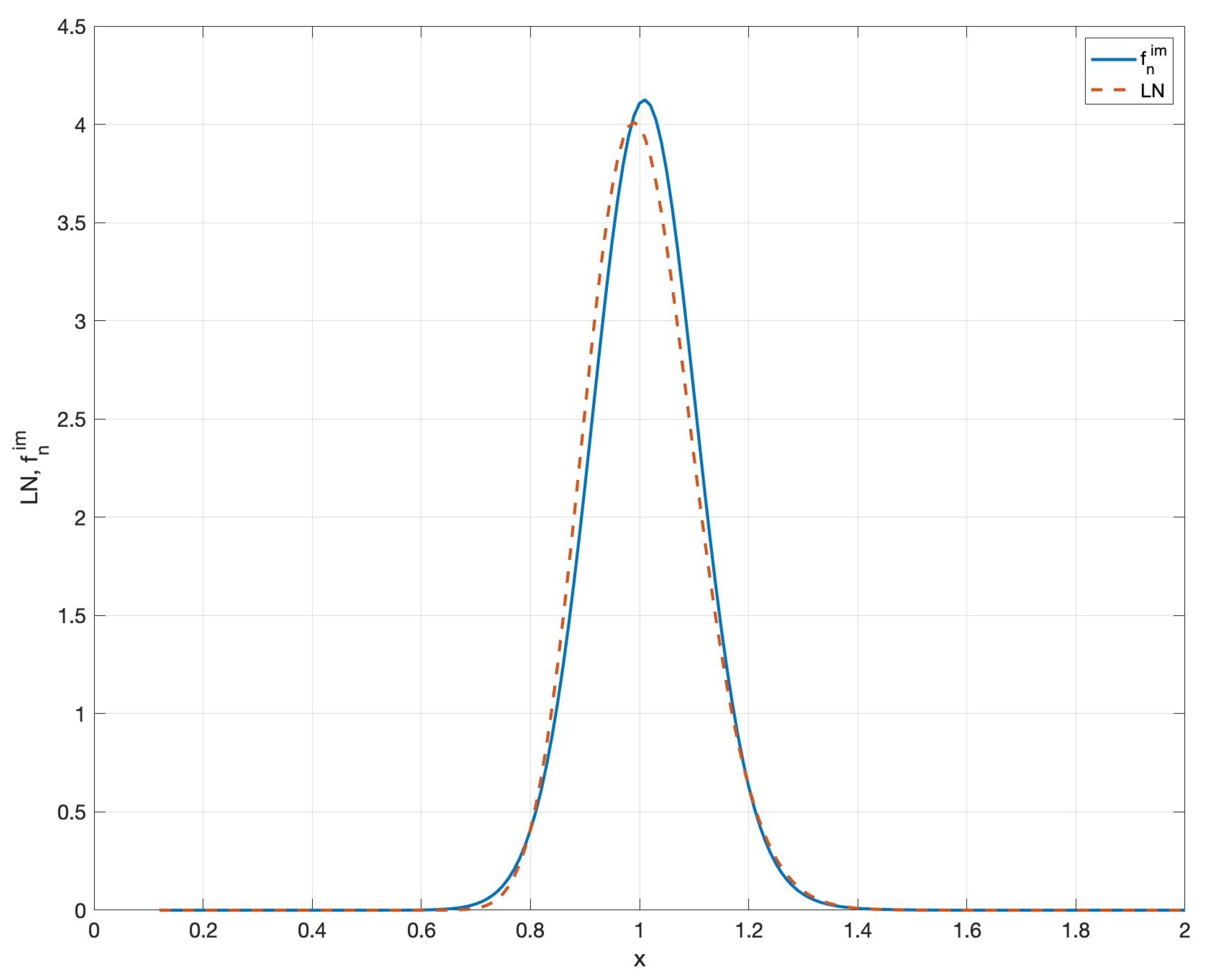
Example 1.

Out of pure curiosity, we wonder what $g_{hmax}$ is like once the sequence of moments has been assigned. Considering the various convergence criteria outlined above, $f_n^{im}$ can be considered a good approximation of $g_{hmax}$ as n assumes high values. And that is what we’re going to do, with an example.

Consider the standard lognormal $LN(0,{\sigma }^2)$ with density $LN$ and entropy $H\left[LN\right]={\displaystyle \frac{1}{2}}ln\left(2\pi e{\sigma }^2\right)\simeq -0.883646$ as $\sigma =0.1$, which guarantees ${lim}_{n\to \infty }H\left[f_n^{im}\right]=H\left[LN\right]$ is finite, according to Theorem 2 and [15], Thm. 7.

Table 1. $H\left[f_n^{im}\right]$ and difference $H\left[f_n^{im}\right]-H\left[LN\right]$, with $\sigma =0.1$, for an increasing number n of integer moments.

n	$\mathit{H}\left[{\mathit{f}}_{\mathit{n}}^{\mathit{im}}\right]$	$\mathit{H}\left[{\mathit{f}}_{\mathit{n}}^{\mathit{im}}\right]-\mathit{H}\left[\mathit{LN}\right]$
2	−0.876144	0.007501
4	−0.877783	0.006367
6	−0.881564	0.002084
8	−0.882228	0.001411
10	−0.882631	0.001015

shows the entropy $H\left[f_n^{im}\right]$ of the MaxEnt reconstruction $f_n^{im}$ with increasing n while Figure 2 displays $LN$ density and $f_n^{im}$. Here $n=10$ is the largest available value due to the numerical instability associated with the moment problem in the MaxEnt setup.

From Table 1, it can be seen that as n increases, the difference $H\left[f_n^{im}\right]-H\left[LN\right]$ tends to 0. Here, we observe that the entropy changes very little as we go from, say, six to ten moments. Since the entropy rapidly stabilizes as the number of moments increases, this suggests that the number of moments considered is high enough for the reconstructed density to be close to the estimated density $LN$. The example now illustrated provides an answer to the reasonable doubt outlined above: given that the moment problem for the lognormal density is indeterminate, one might expect that approximations based on a sequence of integer moments either fail to converge or converge to a different distribution with the same moments.

5. Final Remarks

At the end of this paper, we will briefly summarize the path taken and the main results obtained.

Due to the analytic form of the Shannon entropy functional and its concavity, there exists a (unique) maximum in correspondence of $g_{hmax}$; that is, this density has the maximum entropy in the class $C_{\infty }$ which contains all the distributions sharing the lognormal moment sequence with it. In the MaxEnt framework, $g_{hmax}$ represents the most entropy-representative element of the class $C_{\infty }$. Moreover, using the fact that the characterizing moments of the lognormal distribution are given by $\mathbb{E}[ln(X\left)\right]$ and $\mathbb{E}\left[{ln}^2\left(X\right)\right]$ and that they can be assimilated to fractional moments whose orders ${\alpha }_1$ and ${\alpha }_2$ tend to $0^{+}$, it has been proved by Theorem 2 that $g_{hmax}$ coincides with $LN$.

Now, considering the sequence of lognormal integer moments as constraints, we know that the MaxEnt approximation based on them, $f_n^{im}$, converges in entropy, and also almost everywhere, to $g_{hmax}$. Hence, by Theorem 3, $f_n^{im}$ converges almost everywhere to $LN=g_{hmax}$. Finally, it is possible to conclude that the lognormal distribution is characterized by the sequence of its integer moments. And this justifies the title of this paper.