1. Introduction
In recent years, consumers’ rising living standards have driven increased demand for fresh produce, making fresh food logistics a key component of modern logistics systems. However, the growing volume of fresh food deliveries has led to a significant increase in fuel consumption and carbon emissions, presenting major challenges to sustainable development [
1]. According to the “China Logistics Green Development Report” (2023), carbon emissions from the logistics sector account for 9% of the nation’s total emissions, with fresh food logistics consuming substantial energy due to strict temperature control requirements. Both the “China Road Transport Capacity Development Data White Paper” (2022) and the Mordor Intelligence report highlight that an increasing number of enterprises are adopting electric vehicles for distribution to reduce the environmental burden of logistics. Many companies have adopted electric vehicles for distribution to mitigate the environmental impact of logistics. However, the limited range and load capacity of electric vehicles make it difficult to fully replace conventional-fuel trucks. As a result, companies are increasingly implementing a hybrid delivery model that combines fuel-powered and electric vehicles. Against this backdrop, optimizing fleet composition and delivery routes while balancing corporate profitability, customer needs, and environmental sustainability has become a key research focus in the logistics field. Given the complexity of fresh food logistics, studying path optimization through the multi-objective optimization of segmented transshipment modes and heterogeneous fleet scheduling is essential for promoting the sustainable and efficient development of fresh food logistics.
Researchers have conducted extensive studies in green logistics path optimization and distribution time sensitivity to address the multifaceted challenges in fresh produce logistics. Li et al. [
2] incorporated CH
4 and N
2O emissions into the optimization framework for green logistics and used dynamic simulations to analyze the impact of vehicle load on energy consumption and emissions. Wu et al. [
3] considered road congestion at different times of the day, employing piecewise functions to model fluctuations in vehicle speeds, thereby improving the efficiency of fresh produce distribution while significantly reducing carbon emissions during transportation. Wen et al. [
4] developed an optimization model for multi-compartment electric vehicle deliveries, effectively mitigating peak-hour carbon emissions by addressing multi-temperature layer demands and congestion issues. The vehicle routing problem with time windows (VRP-TW) was first introduced by Dantzig and Ramser [
5] in 1959, and time sensitivity has since become a pivotal factor in optimizing fresh food logistics. Wu et al. [
6] proposed a multi-objective optimization model based on customer time sensitivity requirements, enhancing distribution flexibility and customer satisfaction. Amorim et al. [
7] introduced a planning model incorporating multiple time windows and vehicle constraints, enabling the efficient allocation of time windows to better align customer needs with logistics resources. He et al. [
8] designed a flexible time window framework that categorized client demands into “preferred time windows” and “acceptable time windows,” integrating incentive and penalty mechanisms to maintain the quality of perishable goods. Despite these advancements in environmental protection and time window design, most research has focused on single-vehicle models or single-stage path optimization, lacking a thorough exploration of coordinated fleet scheduling. Furthermore, some studies focus on electric vehicles as delivery carriers; however, their limited load capacity and driving range restrict delivery coverage and complicate their application in complex scenarios. Additionally, the joint optimization of time windows and carbon emissions remains scarce, with improvements in delivery efficiency often achieved at the expense of environmental sustainability.
In recent years, double-layer transportation has gained recognition as an efficient logistics model, with research increasingly focusing on optimizing transportation modes and vehicle types. Wang et al. [
9] proposed a double-layer segmented transportation model using ecological packaging as the transit subject. The first layer optimizes long-distance transport through the SST network, while the second layer employs NSGA-II to enhance terminal synchronized delivery. Yong et al. [
10] developed a collaborative multi-center hierarchical transport model that improves long-haul transport efficiency via resource sharing among logistics centers and optimizes end-delivery routes by incorporating temperature control constraints, thereby increasing delivery flexibility and precision. Peng et al. [
11] expanded the scope of delivery from intra-city segmented transport to multimodal transport involving road and rail, balancing transport time, costs, and cargo damage through a multi-objective optimization framework. The evolution of double-layer transportation networks has also diversified vehicle types [
12,
13], extending beyond conventional fuel-powered vehicles to include electric vehicles and drones. Xu et al. [
14] introduced a dual-layer model integrating drones and electric vehicles to address poor road accessibility in remote rural areas, achieving comprehensive logistics coverage. Yuan et al. [
15] proposed a two-stage model combining railway freight with trucking, improving the economic feasibility of long-distance transport by optimizing railway bidding strategies and refining truck-based short-distance delivery routes, thereby achieving synergistic gains in efficiency and profitability. Cheng et al. [
16] introduced a dual-tier delivery approach that integrates public transit with drones, where buses transport both goods and passengers and drones launch and land on bus rooftops to enable flexible delivery, significantly enhancing transport efficiency. While most studies focus on improving delivery efficiency and reducing empty load rates, research on environmental impacts and cargo loss remains limited. Additionally, in segmented transportation, many studies continue to rely on a single vehicle type without optimizing transport mode selection based on route characteristics. Even when heterogeneous vehicles are employed, their application primarily addresses issues like uneven vehicle utilization or topographical challenges rather than focusing on fresh food logistics as the central subject of study.
Researchers have developed various advanced heuristic methods to address complex path-planning challenges. Cui et al. [
17] employed an adaptive genetic algorithm (AGA) to dynamically adjust crossover and mutation probabilities based on individual fitness, thereby enhancing the algorithm’s local search capability. Li et al. [
18] optimized electric vehicle routing using a modified remove-and-replace genetic algorithm (RI-GA), which significantly reduced transportation costs. Ma et al. [
19] enhanced traditional ant colony algorithms by refining transition rules, introducing local and global pheromone update mechanisms, improving path search diversity, optimizing initial parameter settings and path construction, and ultimately improving solution quality. Fang et al. [
20] integrated the A* algorithm with the ant colony algorithm to develop a sophisticated hybrid algorithm that substantially accelerated the initial convergence speed. Zhang et al. [
21] proposed an improved hybrid ant colony optimization algorithm (HACO) for site selection and path optimization in two-stage cold chain logistics. By dynamically balancing determinism and randomness in node selection through adaptive probabilities, this algorithm enhanced exploratory capabilities during stagnation phases while optimizing pheromone updates to strengthen the identification of optimal paths. Fathollahi-Fard et al. [
22] introduced an advanced adaptive large-neighborhood search algorithm, incorporating linear relaxation and Bender’s decomposition techniques to refine the initial solution construction and search strategies. This method also integrates Tabu search and simulated annealing to improve neighborhood search efficiency and solution quality. Despite these significant advancements in path optimization, certain limitations persist. Some algorithms overly emphasize the initial solution optimization while neglecting the refinement of elite solutions. Furthermore, many algorithms exhibit limited multi-objective optimization capabilities. When combined with other strategies, they often encounter challenges related to complex parameter tuning and slow convergence rates.
This study addresses the limitations of existing research by focusing on the optimization of fresh produce distribution routes within a segmented transshipment framework. It proposes a series of improved methods and optimization models for the collaborative operation of fuel and electric vehicles. Specifically, the main contributions of this study are as follows:
(1) Building on the traditional single-stage, single-vehicle-type approach to fresh produce logistics, this study introduces a segmented transshipment model combined with the collaborative scheduling of multiple vehicle types. By integrating considerations of carbon emissions and distribution efficiency, the proposed approach enhances the applicability of logistics solutions in complex scenarios.
(2) A collaborative dispatching mechanism for heterogeneous fleets is designed based on delivery route characteristics, enabling the efficient allocation of tasks between fuel-powered and electric vehicles. This mechanism leverages the complementary advantages of both vehicle types to improve delivery efficiency, reduce resource waste, and enhance the robustness of the logistics system.
(3) To address multi-objective optimization requirements, an ant colony algorithm is employed, incorporating a system of large and small ants to enhance the initial exploration and strengthen high-quality path solutions in later stages. An adaptive volatility factor is introduced to reduce uncertainty in manual parameter adjustments, while an adaptive large-neighborhood search is integrated to improve the quality of elite solutions.
In this model, fuel-powered vehicles, with their superior endurance, handle long-distance transportation. As the delivery nears its final stages, the operation transitions to electric vehicles to improve the delivery efficiency and reduce carbon emissions, thereby meeting the environmental requirements of urban distribution. To address this issue, a mixed-integer nonlinear programming (MINLP) model is developed, incorporating factors such as transportation costs, time window constraints, cooling requirements, product damage, and carbon emissions. By precisely quantifying these costs, the model systematically optimizes route planning and vehicle scheduling. In recent years, several emerging technologies have been introduced to solve MINLP problems, including enhanced heuristic algorithms, reinforcement-learning-based intelligent optimization methods, Bender’s decomposition techniques, and hybrid path optimization approaches that integrate graph neural networks (GNNs) with deep reinforcement learning (DRL). These innovative methods offer more efficient and flexible solutions to path optimization challenges. This study employs the widely used ant colony algorithm to address the multi-objective requirements and complexities of fresh produce logistics route optimization, with targeted improvements implemented to overcome its inherent limitations.
2. Model
2.1. Description and Assumptions
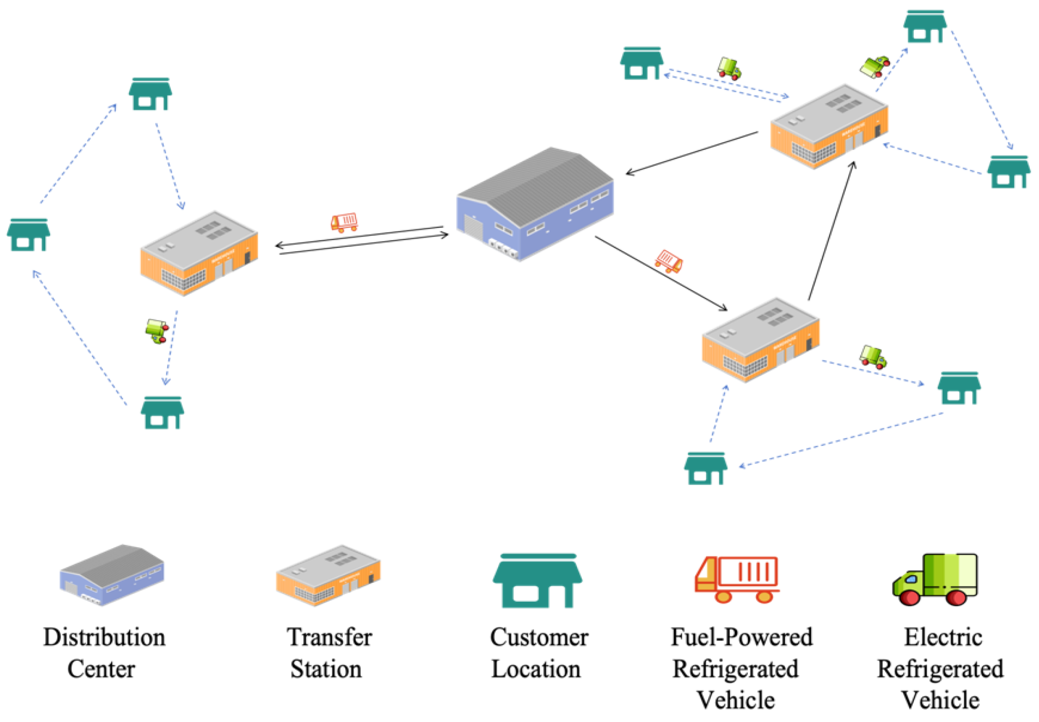
This study addresses the path optimization problem for fresh produce distribution using a heterogeneous fleet within a segmented transshipment mode. The distribution center operates a sufficient number of fuel-powered refrigerated vehicles to transport fresh goods to multiple transfer points. Subsequently, identical electric refrigerated vehicles, also available in sufficient quantities, handle the final delivery to customers from these transfer points (see
Figure 1). The model aims to minimize total distribution costs while considering environmental impact, customer requirements, and operational expenses. The characteristics of fuel-powered and electric vehicles during the different transportation phases are incorporated to optimize the fleet configuration and route planning. To ensure the rationality of the model, the following assumptions are made:
(1) Only a unidirectional fresh food distribution model from a single distribution center to multiple customer locations is considered;
(2) The distribution center is equipped with a certain number of fuel-powered vehicles of the same specification;
(3) The transshipment hubs are equipped with a certain number of electric vehicles of the same specification;
(4) Both the distribution center and the transshipment hubs are equipped with backup vehicles to handle uncontrollable factors, such as vehicle breakdowns;
(5) Each vehicle can serve multiple customer locations, but each customer location can only be served by one vehicle;
(6) Customer demand is known and does not exceed the maximum capacity of the vehicles;
(7) Fuel-powered vehicles start and end their routes at the distribution center, while electric vehicles start and end their routes at the transfer station;
(8) Roads connecting the distribution center, transfer stations, and customer locations are fully accessible;
(9) Electric vehicles leave the transfer station with a full charge and must return to recharge when the battery is insufficient;
(10) The locations of the transshipment hubs are assumed to be configurable at any point on the map.
2.2. Parameter Symbols and Variable Definitions
To ensure the completeness of the model construction, assumptions are made for the parameters and variables, as shown in
Table 1.
2.3. Objective Function
(1) Vehicle Transportation Costs
Vehicle transportation costs for the heterogeneous fleet include fixed and operating costs. Under the segmented transshipment mode, fuel-powered vehicles handle long-distance transportation, while electric vehicles are used for last-mile delivery. The operating costs for both vehicle types are calculated based on the distance traveled and energy consumption.
Fixed costs include vehicle acquisition, maintenance, and driver wages, which depend on the number of vehicles used. The formula for calculating fixed costs is:
where
CF and
CE denote the unit fixed costs for fuel-powered and electric vehicles, respectively.
Operating costs are directly related to distance traveled and energy consumption [
23]. In the segmented transshipment mode, the fuel consumption of fuel-powered vehicles depends on both distance and load, whereas the electricity consumption of electric vehicles remains relatively stable and primarily depends on the distance traveled. The formula for calculating operating costs is:
where
A and
B represent the fuel consumption and electricity consumption rates for fuel-powered and electric vehicles,
λ and
λ0 represent the fuel consumption per unit distance when fully loaded and empty, respectively,
γ represents the electricity consumption per unit distance for electric vehicles, and
Qin denotes the remaining cargo volume after leaving customer
i.
Thus, the total vehicle transportation costs are:
(2) Penalty Costs for Violating Time Window Constraints
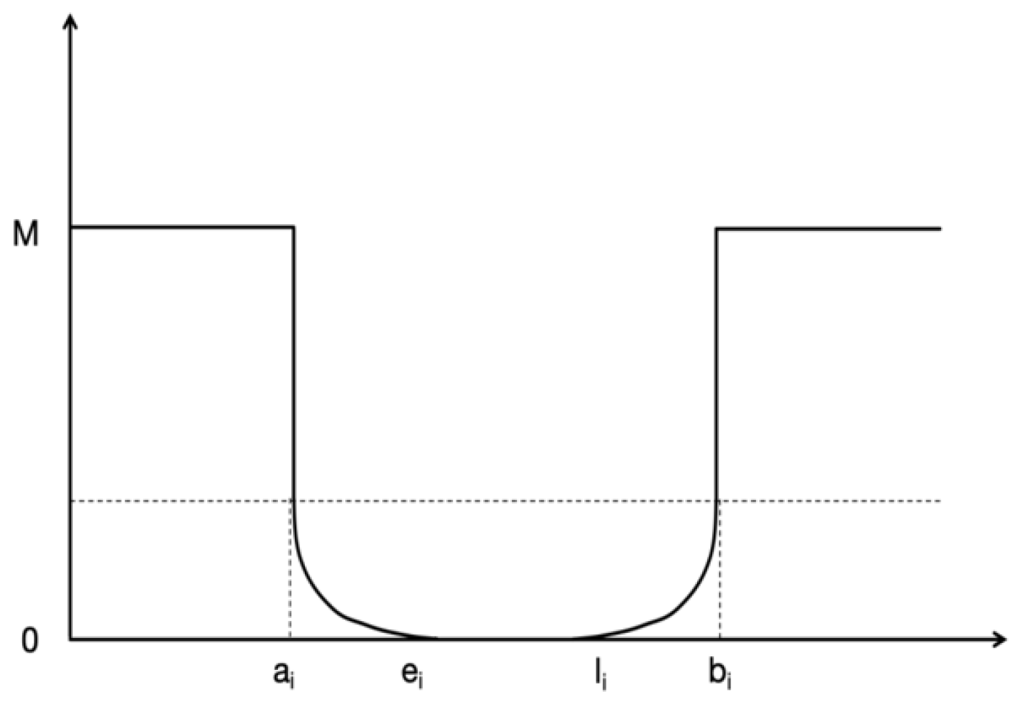
Due to the specific nature of fresh food distribution and the strict time requirements of customers, this study introduces a segmented penalty function to quantify the impact of time window deviations on costs (see
Figure 2). By adopting a segmented approach, the function more accurately reflects the influence of delivery timing on total costs [
24,
25].
In the figure, [
ei,
li] represents the ideal delivery time window acceptable to the customer, indicating the expected time frame for the arrival of goods. When the goods arrive within the intervals [
ai,
ei] or [
li,
bi], certain time window deviation costs are incurred but are still within the customer’s tolerance. However, if the goods arrive within the intervals [0,
ai] or [
bi, +∞], it is considered a severe violation of the scheduled time window, potentially leading to customer refusal and substantial fines. Therefore, route planning aims to avoid such situations to minimize time window penalty costs and maintain customer satisfaction. The time window penalty cost is calculated as follows:
(3) Refrigeration Costs
In the segmented transshipment mode, the heterogeneous fleet operates with different vehicle types, each utilizing a distinct refrigeration method: fuel-powered vehicles rely on engine-driven systems, while electric vehicles use electrically powered refrigeration. Due to differences in energy consumption, refrigeration costs must be calculated separately for each vehicle type.
For fuel-powered vehicles, refrigeration costs include those incurred during transportation and unloading. During transportation, refrigeration costs are proportional to driving time, and the system is turned off after the final delivery to conserve energy, as no cargo remains. During unloading, since fuel-powered vehicles stay at transshipment hubs for longer periods, the refrigeration system must work harder to maintain cargo freshness, making costs proportional to the unloading time. The refrigeration cost for fuel-powered vehicles is calculated as follows:
where
ω1 represents the refrigeration energy consumption per unit time during transportation, and
ω2 represents the energy consumption per unit time during unloading.
For electric vehicles, because end customers typically have smaller demands and shorter unloading times, refrigeration costs during unloading are negligible. Therefore, only transportation refrigeration costs, which are proportional to the driving time, need to be considered. The formula for calculating electric vehicle refrigeration costs is:
where
ω3 represents the refrigeration energy consumption per unit of time during transportation for electric vehicles.
In conclusion, the total refrigeration cost is:
(4) Cargo Loss Costs
Fresh products are highly sensitive to environmental conditions during transportation and unloading, and any changes in external conditions may lead to product loss. Considering the characteristics of the heterogeneous fleet, this study categorizes cargo loss costs into three parts: losses during the fuel-powered vehicle distribution phase, losses during the electric vehicle distribution phase, and potential damage from collisions throughout the entire transportation process.
For fuel-powered vehicles, cargo loss primarily includes freshness deterioration caused by respiration and losses due to temperature fluctuations during unloading. As fresh products are transported, their quality gradually decreases over time due to respiration, with the effect worsening as the transportation time increases. Additionally, since fuel-powered vehicles spend extended time at transshipment hubs, the temperature difference during unloading further exacerbates product loss. The formula for calculating cargo loss during this phase is:
where
P represents the unit value of fresh products,
qi represents the demand at customer point
i, and
ε represents the spoilage rate of fresh products at different stages.
For electric vehicles, cargo loss mainly depends on the degree of product degradation over time. As the transportation time increases, the quality of fresh products declines gradually. However, due to the higher unloading efficiency of electric vehicles, losses during unloading are negligible. The formula for calculating cargo loss in this phase is:
During loading and transportation, fresh products may also suffer damage from collisions or other physical impacts. The cost of such damage is calculated as:
In summary, the total cargo loss cost is:
(5) Carbon Emission Costs
Carbon emissions from fresh food distribution primarily result from vehicle operation and refrigeration systems. Given the use of a heterogeneous fleet in the segmented transshipment mode, this study calculates carbon emissions separately for fuel-powered and electric vehicles to highlight their differences.
For fuel-powered vehicles, carbon emissions originate from fuel consumption during transportation and the operation of the refrigeration system. Transportation emissions are closely related to the distance traveled and load weight, with fuel consumption and emissions increasing as both distance and load grow. The refrigeration system operates during both transportation and unloading to maintain cargo temperature, making its emissions proportional to the transport and unloading times. The formula for calculating the carbon emission cost of fuel-powered vehicles is:
where
Ctax represents the carbon tax, and ρ represents the emission factor at each stage.
Electric vehicles, although not directly producing exhaust emissions, generate indirect carbon emissions due to their reliance on electricity from the power grid. The carbon emissions of electric vehicles are proportional to mileage, with minimal impact from the load. The operation of the refrigeration system in electric vehicles is similar to that of fuel-powered vehicles. However, due to shorter unloading times, the refrigeration energy consumption and resulting carbon emissions during unloading are negligible. The formula for calculating the carbon emission cost of electric vehicles is:
Thus, the total carbon emission cost is:
2.4. Model Formulation
Equation (15) represents the objective function, which aims to minimize the total distribution costs of a heterogeneous fleet under the segmented transshipment mode. Equations (16) and (17) set the maximum load capacity constraints for fuel-powered and electric vehicles, respectively. Equations (18) and (19) ensure that each node is serviced exactly once. Equation (20) specifies that the starting and ending points for fuel-powered vehicles are at the distribution center, while Equation (21) defines the starting and ending points for electric vehicles at the segmented transfer stations. Equations (22) and (23) ensure that a vehicle departs from a node after arriving at that node. Equation (24) ensures that electric vehicles depart from the transfer stations fully charged. Finally, Equations (25)–(27) provide additional constraints.
3. Algorithm Design
To solve the path optimization problem for a heterogeneous fleet in the segmented connection mode, the k-means++ clustering algorithm is first employed to determine the locations of connection transfer stations, effectively partition delivery areas, and optimize the connection of each transportation segment. The delivery route of the heterogeneous fleet is subsequently refined using an improved ant colony algorithm (IAMACO). Given the specific characteristics of the research problem and the inherent limitations of the ant colony algorithm, several enhancements are made as follows:
(1) Designing heuristic information for several objectives: The conventional ant colony optimization (ACO) algorithm primarily focuses on single-objective optimization, making it challenging to attain an efficient balance among delivery costs, time window penalty costs, and carbon emission targets [
26,
27]. This study develops a multi-objective unified heuristic information formula and incorporates a dynamic weighting mechanism to modulate the significance of each objective based on specific requirements. This enhancement allows the method to concurrently evaluate many objectives in the path-planning process, increasing its relevance and utility in multi-objective optimization contexts.
(2) Introducing the Max–Min Ant System (MMAS): The ACO faces challenges such as excessive pheromone accumulation, which leads to local optima, or excessive volatilization, which reduces the convergence efficiency. To address these issues, this study integrates upper and lower pheromone limits into the algorithm to prevent the unlimited accumulation or complete depletion of pheromones. This improvement enhances the algorithm’s initial exploration capability and its ability to reinforce high-quality pathways in later stages, significantly improving the global search efficiency and solution quality.
(3) Designing an adaptive volatilization factor: The static volatilization factor in the ACO lacks flexibility, often resulting in excessive pheromone accumulation that traps the algorithm in local optima or rapid decay that causes the loss of valuable path information. This study introduces an adaptive volatilization factor that dynamically adjusts the intensity based on the disparity between the current solution and the global best solution. When the current solution approaches the optimum, volatilization is reduced to strengthen high-quality paths; conversely, when the solution deviates from the optimum, volatilization is increased to enhance global search capabilities. This improvement significantly enhances the algorithm’s flexibility and optimization performance.
(4) ALNS enhances the quality of elite solutions: In the later stages, the ACO heavily relies on elite solutions, making it prone to local optima due to a lack of dynamic optimization. To address this limitation, this study introduces ALNS, which enhances the quality of elite solutions through a destruction and reconstruction mechanism. Simulated annealing is incorporated to accept suboptimal solutions, thereby increasing the solution diversity [
28]. This improvement significantly enhances the algorithm’s global search capability and is particularly well suited for solving complex multi-stage optimization problems.
Overall, these improvements enable the ant colony algorithm to demonstrate greater adaptability and improved solution efficiency in addressing complex path optimization problems.
3.1. k-Means++ Clustering Algorithm
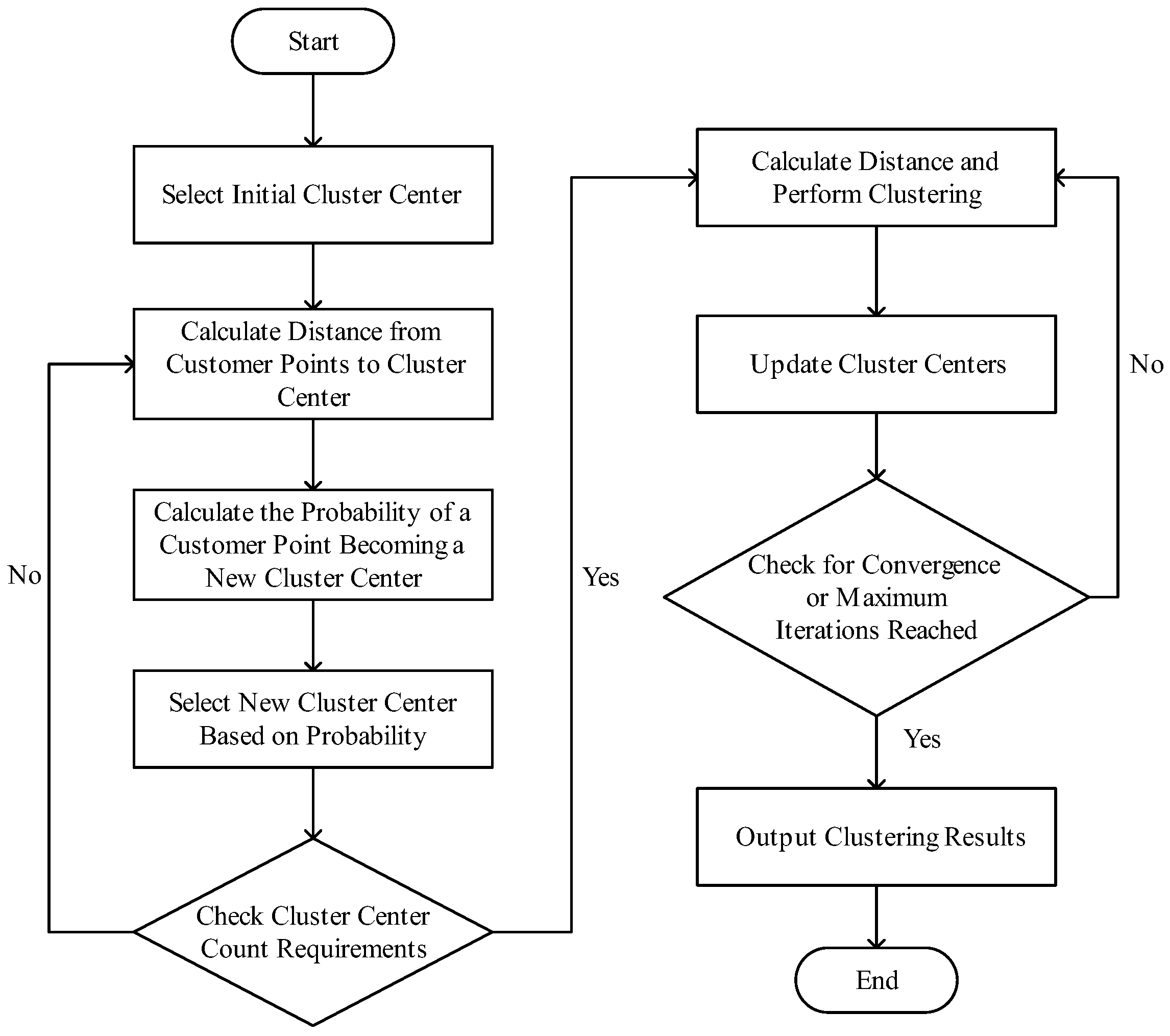
To determine transshipment hub locations more effectively, this study employs the k-means++ clustering algorithm (
Figure 3). The traditional k-means algorithm suffers from slow convergence and instability due to the random selection of initial cluster centers. K-means++ improves both the quality and stability of clustering by optimizing the choice of initial cluster centers, making it particularly suitable for complex delivery scenarios involving heterogeneous fleets under a segmented transshipment mode [
29]. The algorithm consists of the following steps:
Step 1: Initialization. A random customer point is selected from the dataset as the first cluster center
c1.
Step 2: Selecting subsequent cluster centers.
Step 2.1: Distance calculation. For each customer point x, the squared distance to the nearest selected cluster center
D(
x)
2 is computed.
Step 2.2: Probability calculation. Using
D(
x)
2 as the weight, the probability
p(
x) for each point to be chosen as the next cluster center is calculated.
Step 2.3: Selecting new cluster centers. Based on p(x), a new customer point is randomly selected as the next cluster center.
Step 2.4: Repeat selection. Steps 2.1 to 2.3 are repeated until k cluster centers are selected.
Step 3: Standard k-means clustering.
Step 3.1: Assigning data points. Each customer point x is assigned to the cluster corresponding to the nearest cluster center.
Step 3.2: Update cluster centroids. The new cluster center for each cluster is computed as the average of all data points within that cluster.
Step 3.3: Termination condition. The algorithm terminates when the cluster centers stop changing or when the maximum number of iterations is reached, and the final clustering results are produced.
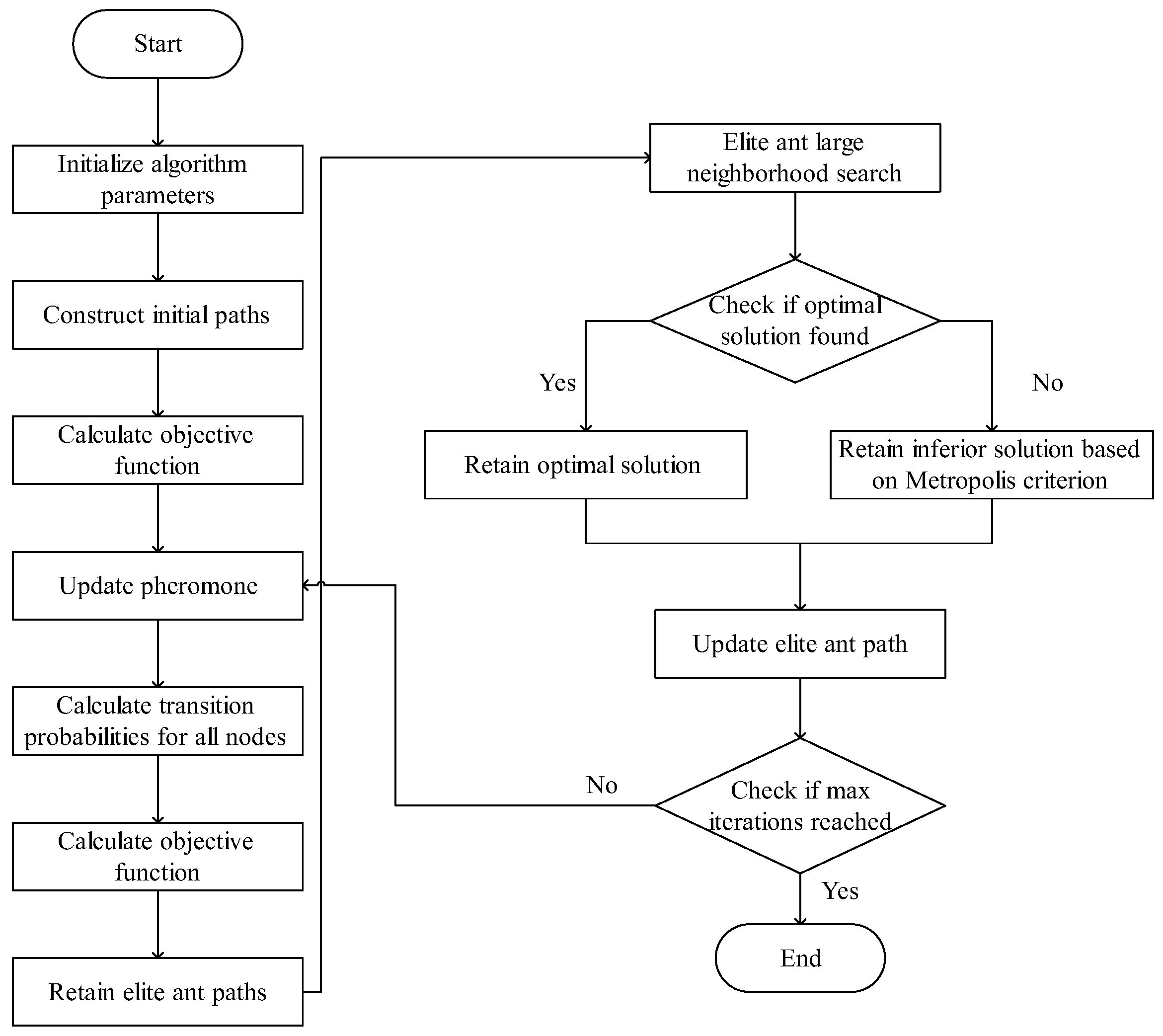
3.2. Improved Adaptive Multi-Objective Ant Colony Algorithm
Step 1: Initialization. Key parameters such as the number of ants, the maximum number of iterations, the initial pheromone concentration, and the evaporation coefficient are set to establish the optimal initial conditions. Based on these parameters, the initial set of paths for the ants is generated.
Step 2: Objective function calculation. After each ant completes its path construction, the value of the objective function is calculated for its path. The objective function integrates the total path cost, time window violation cost, and carbon emission cost to achieve multi-objective optimization. The specific formula is as follows:
Step 3: Pheromone update. In each iteration, the pheromone levels on all paths are updated to guide the ants toward more optimal routes in subsequent iterations. To effectively control pheromone variation, the Max–Min Ant System is applied, setting upper
τmax and lower
τmin bounds for pheromone levels. This prevents the unlimited accumulation or depletion of pheromones, thereby reducing the risk of convergence to a local optimum. The formula for pheromone update is:
Furthermore, to balance exploration and exploitation capabilities, an adaptive evaporation factor strategy is employed, which dynamically adjusts the evaporation factor based on the gap between the current solution and the global optimal solution. The specific formula is as follows:
Step 4: Path selection completion. In each iteration, each ant selects the next node by calculating the transition probability, continuing this process until all nodes are visited, thereby forming a complete path. The transition probability is determined by both the pheromone concentration and heuristic information and is calculated using the following formula:
Step 5: Elite path retention and large-neighborhood search. In each iteration, the current best elite solution is retained, and a large-neighborhood search is performed to expand the solution space, thereby enhancing the global optimization capability.
Step 6: Solution quality evaluation. After destroying and reconstructing the elite solution, the quality of the new solution is evaluated. If the new solution is better than the current elite solution, the elite solution is updated; otherwise, the original elite solution is kept and the Metropolis criterion is used to determine whether to accept the inferior solution, thereby increasing the likelihood of escaping local optima.
Step 7: Elite ant path update. Regardless of whether a better solution is found, the elite path is updated to ensure continuity in pheromone transmission.
Step 8: Termination assessment. If the maximum number of iterations is reached, the process is terminated and the optimal solution is output; otherwise, iteration continues.
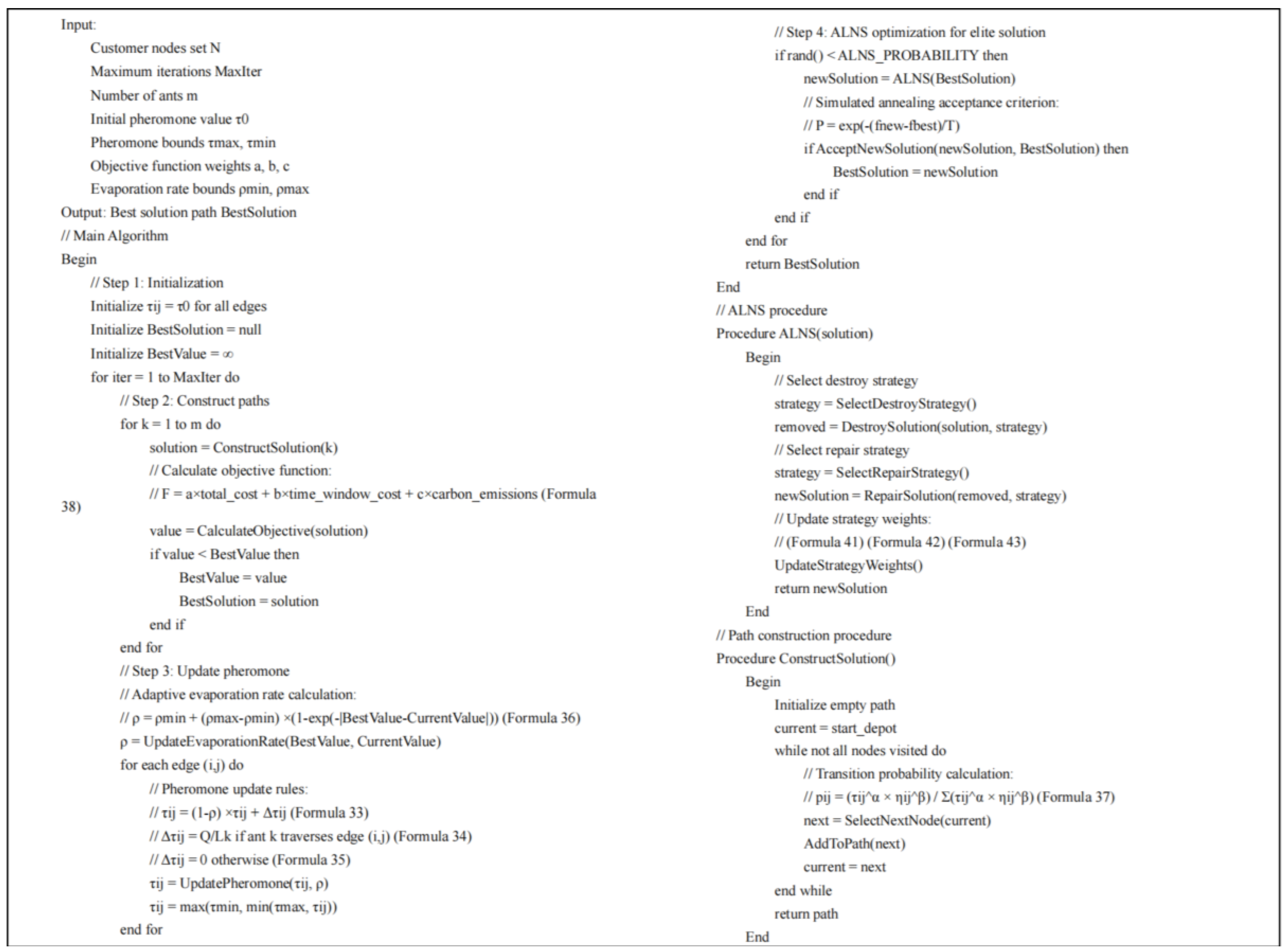
The algorithm flow is shown in
Figure 4. To provide a more intuitive description of the implementation steps of the improved ant colony algorithm, the corresponding pseudocode is presented in
Figure 5.
3.3. ALNS Strategies for Optimizing Elite Solutions
Adaptive large-neighborhood search (ALNS) is a heuristic algorithm widely applied to complex combinatorial optimization problems [
30]. Its core concept lies in adaptively exploring optimal solutions within the neighborhood of the current solution through various destruction and reconstruction strategies. Unlike a traditional large-neighborhood search, ALNS incorporates an adaptive mechanism that dynamically adjusts the weight of each strategy based on its performance during the algorithm’s execution, achieving a balanced trade-off between global search and local optimization. This section details its application in enhancing elite solutions through the design of destruction strategies, reconstruction strategies, and acceptance and adaptation criteria.
3.3.1. Destruction Strategy
The destruction strategy consists of three approaches: single-point destruction, multi-point destruction, and correlation-based destruction.
(1) Single-point destruction: A customer point i is randomly selected and removed from the current solution. This strategy introduces minor local adjustments to the solution, helping prevent the algorithm from becoming trapped in local optima at an early stage. It also provides more exploration opportunities for subsequent path adjustments and optimization.
(2) Multi-point destruction:
M customer points are randomly selected for removal, where
M is determined by Equation (38). This approach significantly alters the overall structure of the solution, breaking local constraints and enhancing the exploratory capability of the search.
where randi(
m1,
m2) represents a random number selected within the range of
m1 and
m2, and
N denotes the total number of customer points.
(3) Correlation-based destruction: A customer point
i is randomly selected, and its correlation
D with other customer points is calculated. The customer point with the highest correlation is then removed. This process is repeated until
M customer points are removed. The correlation
D is calculated as follows:
Here, dij represents the normalized distance between customer points i and j, while vij indicates whether customer points i and j belong to the same delivery route. If they do, vij = 1; otherwise, vij = 0.
3.3.2. Reconstruction Strategy
The reconstruction strategy is divided into two methods: time window cost reconstruction and maximum difference reconstruction.
(1) Time window cost reconstruction: When reinserting a removed customer point, its time window compliance and cost increment across all potential insertion positions are evaluated. Priority is given to the position that meets the time window requirement while minimizing the cost increment, thereby minimizing the overall cost increment of the solution.
(2) Maximum difference reconstruction: For each removed customer point i, its optimal insertion position
p1 and second-best position
p2 within the current solution are determined using the total path distance increment
R(p). Then, the objective function difference, Δ
R, is calculated, which represents the additional path length incurred by choosing the second-best position
p2 over the optimal position
p1. The customer point with the largest Δ
R is prioritized for insertion at the optimal position
p1 to minimize the overall path length.
3.3.3. Establishment of Acceptance Criteria
The simulated annealing criterion is adopted as the acceptance rule for new solutions, aiming to balance exploration and exploitation. By setting an initial temperature and gradually reducing it, the probability of accepting inferior solutions can be controlled. At higher temperatures, even suboptimal solutions are likely to be accepted, which helps prevent the algorithm from converging prematurely to local optima.
3.3.4. Establishment of Adaptive Criteria
An adaptive adjustment mechanism is introduced to dynamically optimize the selection of removal and insertion strategies by adjusting the weights of each strategy according to their actual performance during algorithm execution, thereby enhancing the algorithm’s efficiency and solution quality. In the algorithm’s initial phase, the weights of both the removal and insertion operators are assigned a value of 1, guaranteeing an equal probability of selection for each operator at the onset of the optimization process. This preliminary weight configuration can augment the algorithm’s exploratory characteristics and offer varied search trajectories for future optimization. The weights of the removal and insertion operators are dynamically modified after each iteration according to their performance. The formula for updating weights is as follows:
In this context, fr and fi represent the weights of the removal algorithm and the insertion operator, respectively, whereas σ denotes the weight for rewards and penalties. m is a binary control variable. When an operator is chosen, m = 1, and its weight is modified; otherwise, m = 0, and the weight remains constant. η is a weight coefficient utilized to regulate the extent of dependency of the operator weight on historical and current performance. This value is established at 0.8 to equilibrate the stability and flexibility of weight adjustment in this study. This number has been corroborated by numerous studies and can efficiently equilibrate the sensitivity and stability of weight updates.
In each iteration, the algorithm selects between the removal and insertion of operators using a roulette mechanism, with the selection probability proportional to the current operator’s weight. The chance of selection is computed as follows:
where
Pr(t) and
Pi(t) denote the selection probabilities of the removal and insertion operators, respectively.
4. Experimental Simulation and Results Analysis
To validate the proposed model and algorithm, two types of experiments were conducted. The first set of experiments used the Solomon standard dataset to evaluate the performance of the improved ant colony optimization algorithm (IAMACO), focusing on optimal fitness, path distance corresponding to optimal fitness, and algorithm stability. By comparing IAMACO with the classical ant colony algorithm and other optimization techniques, the superiority of IAMACO in solving complex path optimization problems was verified. The second set of experiments utilized real operational data from a fresh food logistics company to evaluate the effectiveness of the segmented transshipment model. Key indicators, including the total distribution cost, refrigeration cost, cargo loss cost, and carbon emissions, were analyzed to validate the model’s applicability and advantages in fresh food distribution scenarios.
This study further enumerates the decision variables and constraints to provide a clearer understanding of the model’s scale and complexity. The proposed model includes six integer variables, three binary variables, four continuous variables, and twelve constraints. These variables and constraints reflect the high-dimensional complexity of the problem and the challenges in achieving an optimal solution. To simplify the solution process, certain nonlinear objective functions are approximated as piecewise linear functions. This approach significantly reduces the computational overhead, enabling the model to produce feasible solutions within a reasonable timeframe. Although this approximation may introduce some variance, potentially affecting the accuracy of the specific objectives, the optimization in this study prioritizes overall trends and global optimization results rather than the precision of individual solutions. Therefore, this approximation method is considered both reasonable and acceptable for practical applications.
Additionally, all experiments were implemented in MATLAB (version 2024b) on a MacOS M2 system.
4.1. Standard Dataset Simulation and Results Analysis
To evaluate the performance of the improved ant colony optimization algorithm (IAMACO) in optimizing delivery routes for heterogeneous fleets under segmented transshipment mode, the C1, R1, and RC1 datasets from the Solomon standard dataset were selected for testing. The C-type dataset features a dense node distribution, suitable for high-density delivery scenarios; the R-type dataset has dispersed nodes, simulating long-distance delivery challenges; and the RC-type dataset presents a balanced node distribution, ideal for optimizing mixed delivery routes. These datasets represent various logistics scenarios, providing a comprehensive evaluation of the algorithm’s adaptability and robustness in diverse environments. Each dataset contains 100 customer nodes, and the algorithm’s performance was evaluated using the optimal fitness as the objective function. The optimal fitness was obtained by weighting and summing the vehicle count, travel distance, and time window violation costs. Considering these factors comprehensively, the optimal fitness effectively reflects the overall logistics cost, thereby verifying the enhanced ant colony algorithm’s capability in solving complex path optimization problems.
The algorithm parameters were set as follows: adaptive adjustment coefficient for operator weight η = 0.5, iteration limit for ant colony algorithm Ant_max = 500, number of ants m = 30, pheromone concentration coefficient α = 2, heuristic information coefficient β = 8, total cost weight a = 0.5, time window violation weight b = 0.3, carbon emission weight c = 0.2, pheromone update constant Q = 100, maximum evaporation factor ρmax = 0.99, and minimum evaporation factor ρmin = 2.
4.1.1. Optimal Fitness Evaluation
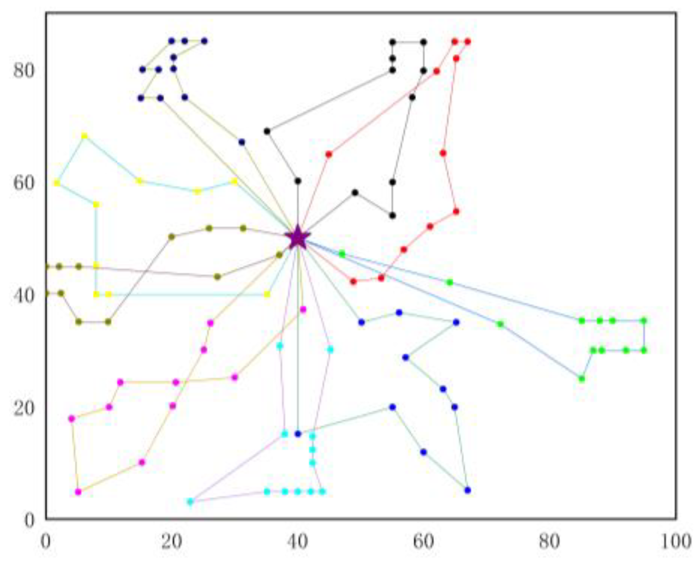
The evaluation was conducted using three datasets: C1, R1, and RC1. For simplicity and to represent the overall trend of each dataset, only one representative path map from each dataset is presented.
Figure 6,
Figure 7 and
Figure 8 depict the optimal path results based on the optimal fitness objective for the C102, R104, and RC104 datasets, respectively.
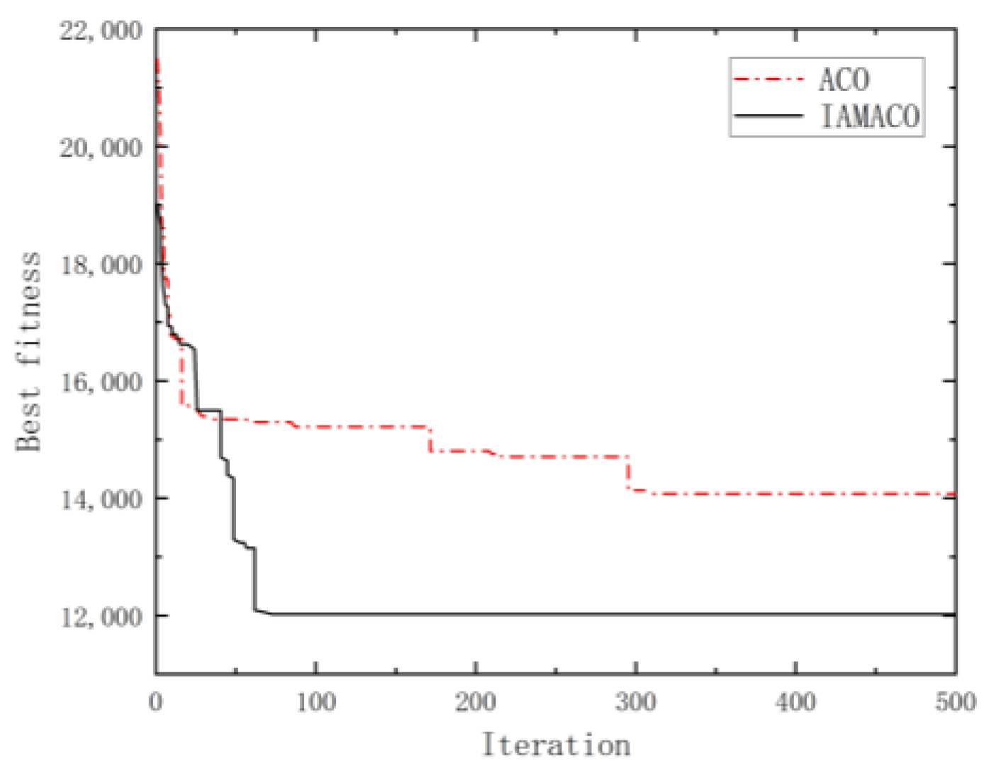
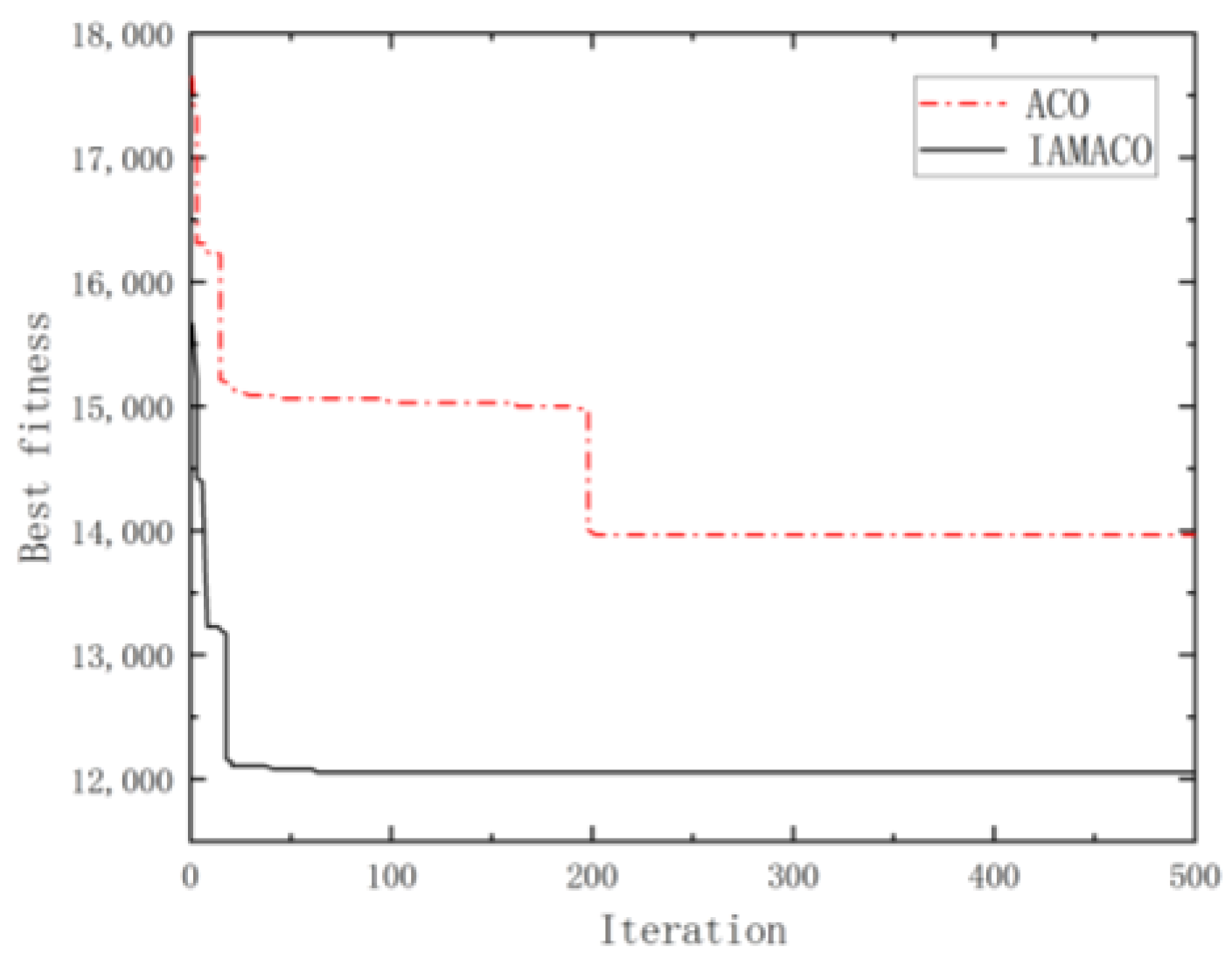
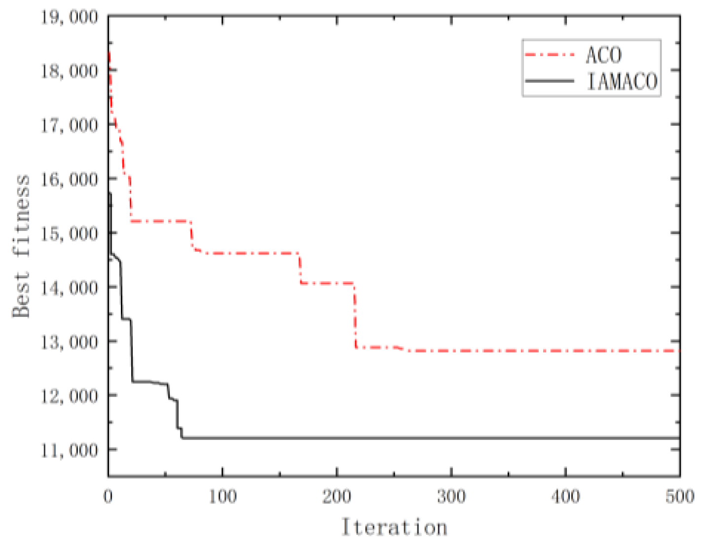
Figure 9,
Figure 10 and
Figure 11 demonstrate the iterative process of the ant colony algorithm before and after the improvements on the C102, R104, and RC104 datasets.
The path maps in
Figure 6,
Figure 7 and
Figure 8 demonstrate that the improved ant colony algorithm exhibited superior path-planning capabilities across the various delivery scenarios. In the high-density, long-distance, and mixed delivery contexts, the improved algorithm generated more compact and rational routes, effectively reducing detours and redundant paths and improving transportation efficiency.
Figure 9,
Figure 10 and
Figure 11 further illustrate that the improved algorithm achieved a faster convergence rate. During the initial iteration phase, the objective function value dropped rapidly, and the entire convergence process remained stable, indicating significant improvements in global search capability and solution stability. This enabled the algorithm to find the optimal solution more efficiently.
4.1.2. Driving Distance Test Based on Optimal Fitness
Although the optimal fitness provides a comprehensive measure of the algorithm’s overall performance in minimizing total costs, driving distance remains a key indicator in path planning, particularly for logistics distribution and carbon emissions. Under optimal fitness conditions, a shorter driving distance directly translates to reduced fuel or electricity consumption, effectively reducing the emission of greenhouse gases such as carbon dioxide. Therefore, analyzing the driving distance under optimal fitness conditions offers a more thorough evaluation of the algorithm’s effectiveness in optimizing path planning. In this study, both the shortest path distance and the average path distance were derived from 50 independent tests to effectively evaluate the algorithm’s overall performance under varying operating conditions.
The comparative analysis presented in
Table 2 indicates that the enhanced ant colony algorithm demonstrated substantial optimization impacts on the C1, R1, and RC1 datasets. The IAMACO method surpassed the conventional ant colony algorithm in evaluating the shortest and average path distance. This outcome indicates that the enhanced elite destruction and reconstruction technique augments the algorithm’s problem-solving capacity, enhancing the overall logistics and distribution efficiency. While certain enhanced ant colony algorithms exhibit a marginally elevated average running time compared to conventional ant colony algorithms, this is attributable to an augmentation in algorithmic complexity aimed at a more profound exploration of the solution space to identify superior solutions, thereby enhancing the overall quality of comprehension.
Moreover, path optimization enhances delivery efficiency while substantially decreasing vehicle fuel consumption and carbon emissions. Reduced driving distances directly diminishes carbon emissions per delivery, thus facilitating the establishment of an environmentally sustainable and efficient logistics system. This outcome demonstrates that the enhanced elite demolition and reconstruction technique exhibits superior algorithmic performance and significant application value in advancing green logistics development.
This study evaluated the reliability and stability of the enhanced ant colony algorithm through 50 independent tests, providing a more comprehensive performance analysis. The success rate quantifies the algorithm’s ability to identify high-quality solutions across multiple iterations, defined as the ratio of instances where the critical value solution is achieved to the total number of iterations. Stability is quantified using the standard deviation of the experimental results. A lower standard deviation indicates reduced solution volatility under varying operating conditions, thereby demonstrating greater robustness. The specific test results are presented in
Table 3.
In terms of reliability, the improved ant colony algorithm achieved a 100% success rate on the C1, R1, and RC1 datasets, significantly outperforming the standard ant colony algorithm. This demonstrates its strong global search capabilities, allowing the algorithm to repeatedly find optimal solutions. In terms of stability, the improved algorithm exhibited a significantly lower standard deviation compared to the standard algorithm, indicating more stable solution quality and enhanced robustness.
This study conducted a comparative examination of the improved ant colony algorithm (IAMACO) against the whale optimization algorithm (WOA), grey wolf optimization algorithm (GWO), and hybrid firefly algorithm (HFA) to thoroughly assess its efficacy in addressing complicated challenges. These algorithms excel in path optimization and combinatorial optimization problems, possess diverse application scenarios, and hold significant research value. The whale optimization algorithm (WOA) emulates the bubble net feeding technique of humpback whales during predation, excelling in global search and local refinement, hence rendering it appropriate for nonlinear and intricate challenges [
31]. The grey wolf optimizer (GWO) algorithm emulates the hunting behavior of grey wolves, featuring a straightforward and efficient framework, and it is extensively applied in path optimization and multi-objective problems [
32,
33]. The hybrid firefly algorithm (HFA) integrates the firefly algorithm with various optimization techniques to enhance search capabilities and solution quality via a hybrid approach [
34]. The RC104 dataset was chosen as the test dataset due to its intricate node distribution, which can effectively assess the adaptability and performance of algorithms in challenging settings.
Table 4 shows that the IAMACO algorithm outperformed the classical algorithms in both the optimal and average solutions. Although IAMACO’s average iteration count was slightly higher than that of the GWO algorithm, it was still lower than the other algorithms, ensuring a rapid convergence rate. Moreover, IAMACO demonstrated excellent performance in terms of computational time, further proving its efficiency and applicability in practical scenarios.
In summary, the improved ant colony algorithm outperformed the standard ant colony algorithm and other classical optimization methods in terms of solution quality, reliability, stability, and computational efficiency. When addressing complex path optimization, IAMACO exhibits higher solution accuracy, convergence efficiency, enhanced global search capabilities, and rapid convergence characteristics, making it especially suitable for logistics path optimization with complex constraints.
4.2. Simulation and Results Analysis of the Real-World Case Study
This study employed actual operational data from a fresh food chain in Dalian, China, to validate the proposed model and algorithm through simulation analysis. The store offers a wide range of products, including fresh fruits, vegetables, meat, seafood, and dairy products, ensuring freshness and timely delivery. To maintain product quality, the chain has established its own cold chain logistics system, constructing an independent distribution network that delivers goods directly from the distribution center to retail outlets. This setup avoids potential delays and quality risks associated with third-party logistics. Using this store’s logistics data, the model and algorithm were validated for their effectiveness in real-world fresh food distribution scenarios [
35].
Table 5 presents the detailed information for each store. The additional parameters of the model are as follows: The fixed cost of the fuel-powered vehicle
CF is RMB 180, and the fixed cost of the electric vehicle
CE is RMB 150. The speed of the fuel-powered vehicle
vF is 60 km/h, while the speed of the electric vehicle
vE is 60 km/h. The maximum load of the fuel-powered vehicle
QF is 2800 kg, and the maximum load of the electric vehicle
QE is 1500 kg. The unit fuel cost
A is RMB 8.02 per liter, and the unit electricity cost
B is RMB 1.5 per kWh. The fuel consumption per unit distance of the fuel-powered vehicle
λ is 1.5 L per km, and the electricity consumption per unit distance of the electric vehicle
γ is 18 kWh per km. The time window penalty factor
u is 1.5. The energy consumption per unit cooling time
ω1,
ω2, and
ω3 is 6.416 L/h, 0.75 L/h, and 1.2 kWh/h, respectively. The unit value of fresh produce
P is 10. The spoilage rates of fresh produce
ε1,
ε2,
ε3, and
ε4 are 0.0008, 0.0009, 0.0008, and 0.0009, respectively. The carbon tax
Ctax is RMB 0.15 per kg, and the carbon emission factor
ρ is 2.64.
A fleet delivery route plan was generated through 100 iterations of the enhanced ant colony algorithm. To ensure the reliability of the plan, 20 independent tests were conducted, and the best-performing route was selected. Due to the characteristics of heuristic algorithms, the obtained solution represents a relatively optimal result, achieving efficient multi-objective optimization within a reasonable computational time.
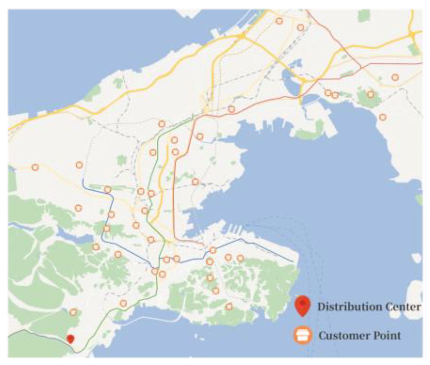
Figure 12 displays the layout of the distribution network, visually illustrating the geographical distribution of the distribution center and retail outlets, aiding in understanding the network’s coverage and the distance between outlets.
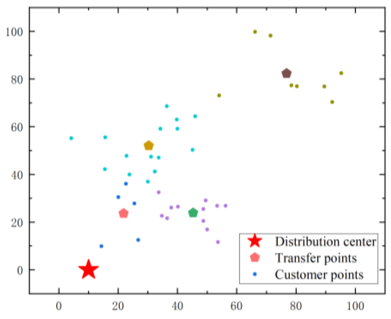
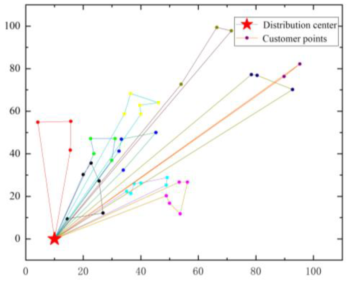
Figure 13 shows the clustering results of the outlets based on their geographical locations, providing a scientific foundation for subsequent route optimization. The optimal delivery routes under different modes are depicted in
Figure 14 and
Figure 15, with
Figure 15 further detailing the optimized routes and service order.
Upon comparing the data in
Table 6, the segmented connection model demonstrated substantial advantages across all metrics. The total distribution cost for the heterogeneous fleet integrated with this model was RMB 2373.13, representing a reduction of 22.13% compared to the single-fleet mode. This optimization benefit primarily arose from the endurance advantage of fuel-powered vehicles in long-distance transportation combined with the lower operating costs of electric vehicles in last-mile deliveries. In terms of time window penalty costs, the heterogeneous fleet incurred a penalty of RMB 49.50, which is 28.32% lower than that of the single-fleet mode. This indicates that electric vehicles offer greater flexibility in last-mile distribution, allowing them to meet delivery schedules more effectively and better fulfill customer expectations. Regarding carbon emissions, the heterogeneous fleet resulted in RMB 31.53 in carbon emission costs, which is 41.08% lower compared to the single-fleet mode. This illustrates that using electric vehicles for short-distance transport effectively reduces carbon emissions, enhancing the overall environmental sustainability of the distribution process. Finally, in terms of carbon emission costs, the heterogeneous fleet produced emissions valued at RMB 31.53, representing a 41.08% reduction compared to the single-fleet model. This result demonstrates that the application of electric vehicles in short-distance transportation significantly reduces carbon emissions, enhancing the overall environmental efficiency of transportation. Additionally, the segmented transshipment mode exhibits substantial environmental potential in urban delivery scenarios. By reducing greenhouse gas emissions, this mode effectively alleviates air pollution during urban distribution, improves urban environmental quality, and contributes to enhancing residents’ living standards. Furthermore, the significant reduction in carbon emissions under the segmented transshipment mode provides practical support for logistics companies in fulfilling their social responsibilities, aiding them in achieving a green transition while advancing energy conservation and emissions reduction.
Based on the analysis of vehicle usage in
Table 7, the number of electric vehicles significantly increased to fifteen in the segmented transshipment mode, primarily handling last-mile deliveries, while the number of fuel-powered vehicles decreased to three, mainly responsible for long-distance transportation. After completing their delivery tasks, electric vehicles return to the transfer point for recharging in preparation for the next round of deliveries. The integration of a recharging mechanism not only extends the operational time of electric vehicles and enhances their flexibility in last-mile distribution but also eliminates the need for additional vehicles due to range limitations. This optimization improves resource allocation and reduces overall operating costs.
In summary, the heterogeneous fleet integrated with the segmented transshipment mode outperformed the traditional single-fleet model in several key aspects, including total distribution cost, time window violation cost, and carbon emissions. These results not only validate its effectiveness in real-world fresh food distribution but also highlight its potential for optimizing cost control, improving delivery efficiency, and reducing environmental impact.
4.3. Sensitivity Analysis
4.3.1. Sensitivity Analysis of Energy Costs
This study developed three types of scenarios to assess the influence of fluctuations in energy costs on the model optimization outcomes: single-factor changes, two-factor changes, and extended scenarios. Single-factor change: This mainly assesses the independent variations in fuel or power costs and evaluates the influence of a singular variable on overall transportation expenses. Two-factor change: This examines the cumulative effect of concurrent modifications to fuel and electricity costs and evaluates the influence of overlapping energy prices on the model. This evaluates the model’s flexibility in a multifaceted real-world setting. A systematic analysis of these scenarios can reveal the model’s adaptability to fluctuations in energy prices and the adjustment characteristics of the route planning strategy.
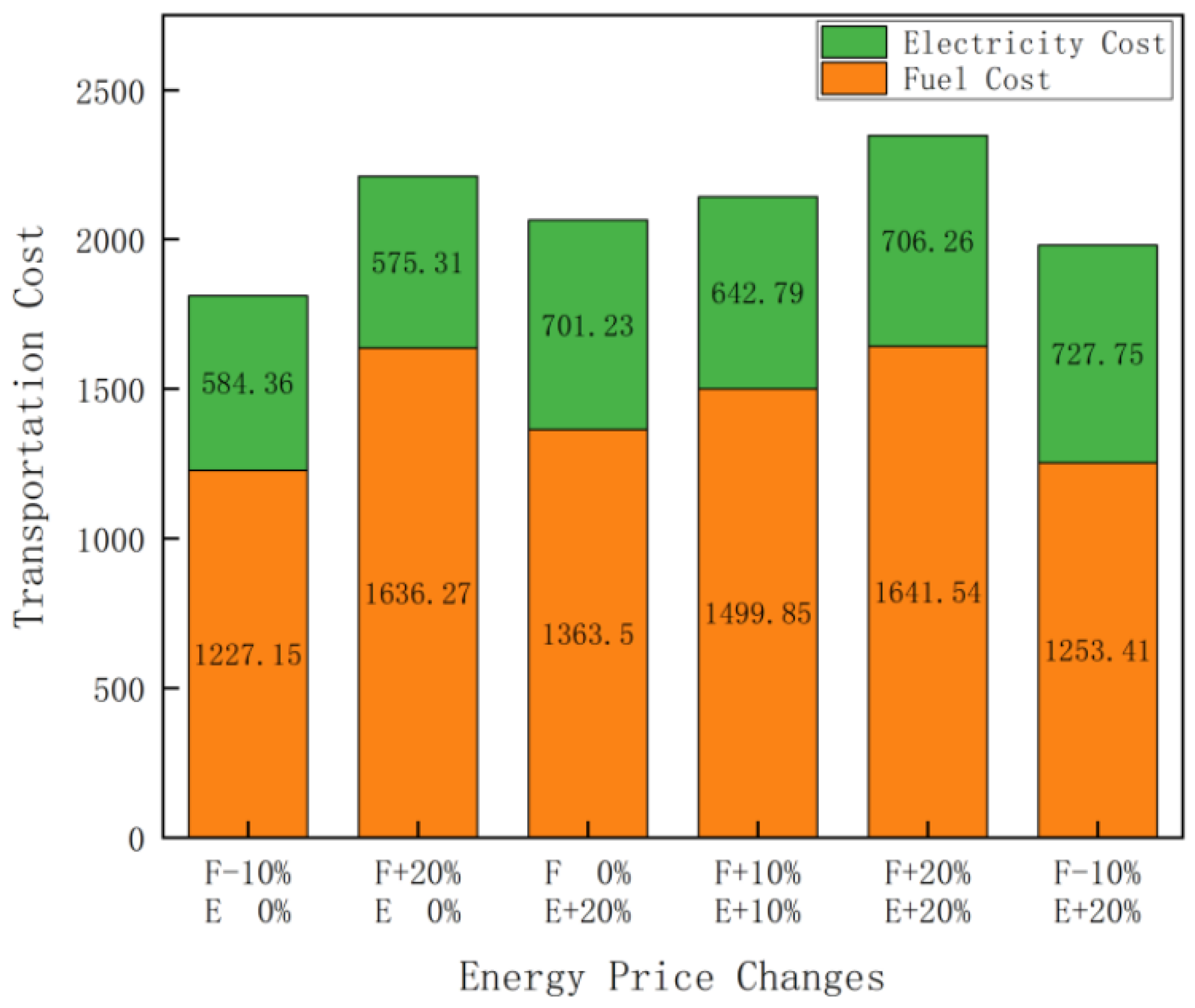
Figure 16 illustrates that fuel expenses exerted the most significant influence on the overall transportation costs, with fluctuations in fuel prices having a more pronounced impact than electricity expenses. A 10% decrease in fuel costs reduced the transportation costs from RMB 1947.86 to RMB 1811.51, a reduction of approximately 7%. Conversely, a 20% increase in fuel costs raised the total expenses to RMB 2211.58, representing an increase of about 13.5%. In comparison, variations in electricity costs had a much smaller impact. Even with a 20% increase in electricity rates, the total cost only rose from RMB 1947.86 to RMB 2064.73, reflecting an approximate increase of 6%. Moreover, when both fuel and electricity costs increased by 20%, the total cost rose sharply to RMB 2347.80, an increase of around 20.5%, underscoring the dominant role of fuel costs in the superposition effect. Thus, fuel cost fluctuations not only significantly affect total transportation costs but also play a key role in the combined effect of energy prices, making them a critical factor in optimizing transportation expenses.
Fluctuations in fuel costs also directly influence carbon emission levels. As fuel prices rise, the cost of using gasoline-powered vehicles increases, enhancing the economic advantages of electric vehicles. This shift results in more transportation tasks being allocated to electric vehicles, significantly reducing carbon emissions. Conversely, lower fuel prices may lead to increased use of gasoline-powered vehicles and, consequently, higher carbon emissions. Therefore, fuel costs are a pivotal factor not only in terms of transportation expense optimization but also in terms of environmental impact. Integrating the promotion of new energy vehicles with carbon emission cost considerations can effectively optimize transportation costs while advancing the goal of green logistics.
4.3.2. Sensitivity Analysis of Time Windows
Five scenarios were designed to evaluate the impact of time window variations on the model optimization: a base scenario, 10% reduction, 30% reduction, 10% relaxation, and 30% relaxation. A shorter time window simulates stricter delivery requirements, analyzing their effects on the total costs and time window violation costs. Conversely, a relaxed time window represents looser constraints and evaluates the improvements in optimization outcomes. This systematic analysis revealed the sensitivity of path planning and cost optimization to time window adjustments as well as the model’s adaptability.
Table 8 illustrates that the flexibility of time windows significantly impacted the total costs and time window violation penalties while also driving adjustments to route planning strategies. When the time window was shortened by 30%, additional vehicles were required, and the risk of delays increased, resulting in a total cost of RMB 2618.74 and a violation cost of RMB 102.30. In contrast, a 10% reduction in the time window resulted in a smaller cost increase, with the total cost rising to RMB 2450.67, indicating that the model performed more effectively in optimizing routes under less stringent constraints. Extending the time window enhanced the flexibility of route planning. A 30% relaxation reduced the total cost to RMB 2198.43, with a violation cost of only RMB 18.90. However, the reduction in the total cost diminished from RMB 89.53 for a 10% relaxation to RMB 55.47 for a 30% relaxation, reflecting diminishing marginal returns. While stricter time windows increase the complexity and cost of route planning, moderate relaxation significantly improves optimization outcomes, whereas excessive relaxation offers limited cost benefits. Therefore, time window settings should strike a balance between rigor and flexibility to meet customer demands while optimizing cost efficiency.
5. Conclusions
This work presents an optimization approach for the complex path optimization problem in fresh food logistics, combining heterogeneous fleets with a segmented transshipment mode, which was solved using an enhanced ant colony algorithm. Experimental validation using standard datasets and real-world cases led to the following key conclusions:
(1) Superior algorithm performance: The improved adaptive multi-objective ant colony optimization (IAMACO) algorithm incorporates a multi-objective heuristic information formula into its comprehensive evaluation system for route selection, integrating total costs, time window violation costs, and carbon emission targets. Additionally, by constraining the pheromone variation range and introducing an adaptive volatilization factor, the algorithm achieves an improved balance between global search and local optimization. Furthermore, the integration of the destruction and reconstruction mechanism from the ALNS strategy effectively prevents the algorithm from becoming trapped in local optima, further enhancing the solution diversity and quality.
(2) Effectiveness of the heterogeneous fleet and segmented transshipment model: The segmented transshipment model demonstrates significant advantages across multiple key performance indicators. This model leverages the endurance and load-bearing capacities of fuel-powered vehicles for long-distance transportation while incorporating electric vehicles for urban last-mile delivery, substantially reducing operating costs and carbon emissions. The experimental results further reveal that the segmented transshipment model more effectively meets customer time requirements, optimizes vehicle scheduling and resource allocation, and enhances delivery flexibility. Compared to the traditional single-fleet model, the synergy of the heterogeneous fleet not only significantly improves the delivery efficiency but also achieves an effective balance between economic and environmental benefits, providing practical support for the sustainable development of green logistics.
(3) Managerial and societal implications: The segmented transshipment model offers logistics companies an efficient and environmentally friendly delivery solution, significantly reducing operational costs, optimizing resource allocation, and enhancing customer satisfaction. Under increasingly stringent environmental regulations, this model improves enterprises’ market competitiveness and accelerates green transitions by reducing carbon emissions and improving delivery efficiency. Furthermore, this study provides scientific support for governments in formulating incentive policies for new energy vehicles (NEVs) by analyzing different logistics models. The results demonstrate the significant advantages of the segmented transshipment model in lowering carbon emissions and optimizing operational costs, offering valuable references for designing policies such as NEV purchase subsidies and carbon tax exemptions. These policies help reduce the barriers for enterprises to adopt green logistics practices, promote the widespread adoption of green technologies, and contribute to achieving carbon neutrality goals. Additionally, by optimizing routes and fleet scheduling, the segmented transshipment model not only effectively reduces greenhouse gas emissions but also mitigates urban air pollution, improves public health, and provides technological support for global climate goals and sustainable development.
In summary, this paper provides a feasible solution to the complex path optimization problem in fresh food logistics. It demonstrates significant adaptability and robustness, particularly in addressing multi-objective optimization challenges in heterogeneous fleet scheduling and segmented transshipment modes. This study has certain limitations that provide opportunities for future research. Incorporating more complex real-world scenarios and diverse uncertainty factors can further expand the applicability of the model and enhance its effectiveness in various logistics environments. Future studies could focus on designing electric vehicle (EV) charging strategies to improve EV utilization efficiency and overall operational performance through scientific planning. Additionally, the volatility and uncertainty of fresh produce demand should be considered to develop more flexible and robust optimization methods. Such advancements would further enhance the adaptability of route planning and vehicle scheduling, increasing the practical value of the model in dynamic logistics environments.


