
Dynamics Performance Research and Calculation of Speed Threshold Curve for High-Speed Trains Under Unsteady Wind Loads

Abstract
:1. Introduction
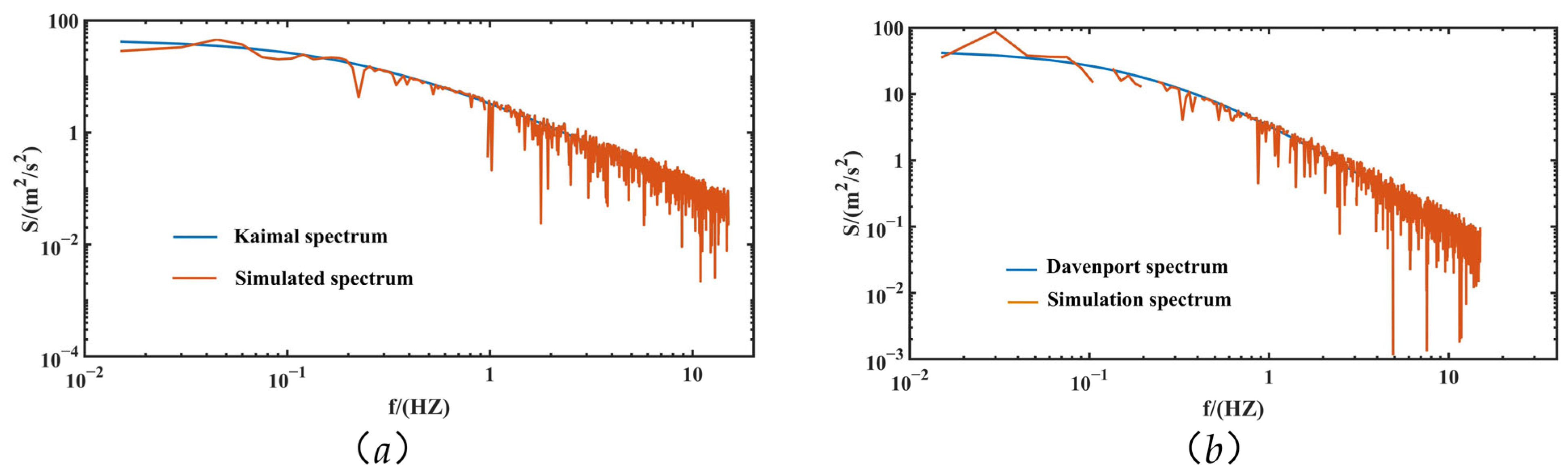
- An improved wind load model is proposed based on the weighted amplitude wave superposition (WAWS) method and the integral method in this paper.
- We have collected a real-world wind speed data set, which encompasses 31 continuously deployed wind sensors along the Qinghai-Tibet Railway in China (91°86′ E, 33°25′ N). The aforementioned data set encompasses almost all common running conditions of trains on the Qinghai-Tibet Railway under a strong wind environment. Based on this data set, we have verified the accuracy of our proposed pulsating wind model.
- Utilizing the conditional probability density function to design the dynamics evaluation criteria of trains.
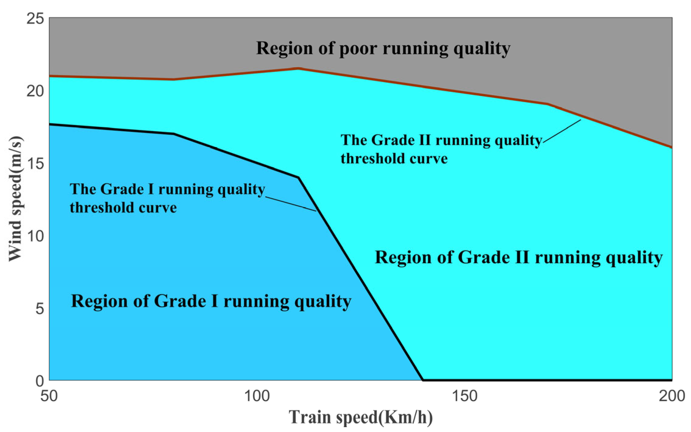
- The two-level running quality threshold curve of trains is constructed via the regularized regression model. On the premise of ensuring the safe operation of trains, the threshold curve of Grade-I can offer guidance for the smooth running of passenger trains. Likewise, the threshold curve of Grade-II can provide guidance for the efficient running of freight trains.
2. Methodology
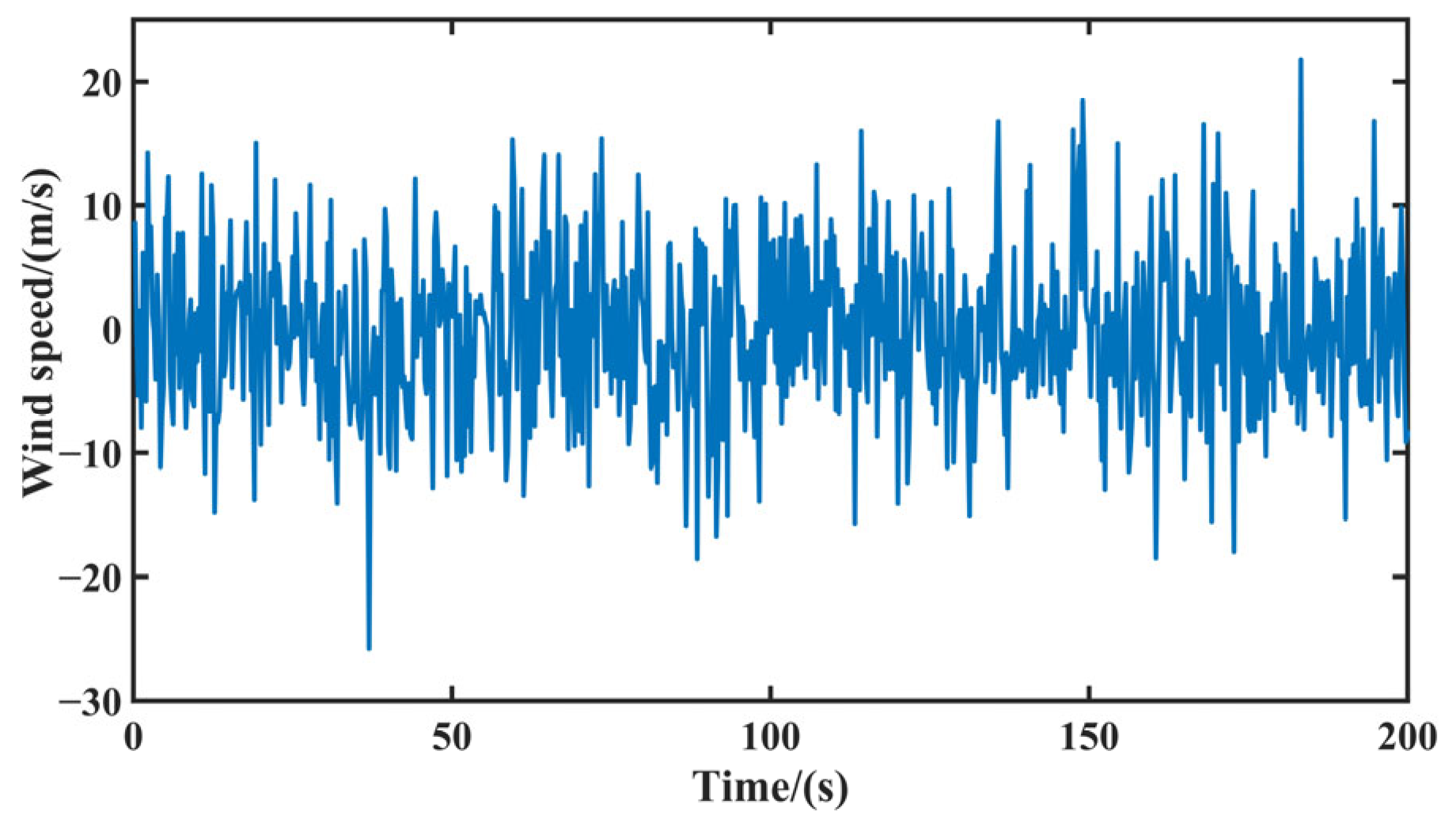
2.1. Simulation Method of Random Fluctuating Wind Field
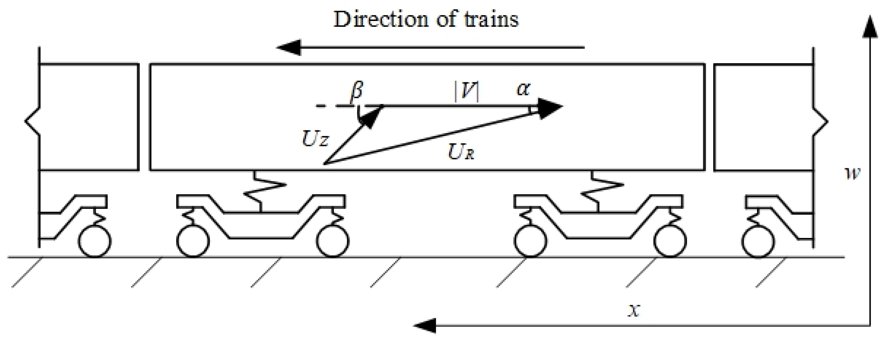
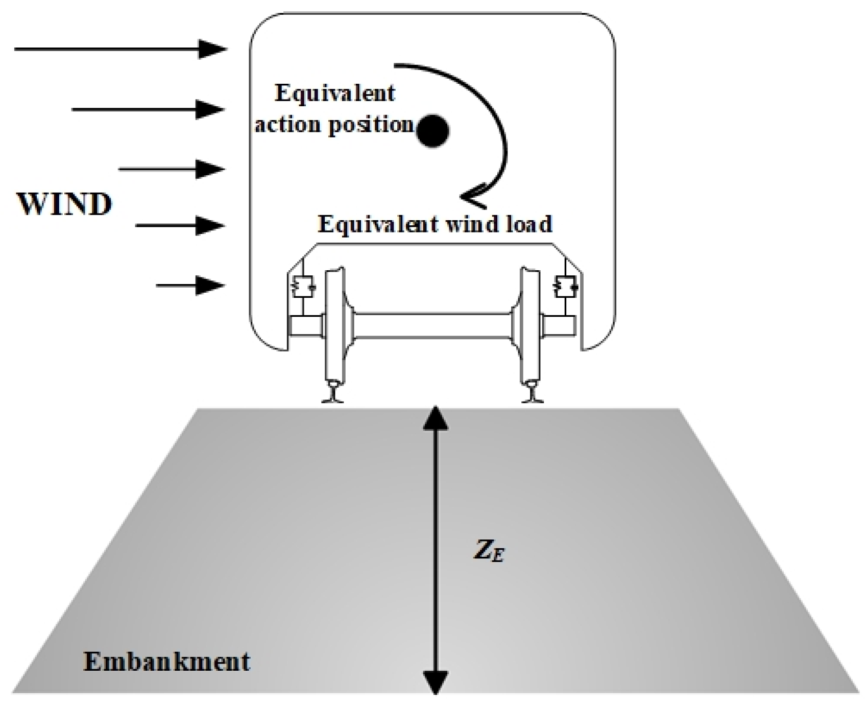
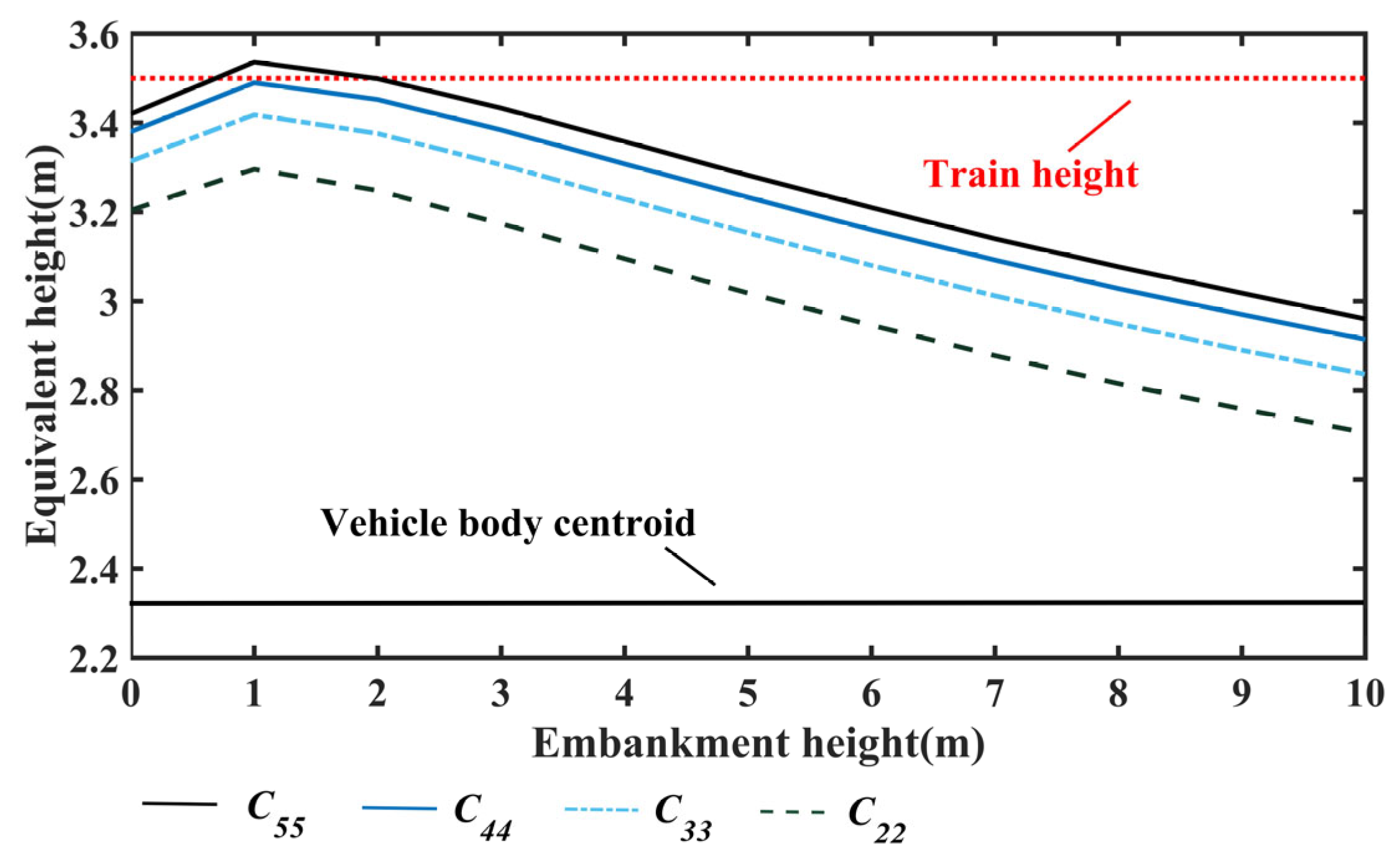
2.2. Calculation Method of Wind Load
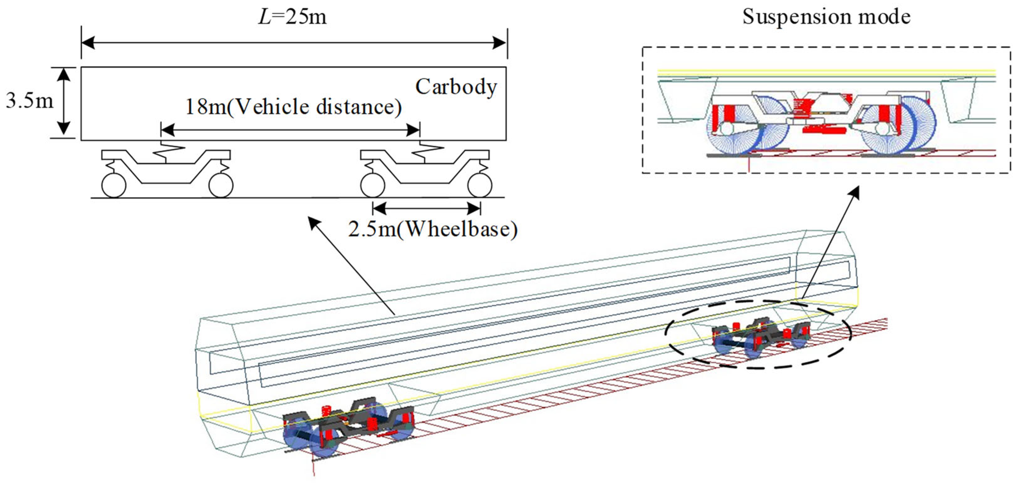
2.3. Multi-Body Dynamics Model
3. Simulation Experiments
3.1. Experiments
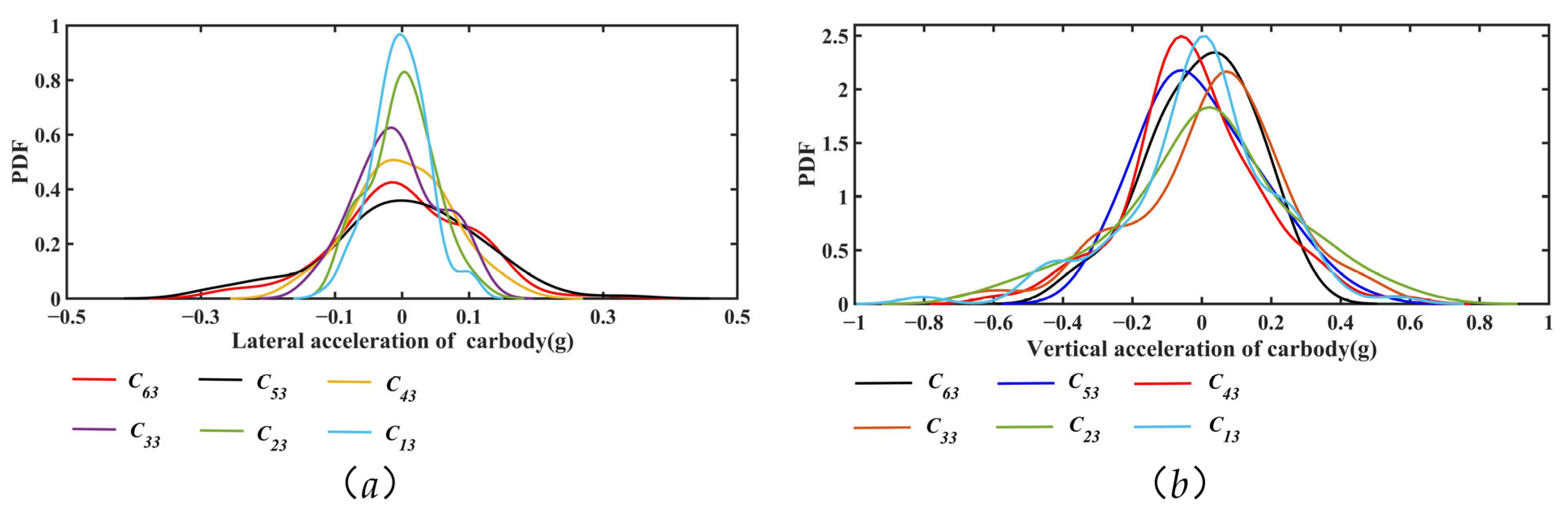
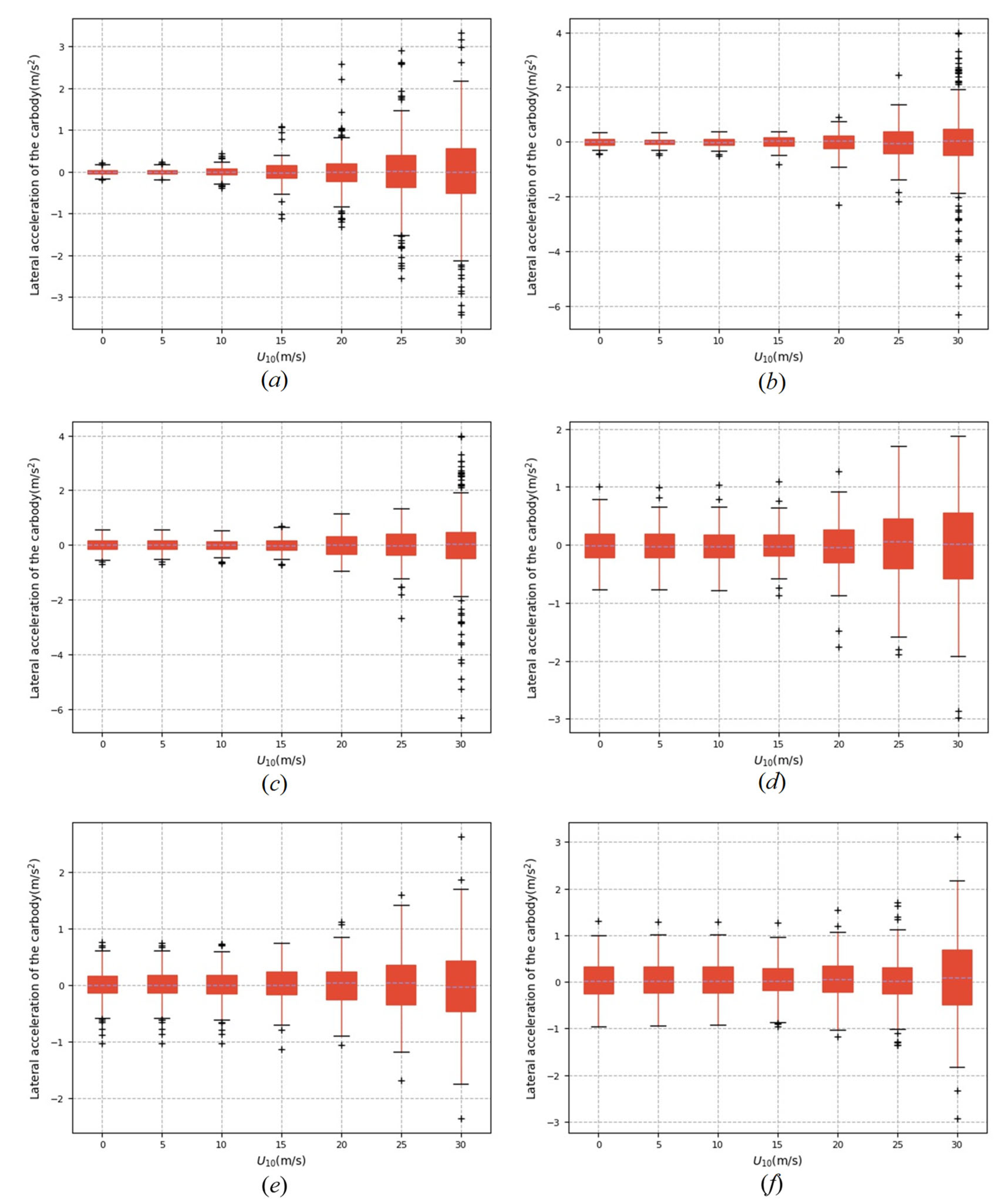
3.2. Results
4. Conclusions and Future Work
Author Contributions
Funding
Data Availability Statement
Conflicts of Interest
Abbreviations
| Symbol | Definition |
| The random time history of simulation point j | |
| Simulated pulsating wind time intervals | |
| The frequency increment | |
| Wind speed power spectrum | |
| Correlation coefficient matrix | |
| Fluctuating wind frequency | |
| Average wind speed at Z | |
| Angular frequency | |
| Random phase angle | |
| The number of simulated wind speed points | |
| The number of sample frequency points | |
| Cut-off frequency | |
| Turbulence standard deviation | |
| Turbulence integral scale | |
| Exponential attenuation coefficient | |
| Spacing of simulation points | |
| Wind load | |
| , where x is the longitudinal, u is the transverse, and w is the vertical | |
| Static wind load | |
| Buffeting load | |
| Air density | |
| Equivalent windward area | |
| Aerodynamic coefficient | |
| Shaking angle of wind direction | |
| Relative wind speed | |
| Train speed | |
| Train-to-wind angle | |
| Average wind speed at Zs | |
| Standard height | |
| Height of zero wind speed | |
| Mass matrix of the train model | |
| Damping matrix of the train model | |
| Stiffness matrix of the train model | |
| Displacement response | |
| Embankment height | |
| Distance between train body centroid and embankment | |
| Equivalent applied height of wind load | |
| Relative wind speed at h | |
| Equivalent average wind speed at train centroid | |
| Lateral acceleration function set for carbody | |
| Lateral acceleration of carbody under instance | |
| Maximum lateral acceleration | |
| Average lateral acceleration | |
| Max lateral acceleration | |
| Train’s Grade-I stability overrun probability | |
| Train’s Grade-II stability overrun probability | |
| Train exceedance probability function under different wind speeds | |
| Coefficient of function | |
| Validation set | |
| Regularization parameter | |
| Regularization function | |
| Cross-validation method |
References
- Chen, M.; Mao, J.; Xi, Y. Aerodynamic effect analysis of high-speed train entering and leaving single and double track tunnels under crosswind. Int. J. Rail Transp. 2023, 12, 304–326. [Google Scholar] [CrossRef]
- Bugalia, N.; Maemura, Y.; Ozawa, K. Organizational and institutional factors affecting high-speed rail safety in Japan. Saf. Sci. 2020, 128, 104762. [Google Scholar] [CrossRef]
- Song, Y.; Zhang, M.; Wang, H. A Response Spectrum Analysis of Wind Deflection in Railway Overhead Contact Lines Using Pseudo-Excitation Method. IEEE Trans. Veh. Technol. 2021, 70, 1169–1178. [Google Scholar] [CrossRef]
- Yu, M.; Pan, Z.; Liu, J.; Li, H. Operational Safety Assessment of a High-speed Train Exposed to the Strong Gust Wind. Fluid Dyn. Mater. Process. 2020, 16, 55–66. [Google Scholar] [CrossRef]
- Zhou, D.; Yu, D.; Wu, L.; Meng, S. Numerical investigation of the evolution of aerodynamic behaviour when a high-speed train accelerates under crosswind conditions. Alex. Eng. J. 2023, 72, 51–66. [Google Scholar] [CrossRef]
- Wang, L.; Zhang, X.; Han, Y.; Liu, H.; Hu, P.; Cai, C. A fast hybrid algorithm for the random vibration analysis of train-bridge systems under crosswinds. Eng. Struct. 2024, 299, 117107. [Google Scholar] [CrossRef]
- Sun, Z.; Lou, P.; Huang, X. Temperature gradient of ballastless track in large daily temperature difference region and its influence on dynamic responses of vehicle-track-bridge system. Alex. Eng. J. 2023, 85, 114–131. [Google Scholar] [CrossRef]
- Liu, D.; Wang, T.; Liang, X.; Meng, S.; Zhong, M.; Lu, Z. High-speed train overturning safety under varying wind speed conditions. J. Wind Eng. Ind. Aerodyn. 2020, 198, 104111. [Google Scholar] [CrossRef]
- Zhou, W.; Han, T.; Liang, X.; Bao, J.; Li, G.; Xiao, H.; Liu, D.; Liu, B. Load identification and fatigue evaluation via wind-induced attitude decoupling of railway catenary. Rev. Adv. Mater. Sci. 2021, 60, 377–403. [Google Scholar] [CrossRef]
- Yu, M.; Jiang, R.; Zhang, Q.; Zhang, J. Crosswind Stability Evaluation of High-Speed Train Using Different Wind Models. Chin. J. Mech. Eng. 2019, 32, 40. [Google Scholar] [CrossRef]
- Sprenger, M.; Schmidli, J.; Egloff, L. The Laseyer wind storm—Case studies and a climatology. Meteorol. Z. 2018, 27, 15–32. [Google Scholar] [CrossRef]
- Baker, C.J. The simulation of unsteady aerodynamic cross wind forces on trains. J. Wind Eng. Ind. Aerodyn. 2010, 98, 88–99. [Google Scholar] [CrossRef]
- Diedrichs, B. Studies of Two Aerodynamic Effects on High-Speed Trains: Crosswind Stability and Discomforting Car Body Vibrations Inside Tunnels. Ph.D. Thesis, KTH, School of Engineering Sciences (SCI), Aeronautical and Vehicle Engineering, Rail Vehicles, Stockholm, Sweden, 2006. [Google Scholar]
- Heleno, R.; Montenegro, P.A.; Carvalho, H.; Ribeiro, D.; Calcada, R.; Baker, C. Influence of the railway vehicle properties in the running safety against crosswinds. J. Wind Eng. Ind. Aerodyn. 2021, 217, 104732. [Google Scholar] [CrossRef]
- Brambilla, E.; Giappino, S.; Tomasini, G. Wind tunnel tests on railway vehicles in the presence of windbreaks: Influence of flow and geometric parameters on aerodynamic coefficients. J. Wind Eng. Ind. Aerodyn. 2022, 220, 104838. [Google Scholar] [CrossRef]
- Zhang, X.F.; Wang, X.K.; Pandey, M.D.; Sørensen, J.D. An effective approach for high-dimensional reliability analysis of train-bridge vibration systems via the fractional moment. Mech. Syst. Signal Process. 2021, 151, 107344. [Google Scholar] [CrossRef]
- Xu, L.; Zhang, Q.; Yu, Z.; Zhu, Z. Vehicle–track interaction with consideration of rail irregularities at three-dimensional space. J. Vib. Control 2020, 26, 1228–1240. [Google Scholar] [CrossRef]
- DI Gialleonardo, E.; Cazzulani, G.; Melzi, S.; Braghin, F. The effect of train composition on the running safety of low-flatcar wagons in braking and curving manoeuvres. Proc. Inst. Mech. Eng. Part F J. Rail Rapid Transit 2017, 231, 666–677. [Google Scholar] [CrossRef]
- Deng, C.; Zhou, J.; Thompson, D.; Gong, D.; Sun, W.; Sun, Y. Analysis of the consistency of the Sperling index for rail vehicles based on different algorithms. Veh. Syst. Dyn. 2019, 59, 313–330. [Google Scholar] [CrossRef]
- Giappino, S.; Rocchi, D.; Schito, P.; Tomasini, G. Cross wind and rollover risk on lightweight railway vehicles. J. Wind Eng. Ind. Aerodyn. 2016, 153, 106–112. [Google Scholar] [CrossRef]
- Dai, Y.; Dai, X.; Bai, Y.; He, X. Aerodynamic Performance of an Adaptive GFRP Wind Barrier Structure for Railway Bridges. Materials 2020, 13, 4214. [Google Scholar] [CrossRef]
- Liu, H.; Liu, C.; He, S.; Chen, J. Short-Term Strong Wind Risk Prediction for High-Speed Railway. IEEE Trans. Intell. Transp. Syst. 2021, 22, 4243–4255. [Google Scholar] [CrossRef]
- Liu, F.; Niu, J.-q.; Zhang, J.; Li, G.-X. Full-Scale Measurement of Micropressure Waves in High-Speed Railway Tunnels. J. Fluids Eng.-Trans. ASME 2019, 141, 034501. [Google Scholar] [CrossRef]
- Yu, M.; Liu, J.; Liu, D.; Chen, H.; Zhang, J. Investigation of aerodynamic effects on the high-speed train exposed to longitudinal and lateral wind velocities. J. Fluids Struct. 2016, 61, 347–361. [Google Scholar] [CrossRef]
- Xiang, H.; Li, Y.; Chen, S.; Hou, G. Wind loads of moving vehicle on bridge with solid wind barrier. Eng. Struct. 2018, 156, 188–196. [Google Scholar] [CrossRef]
- Gou, H.; Chen, X.; Bao, Y. A wind hazard warning system for safe and efficient operation of high-speed trains. Autom. Constr. 2021, 132, 103952. [Google Scholar] [CrossRef]
- Li, D.; Song, H.; Meng, G.; Meng, J.; Chen, X.; Xu, R.; Zhang, J. Dynamic characteristics of wheel-rail collision vibration for high-speed train under crosswind. Veh. Syst. Dyn. 2022, 61, 1997–2022. [Google Scholar] [CrossRef]
- Wang, T.; Kwok, K.C.S.; Yang, Q.; Tian, Y.; Li, B. Experimental study on proximity interference induced vibration of two staggered square prisms in turbulent boundary layer flow. J. Wind Eng. Ind. Aerodyn. 2022, 220, 104865. [Google Scholar] [CrossRef]
- Song, Y.; Zhang, M.J.; Oseth, O.; Rønnquist, A. Wind deflection analysis of railway catenary under crosswind based on nonlinear finite element model and wind tunnel test. Mech. Mach. Theory 2022, 168, 104608. [Google Scholar] [CrossRef]
- Jing, H.; Liao, H.; Ma, C.; Tao, Q.; Jiang, J. Field measurement study of wind characteristics at different measuring positions in a mountainous valley. Exp. Therm. Fluid Sci. 2020, 112, 109991. [Google Scholar] [CrossRef]
- Somoano, M.; Battistella, T.; Rodríguez-Luis, A.; Fernández-Ruano, S.; Guanche, R. Influence of turbulence models on the dynamic response of a semi-submersible floating offshore wind platform. Ocean Eng. 2021, 237, 109629. [Google Scholar] [CrossRef]
- Doubrawa, P.; Churchfield, M.J.; Godvik, M.; Sirnivas, S. Load response of a floating wind turbine to turbulent atmospheric flow. Appl. Energy 2019, 242, 1588–1599. [Google Scholar] [CrossRef]
- Rannik, Ü.; Vesala, T.; Peltola, O.; Novick, K.A.; Aurela, M.; Järvi, L.; Montagnani, L.; Mölder, M.; Peichl, M.; Pilegaard, K.; et al. Impact of coordinate rotation on eddy covariance fluxes at complex sites. Agric. For. Meteorol. 2020, 287, 107940. [Google Scholar] [CrossRef]
- IEC 61400-1; Wind Turbines Part 1: Design Requirements. IEC: Geneva, Switzerland, 2005.
- Tan, Q.L.; Xie, C. Comparison and Analysis of Permafrost Railway Subgrade Settlement Deformation Monitoring. In Proceedings of the International Conference on Vibration, Structural Engineering and Measurement (ICVSEM2012), Shanghai, China, 19–21 October 2012. [Google Scholar]
- Banerjee, A.; Chakraborty, T.; Matsagar, V. Dynamic analysis of an offshore monopile foundation used as heat exchanger for energy extraction. Renew. Energy 2019, 131, 518–548. [Google Scholar] [CrossRef]
- Meng, H.; Su, H.; Guo, J.; Qu, T.; Lei, L. Experimental investigation on the power and thrust characteristics of a wind turbine model subjected to surge and sway motions. Renew. Energy 2022, 181, 1325–1337. [Google Scholar] [CrossRef]
- Orellano, A.; Schober, M. On side-wind stability of high-speed trains. Veh. Syst. Dyn. 2003, 40, 143–159. [Google Scholar]
- Tian, H. Train Aerodynamics; China Railway Publishing House: Beijing, China, 2007. [Google Scholar]
- Wu, H.; Zhou, Z.-J. Study on aerodynamic characteristics and running safety of two high-speed trains passing each other under crosswinds based on computer simulation technologies. J. Vibroeng. 2017, 19, 6328–6345. [Google Scholar] [CrossRef]
- Xiao, X.; Li, J.; Wang, C.; Cai, D.; Lou, L.; Shi, Y.; Xiao, F. Numerical and experimental investigation of reduced temperature effect on asphalt concrete waterproofing layer in high-speed railway. Int. J. Rail Transp. 2022, 11, 389–405. [Google Scholar] [CrossRef]
- TB 10621-2009; Design Specification for High Speed Railway. TransForyou Co., Ltd.: Beijing, China, 2010.
- Alaeiyan, H.; Mosavi, M.R.; Ayatollahi, A. Improving the performance of GPS/INS integration during GPS outage with incremental regularized LSTM learning. Alex. Eng. J. 2024, 105, 137–155. [Google Scholar] [CrossRef]
- Zare, H.; Hajarian, M. Determination of regularization parameter via solving a multi-objective optimization problem. Appl. Numer. Math. 2020, 156, 542–554. [Google Scholar] [CrossRef]
- Budka, M.; Gabrys, B. Density-Preserving Sampling: Robust and Efficient Alternative to Cross-Validation for Error Estimation. IEEE Trans. Neural Netw. Learn. Syst. 2013, 24, 22–34. [Google Scholar] [CrossRef]
- Tian, G.; Gao, J.M.; Zhai, W.M. A method for estimation of track irregularity limits using track irregularity power spectrum density of high-speed railway. J. China Railw. Soc. 2015, 37, 83–90. [Google Scholar]


| Train Speed (Km/h) | Response | Average Speed of the Winds (m/s) | ||||||
|---|---|---|---|---|---|---|---|---|
| 0 | 5 | 10 | 15 | 20 | 25 | 30 | ||
| 50 | Amean | 0.0583 | 0.0623 | 0.1114 | 0.2118 | 0.2927 | 0.4902 | 0.7150 |
| Amax | 0.1904 | 0.1959 | 0.3900 | 1.0804 | 2.2092 | 2.6112 | 3.3500 | |
| Pε1 | 0 | 0 | 0 | 0 | 0.0960 | 0.2460 | 0.4500 | |
| Pε2 | 0 | 0 | 0 | 0 | 0.0300 | 0.1260 | 0.3000 | |
| 80 | Amean | 0.1135 | 0.1182 | 0.1325 | 0.1668 | 0.3048 | 0.5090 | 0.7514 |
| Amax | 0.4167 | 0.4160 | 0.4470 | 0.5028 | 0.9095 | 2.1728 | 4.4824 | |
| Pε1 | 0 | 0 | 0 | 0.0100 | 0.1100 | 0.2900 | 0.4200 | |
| Pε2 | 0 | 0 | 0 | 0 | 0.0300 | 0.0300 | 0.2800 | |
| 110 | Amean | 0.1745 | 0.1760 | 0.1876 | 0.2175 | 0.3601 | 0.5147 | 0.7490 |
| Amax | 0.6041 | 0.6131 | 0.6302 | 0.7140 | 0.9543 | 1.8032 | 5.2800 | |
| Pε1 | 0.0200 | 0.0200 | 0.0300 | 0.0600 | 0.1600 | 0.3300 | 0.4200 | |
| Pε2 | 0 | 0 | 0 | 0 | 0.0200 | 0.1600 | 0.2800 | |
| 140 | Amean | 0.2433 | 0.2463 | 0.2470 | 0.2584 | 0.3613 | 0.5316 | 0.7004 |
| Amax | 0.7863 | 0.8178 | 0.7831 | 0.8742 | 1.4853 | 1.8082 | 2.8564 | |
| Pε1 | 0.0500 | 0.0500 | 0.0500 | 0.0500 | 0.1900 | 0.3300 | 0.4700 | |
| Pε2 | 0.0100 | 0.0100 | 0.0100 | 0.0100 | 0.0400 | 0.2100 | 0.3100 | |
| 170 | Amean | 0.2510 | 0.2507 | 0.2620 | 0.2896 | 0.3255 | 0.4619 | 0.6239 |
| Amax | 0.8087 | 0.8035 | 0.9345 | 0.8677 | 1.0717 | 1.3770 | 2.3109 | |
| Pε1 | 0.0700 | 0.0600 | 0.0700 | 0.1200 | 0.1700 | 0.2700 | 0.4300 | |
| Pε2 | 0.0100 | 0.0100 | 0.0120 | 0.0100 | 0.0400 | 0.0900 | 0.2900 | |
| 200 | Amean | 0.3262 | 0.3268 | 0.3291 | 0.3305 | 0.3664 | 0.4573 | 0.7416 |
| Amax | 1.0067 | 1.0138 | 1.0147 | 0.9636 | 1.1910 | 1.6318 | 2.9297 | |
| Pε1 | 0.1700 | 0.1700 | 0.1700 | 0.1700 | 0.2100 | 0.2900 | 0.5200 | |
| Pε2 | 0.0300 | 0.0300 | 0.0300 | 0.0400 | 0.0800 | 0.1700 | 0.3100 | |
| Train Speed (Km/h) | Linear Regression Function | R-Square |
|---|---|---|
| 50 | 0.90 | |
| 80 | 0.90 | |
| 110 | 0.87 | |
| 140 | 0.86 | |
| 170 | 0.88 | |
| 200 | 0.90 |
| Train Speed (Km/h) | Linear Regression Function | R-Square |
|---|---|---|
| 50 | 0.92 | |
| 80 | 0.85 | |
| 110 | 0.92 | |
| 140 | 0.89 | |
| 170 | 0.86 | |
| 200 | 0.92 |
Disclaimer/Publisher’s Note: The statements, opinions and data contained in all publications are solely those of the individual author(s) and contributor(s) and not of MDPI and/or the editor(s). MDPI and/or the editor(s) disclaim responsibility for any injury to people or property resulting from any ideas, methods, instructions or products referred to in the content. |
© 2024 by the authors. Licensee MDPI, Basel, Switzerland. This article is an open access article distributed under the terms and conditions of the Creative Commons Attribution (CC BY) license (https://creativecommons.org/licenses/by/4.0/).
Share and Cite
Meng, G.; Meng, J. Dynamics Performance Research and Calculation of Speed Threshold Curve for High-Speed Trains Under Unsteady Wind Loads. Mathematics 2024, 12, 3780. https://doi.org/10.3390/math12233780
Meng G, Meng J. Dynamics Performance Research and Calculation of Speed Threshold Curve for High-Speed Trains Under Unsteady Wind Loads. Mathematics. 2024; 12(23):3780. https://doi.org/10.3390/math12233780
Chicago/Turabian StyleMeng, Gaoyang, and Jianjun Meng. 2024. "Dynamics Performance Research and Calculation of Speed Threshold Curve for High-Speed Trains Under Unsteady Wind Loads" Mathematics 12, no. 23: 3780. https://doi.org/10.3390/math12233780
APA StyleMeng, G., & Meng, J. (2024). Dynamics Performance Research and Calculation of Speed Threshold Curve for High-Speed Trains Under Unsteady Wind Loads. Mathematics, 12(23), 3780. https://doi.org/10.3390/math12233780