Abstract
In this study, we introduce an algorithm that utilizes the Haar wavelet collocation method to solve the time-dependent Emden–Fowler equation. This proposed method effectively addresses both linear and nonlinear partial differential equations. It is a numerical technique where the differential equation is discretized using Haar basis functions. A difference scheme is also applied to approximate the time derivative. By leveraging Haar functions and the difference scheme, we form a system of equations, which is then solved for Haar coefficients using MATLAB software. The effectiveness of this technique is demonstrated through various examples. Numerical simulations are performed, and the results are presented in graphical and tabular formats. We also provide a convergence analysis and an error analysis for this method. Furthermore, approximate solutions are compared with those obtained from other methods to highlight the accuracy, efficiency, and computational convenience of this technique.
Keywords:
Emden–Fowler type equations; numerical method; backward difference scheme; Haar wavelet method MSC:
35G30; 65M70; 65M06; 65T60
1. Introduction and Mathematical Preliminaries
Partial differential equations (PDEs) are essential mathematical instruments employed to describe a multitude of phenomena in engineering [1], physics [2,3], and other applied sciences [4]. Unlike ordinary differential equations, which focus on functions of a single variable, PDEs are inherently more complex and capable of modeling a broad spectrum of physical processes. They are vital for representing systems where changes occur with respect to multiple independent variables, such as time and space.
The study and application of PDEs are pivotal for technological advancement and the comprehension of natural phenomena (see [5]). By developing efficient methods to solve these equations, researchers can simulate and predict the behavior of intricate systems, leading to breakthroughs in fields such as aerospace engineering [6], climate modeling [7], biomedical engineering [8,9], and more.
Analytically solving PDEs is often challenging due to their complexity. Consequently, numerical methods like finite element analysis [10], finite difference methods [11], and spectral methods [12] are frequently utilized. Temimi et al. [13] used an iterative finite difference algorithm to solve a two-dimensional Bratu problem numerically. They employed the Newton–Raphson–Kantorovich approximation in function space and designed an iterative finite difference approach that provided a straightforward algorithm for computing the sequence of numerical solutions. Darvishi et al. [14] used a modification of the HPM technique to solve sine-Gordon and coupled sine-Gordon equations numerically. Darvishi [15] also used domain decomposition schemes to solve partial differential equations. These techniques approximate the solutions of PDEs through computational algorithms, enabling the resolution of real-world problems that are otherwise analytically intractable.
The time-dependent Emden–Fowler equations are a class of partial differential equations that arise in various scientific and engineering contexts, particularly in astrophysics, fluid dynamics, and thermal analysis. Named after the astronomers Robert Emden [16] and Richard Fowler [17], these equations are extensions of the classical Emden–Fowler equations, incorporating time as a dynamic variable to model evolving systems.
The classical Emden–Fowler equations typically describe static, spherically symmetric stellar structures [18,19] and other similar phenomena where spatial variables alone dictate the system’s behavior. When extended to include time dependency, these equations become powerful tools for analyzing the temporal evolution of systems under various physical conditions. This extension is crucial for understanding dynamic processes such as the thermal behavior of stars, gas dynamics in astrophysical contexts, and transient heat conduction in materials. In our work, we consider the Emden–Fowler heat-type equation [20] in the form
where is a nonlinear function or nonlinear heat source. This equation is solved subject to boundary conditions:
and initial condition
The time-dependent version of this equation incorporates the effect of time, allowing it to model evolving systems where properties like density, temperature, or pressure change dynamically over time. In (1), is the primary variable of interest, which could represent physical quantities like density, temperature, or gravitational potential. is a spatial coordinate often representing a radial distance in problems with spherical symmetry and is a time coordinate indicating that evolves over time or a related temporal parameter. Physically, is a measure of the concavity or curvature of in space and often appears in diffusion processes. represents a type of “damping” or scaling effect in radial diffusion processes. This could represent heat spreading from a central source, mass diffusing in a spherically symmetric object, or energy dissipating in a star. The term acts as a source or sink, adding or removing based on its current state and location. This term could represent reactions like chemical decay or fusion, heat generation in a stellar context.
A significant amount of research has been conducted to examine singular boundary value problems using various methods. Culham et al. [21] used the Galerkin method to solve time-dependent nonlinear boundary value problems. Netuzhylov et al. [22] used space–time meshfree collocation method (STMCM) to solve system of partial differential equations by a consistent discretization in both space and time. Dehgan [23] explored second-order finite difference methods for addressing a non-local boundary value problem in the two-dimensional diffusion equation with Neumann boundary conditions. Wazwaz et al. [24] used a modified Adomian decomposition method to solve time-dependent Emden–Fowler equations numerically with boundary conditions. Singh et al. [25] discussed the modified homotopy perturbation method for solving nonlinear and singular time-dependent Emden–Fowler type equations with the Neumann and Dirichlet boundary conditions. Mkhatshwa et al. [26] presented the bivariate spectral collocation method with the use of overlapping grids when applying the Chebyshev spectral collocation method. Bataineh et al. [27] solved time-dependent Emden–Fowler equations using the homotopy analysis method. Shahni [28] proposed the Berstein polynomial technique to numerically solve derivative-dependent Emden–Fowler equations with boundary conditions.
We are using a Haar wavelet collocation technique with backward difference scheme to solve Emden–Fowler heat-type equations with boundary conditions. The backward difference scheme [29] is a powerful numerical tool that offers stability, ease of implementation, and robustness, making it well suited for solving a variety of differential equations. The backward difference scheme can more easily handle complex boundary conditions compared to some explicit methods. This flexibility is important in accurately modeling physical systems with intricate boundary behaviors. Haar wavelet collocation method [30] offers a combination of simplicity, efficiency, adaptability, and accuracy, making it an attractive choice for solving differential equations in various scientific and engineering applications.
Combining the backward difference scheme’s stability with the spatial adaptivity of the Haar wavelet collocation method leads to a robust overall framework. This method tends to minimize numerical dispersion and oscillations that can occur in high-gradient regions. Thus, this method is robust for a wide range of PDE problems, particularly those with sharp features or requiring stability over long time simulations. It is well suited for problems with discontinuities or local features, as the Haar wavelet collocation can adapt to these with lower computational costs due to the sparsity of the resulting system.
Haar Wavelet
The Haar wavelet functions are simple and piecewise constant, making them easy to implement and compute. Haar wavelets are widely used in computer vision and image processing applications [31], including face detection [32] and pattern recognition. The Haar wavelet function is defined as:
where , , and . We define , and where J is the maximum resolution, s represents a dilation parameter, and Specifically, the Haar wavelet constitutes a square wave family that is orthogonal, generally written as
for and
For resolution, , the Haar function matrix is given by
We define the collocation points where we approximate any function as , for .
After putting values
The integrals of wavelets are defined as
where m is an integer.
Similarly, we can calculate
Haar wavelets have local support, which means they are non-zero only in a small region. This property reduces the computational complexity and increases efficiency, especially for problems with localized features. Haar wavelets are piecewise constant functions that can accurately represent functions with discontinuities, sharp gradients, or localized features, unlike Fourier or polynomial-based methods, which require many terms to capture these features accurately. The hierarchical structure of Haar wavelets allows for fast computations and efficient use of resources, which is beneficial for large-scale problems. The sparsity also simplifies the process of matrix inversion or solving linear systems, as fewer non-zero elements need to be processed, making it more computationally efficient compared to methods that result in dense matrices. The adaptive mesh refinement property of Haar wavelets is advantageous over finite difference or finite element methods, which may require uniform grids or more complex adaptivity schemes to capture localized phenomena accurately.
The structure of this study is organized as follows: Section 1 presents the introduction and outlines essential mathematical preliminaries. Section 2 details the procedure employed in this article. Section 3 explores the convergence and error analysis. Section 4 applies our procedure to various examples. Section 5 addresses the numerical simulation of these examples. Finally, Section 6 concludes with a summary of our findings.
2. Numerical Procedure
In this section, we present the implementation of our technique in solving Emden–Fowler heat-type equations with boundary conditions. First, we divide the interval into subintervals with length . Define for time , where
Again, integrating (9) from 0 to with respect to gives
Also, we use the backward difference scheme for the time-derivative term
After collocating points in (12), we have a system of algebraic equations. This system of equations was solved for Haar coefficients using Matlab software. The values of the Haar coefficients gave us the approximate solution.
3. Convergence and Error Analysis
In this section, we concentrate on the convergence analysis approximation of . Define , is a positive integer.
Theorem 1
([33]). Assume that the partial differential equation exists and is bounded in the interval . For , where and , then
where denotes approximate solution, denotes the exact solution, and
Proof.
The proof is given in [33]. □
Error Analysis
The maximum absolute error norm is defined as follows:
The and root-mean-square errors are defined as:
The Figure 1 shows the comparison of maximum absolute error, error, and error.
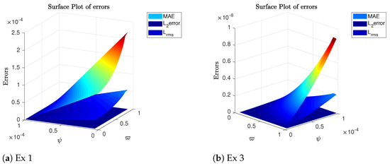
Figure 1.
Error plots of Example 1 and Example 3.
4. Applications
We know heat-type Emden–Fowler equations combine diffusion, damping, and nonlinear source or sink terms. We took examples with different source or sink terms and different damping factors.
4.1. Example 1
Consider the Emden–Fowler heat-type equation
with boundary conditions
The exact solution of (13) is
The factor in Example 1 adjusts the diffusion rate based on the radial position . The constant term is a uniform source term.
Then, we applied the Haar wavelet method and backward difference scheme to form a system of algebraic equations. That system was solved using MATLAB (latest v. 2024b) software to find the values of the Haar coefficients. Using the Haar coefficients, we found the numerical solution.
4.2. Example 2
Consider the Emden–Fowler heat-type equation
with boundary conditions
The exact solution of (14) is
The right side contains several terms, each representing source, sink, or external forcing terms that contribute independently to the dynamics of . Then, we applied the Haar wavelet method and backward difference scheme to form a system of algebraic equations. That system was solved using MATLAB software to find the values of the Haar coefficients. Using the Haar coefficients, we found the numerical solution.
4.3. Example 3
Consider the Emden–Fowler heat-type equation
with boundary conditions
The exact solution of (15) is
The exponential terms in the equation represent a nonlinear growth/decay, potentially modeling a reaction or feedback effect where an increase in accelerates its own growth. Then, we applied the Haar wavelet method and backward difference scheme to form a system of algebraic equations. That system was solved using MATLAB software to find the values of the Haar coefficients. Using the Haar coefficients, we found the numerical solution.
4.4. Example 4
Consider the Emden–Fowler heat-type equation
with boundary conditions
The exact solution of (16) is
Then, we applied the Haar wavelet method and backward difference scheme to form a system of algebraic equations. That system was solved using MATLAB software to find the values of the Haar coefficients. Using the Haar coefficients, we found the numerical solution.
5. Numerical Simulation
In this section, we present our numerical findings along with 2D and 3D graphs comparing the Haar solution and the exact solution. Figure 2 shows the error and comparison of exact and Haar solutions for Example 1. Figure 3 shows 3D surface plots of exact and Haar solutions for Example 1. Figure 4 shows 3D contour plots of exact and Haar solutions for Example 1. Figure 5 shows the error and comparison of exact and Haar solutions for Example 2. Figure 6 shows 3D surface plots of exact and Haar solutions for Example 2. Figure 7 shows 3D contour plots of exact and Haar solutions for Example 2. Figure 8 shows the error and comparison of exact and Haar solutions for Example 3. Figure 9 shows 3D surface plots of exact and Haar solutions for Example 3. Figure 10 shows 3D contour plots of exact and Haar solutions for Example 3. Figure 11 shows the error and comparison of exact and Haar solutions for Example 4. Figure 12 shows 3D surface plots of exact and Haar solutions for Example 4. Figure 13 shows 3D contour plots of exact and Haar solutions for Example 4. Table 1 gives us the numerical comparison of exact and Haar solutions for different for Example 1. Table 2 gives the error norm for different resolutions for Example1. Table 3 gives us the numerical comparison of exact and Haar solutions for different for Example 2. Table 4 gives us the numerical comparison of exact and Haar solutions for different for Example 3. In Table 5, we compare our results with other method for Example 3. Table 6 gives us the numerical comparison of exact and Haar solutions for different for Example 4. In Table 7, we compare our results with other methods and provide the CPU run time to demonstrate the efficiency and convenience of our approach.
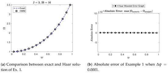
Figure 2.
Numerical simulation of Example 1.
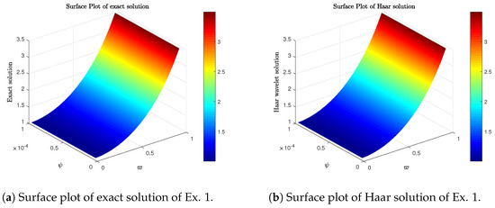
Figure 3.
Surface plots of Example 1.
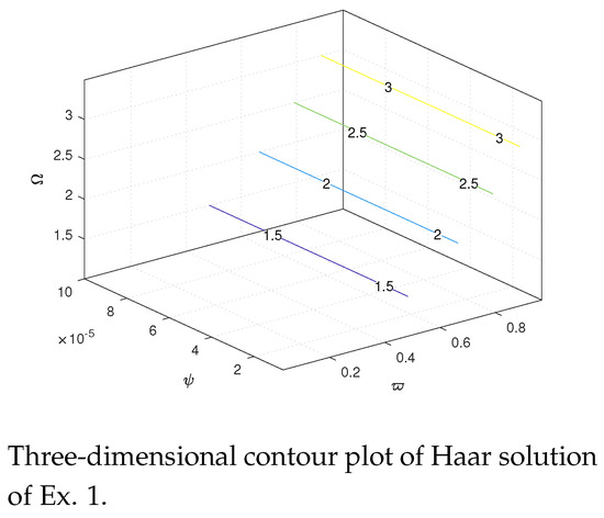
Figure 4.
Contour plot of Example 1.
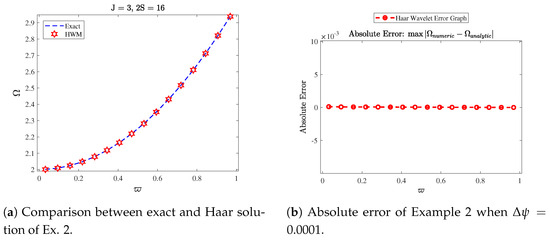
Figure 5.
Numerical simulation of Example 2.
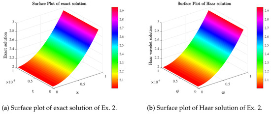
Figure 6.
Surface plots of Example 2.
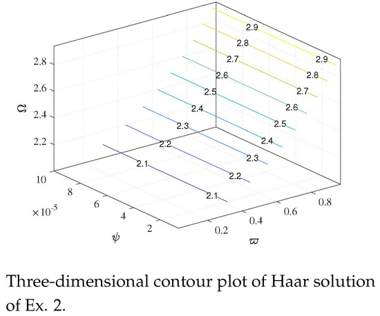
Figure 7.
Contour plot of Example 2.
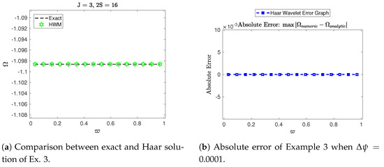
Figure 8.
Numerical simulation of Example 3.
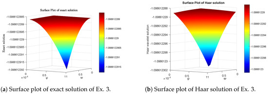
Figure 9.
Surface plots of Example 3.
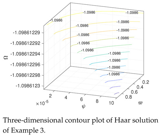
Figure 10.
Contour plot of Example 3.
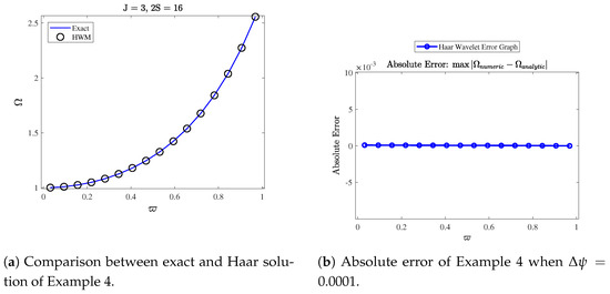
Figure 11.
Numerical simulation of Example 4.
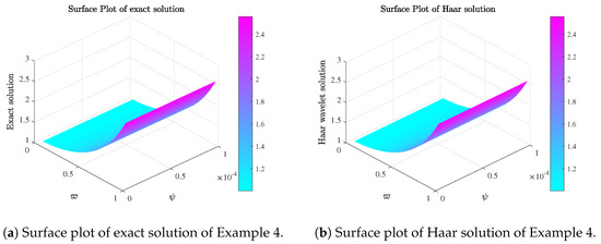
Figure 12.
Surface plots of Example 4.
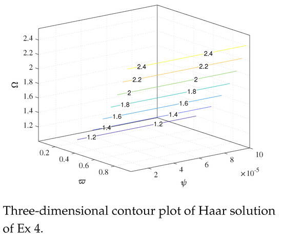
Figure 13.
Contour plot of Example 4.

Table 1.
Comparison of Haar solution and exact solution of Example 1 ( and ) when .
Table 2.
Error norm of Example 1 ().
Table 3.
Comparison of the Haar solution and exact solution of Example 2 ( and ) when .
Table 4.
Comparison of Haar solution and exact solution of Example 3 () when .
Table 5.
Comparison of Haar solution with MADM for Example 3.
Table 6.
Comparison of Haar solution and exact solution of Example 4 () when .
Table 7.
Comparison of Haar solution with other methods for Example 4.
6. Conclusions
The numerical solution of the time-dependent Emden–Fowler equation offers a powerful way to simulate and understand time-dependent processes. In diffusion processes, the numerical solution provides the density or concentration profile over time and space, showing how a substance diffuses or a population disperses under the influence of nonlinear effects. In plasma physics, solutions to the time-dependent Emden–Fowler equation are relevant to understanding plasma behavior in various configurations, such as spherical or cylindrical plasma distributions. The Haar wavelet collocation method, combined with a backward difference scheme, has proven to be an effective and efficient approach for solving time-dependent Emden–Fowler equations, including both linear and nonlinear partial differential equations. The flexibility of this method in handling complex boundary conditions makes it particularly suitable for modeling physical systems with intricate boundary behaviors. The numerical results, supported by 2D and 3D visual comparisons between the Haar solution and the exact solution, highlight the accuracy, adaptability, and computational efficiency of this technique.
Additionally, the use of Haar wavelets introduces several advantages, such as simplicity, local support, and sparse representation, which reduces computational complexity and improves efficiency. A comparative analysis, including CPU run time and error metrics, indicated that this method not only met but often surpassed the performance of alternative methods in terms of accuracy and computational convenience. In general, the Haar wavelet collocation method is a promising tool for solving differential equations in scientific and engineering applications due to its combination of precision, efficiency, and ease of implementation.
Author Contributions
P.G. spearheaded the investigation and coordinated the necessary literature. A.K. composed the manuscript, interpreted the findings, performed all numerical calculations, and generated the graphs. M.N.A., S.A. and A.F.A. compiled the data for tables, crafted the study site map, and formatted the final document. All authors have reviewed and consented to the published version of the manuscript.
Funding
The authors are thankful to the Deanship of Graduate Studies and Scientific Research at Najran University for funding this work under the Easy Funding Program grant code (NU/EFP/SERC/13/75-2).
Data Availability Statement
The original contributions presented in the study are included in the article, further inquiries can be directed to the corresponding author.
Acknowledgments
The authors are thankful to the Deanship of Graduate Studies and Scientific Research at Najran University for funding this work under the Easy Funding Program grant code (NU/EFP/SERC/13/75-2).
Conflicts of Interest
The authors declare no conflicts of interest.
Correction Statement
This article has been republished with a minor correction to the acknowledgments. This change does not affect the scientific content of the article.
References
- Ames, W.F. Nonlinear Partial Differential Equations in Engineering; Academic Press: Cambridge, MA, USA, 1965. [Google Scholar]
- Sommerfeld, A. Partial Differential Equations in Physics; Academic Press: Cambridge, MA, USA, 1949. [Google Scholar]
- Rubinstein, I.; Rubinstein, L. Partial Differential Equations in Classical Mathematical Physics; Cambridge University Press: Cambridge, UK, 1998. [Google Scholar]
- Zauderer, E. Partial Differential Equations of Applied Mathematics; John Wiley & Sons: Hoboken, NJ, USA, 2011. [Google Scholar]
- Salsa, S.; Vegni, F.; Zaretti, A.; Zunino, P. A Primer on PDEs: Models, Methods, Simulations; Springer Science & Business Media: Berlin/Heidelberg, Germany, 2013. [Google Scholar]
- Xia, H.; Tucker, P.; Dawes, W. Level sets for CFD in aerospace engineering. Prog. Aerosp. Sci. 2010, 46, 274–283. [Google Scholar] [CrossRef]
- Müller, E.H.; Scheichl, R. Massively parallel solvers for elliptic partial differential equations in numerical weather and climate prediction. Q. J. R. Meteorol. Soc. 2014, 140, 2608–2624. [Google Scholar] [CrossRef]
- Schiesser, W.E. Partial Differential Equation Analysis in Biomedical Engineering: Case Studies with MATLAB; Cambridge University Press: Cambridge, UK, 2013. [Google Scholar]
- Schiesser, W. Time Delay ODE/PDE Models: Applications in Biomedical Science and Engineering; CRC Press: Boca Raton, FL, USA, 2019. [Google Scholar]
- Johnson, C. Numerical Solution of Partial Differential Equations by the Finite Element Method; Courier Corporation: Chelmsford, MA, USA, 2009. [Google Scholar]
- Thomas, J.W. Numerical Partial Differential Equations: Finite Difference Methods; Springer Science & Business Media: Berlin/Heidelberg, Germany, 2013; Volume 22. [Google Scholar]
- Pedram, P.; Mirzaei, M.; Gousheh, S.S. Using spectral method as an approximation for solving hyperbolic PDEs. Comput. Phys. Commun. 2007, 176, 581–588. [Google Scholar] [CrossRef]
- Temimi, H.; Ben-Romdhane, M.; Baccouch, M.; Musa, M. A two-branched numerical solution of the two-dimensional Bratu’s problem. Appl. Numer. Math. 2020, 153, 202–216. [Google Scholar] [CrossRef]
- Darvishi, M.T.; Khani, F.; Hamedi-Nezhad, S.; Ryu, S.W. New modification of the HPM for numerical solutions of the sine-Gordon and coupled sine-Gordon equations. Int. J. Comput. Math. 2010, 87, 908–919. [Google Scholar] [CrossRef]
- Darvishi, M. Preconditioning and domain decomposition schemes to solve PDEs. Int. J. Pure Appl. Math. 2004, 15, 419–440. [Google Scholar]
- Emden, R. Gaskugeln: Anwendungen der Mechanischen Wärmetheorie auf Kosmologische und Meteorologische Probleme; BG Teubner: Leipzig, Germany, 1907. [Google Scholar]
- Fowler, R. Some results on the form near infinity of real continuous solutions of a certain type of second order differential equation. Proc. Lond. Math. Soc. 1914, 2, 341–371. [Google Scholar] [CrossRef]
- Chandrasekhar, S.; Chandrasekhar, S. An Introduction to the Study of Stellar Structure; Courier Corporation: Chelmsford, MA, USA, 1957; Volume 2. [Google Scholar]
- Kippenhahn, R.; Weigert, A.; Weiss, A. Stellar Structure and Evolution; Springer: Berlin/Heidelberg, Germany, 1990; Volume 192. [Google Scholar]
- Batiha, K. Approximate analytical solutions for time-dependent Emden-Fowler-type equations by variational iteration method. Am. J. Appl. Sci. 2007, 4, 439–443. [Google Scholar] [CrossRef]
- Culham, W.; Varga, R.S. Numerical methods for time-dependent, nonlinear boundary value problems. Soc. Pet. Eng. J. 1971, 11, 374–388. [Google Scholar] [CrossRef]
- Netuzhylov, H.; Zilian, A. Space–time meshfree collocation method: Methodology and application to initial-boundary value problems. Int. J. Numer. Methods Eng. 2009, 80, 355–380. [Google Scholar] [CrossRef]
- Dehghan, M. On the numerical solution of the diffusion equation with a nonlocal boundary condition. Math. Probl. Eng. 2003, 2003, 81–92. [Google Scholar] [CrossRef]
- Singh, R.; Wazwaz, A.M. Numerical solution of the time dependent Emden–Fowler equations with boundary conditions using modified decomposition method. Appl. Math. Inf. Sci. 2016, 10, 403–408. [Google Scholar] [CrossRef]
- Singh, R.; Singh, S.; Wazwaz, A.M. A modified homotopy perturbation method for singular time dependent Emden–Fowler equations with boundary conditions. J. Math. Chem. 2016, 54, 918–931. [Google Scholar] [CrossRef]
- Mkhatshwa, M.P.; Motsa, S.S.; Sibanda, P. Numerical solution of time-dependent Emden-Fowler equations using bivariate spectral collocation method on overlapping grids. Nonlinear Eng. 2020, 9, 299–318. [Google Scholar] [CrossRef]
- Bataineh, A.S.; Noorani, M.S.M.; Hashim, I. Homotopy analysis method for singular IVPs of Emden–Fowler type. Commun. Nonlinear Sci. Numer. Simul. 2009, 14, 1121–1131. [Google Scholar] [CrossRef]
- Shahni, J.; Singh, R. Numerical results of Emden–Fowler boundary value problems with derivative dependence using the Bernstein collocation method. Eng. Comput. 2022, 38, 371–380. [Google Scholar] [CrossRef]
- Bin Suleiman, M.; Binti Ibrahim, Z.B.; Bin Rasedee, A.F.N. Solution of Higher-Order ODEs Using Backward Difference Method. Math. Probl. Eng. 2011, 2011, 810324. [Google Scholar] [CrossRef]
- Šarler, B.; Aziz, I.; Fazal-i-Haq. Haar wavelet collocation method for the numerical solution of boundary layer fluid flow problems. Int. J. Therm. Sci. 2011, 50, 686–697. [Google Scholar]
- Mulcahy, C. Image compression using the Haar wavelet transform. Spelman Sci. Math. J. 1997, 1, 22–31. [Google Scholar]
- Satiyan, M.; Hariharan, M.; Nagarajan, R. Recognition of facial expression using Haar wavelet transform. J. Electr. Electron. Syst. Res. (JEESR) 2010, 3, 89–96. [Google Scholar]
- Zaman, S.S.; Amin, R.; Haider, N.; Akgül, A. Numerical solution of Fisher’s equation through the application of Haar wavelet collocation method. Numer. Heat Transf. Part B Fundam. 2024, 1–12. [Google Scholar] [CrossRef]
- Bataineh, A.S.; Isik, O.R.; Alomari, A.K.; Shatnawi, M.; Hashim, I. An efficient scheme for time-dependent Emden-Fowler type equations based on two-dimensional Bernstein polynomials. Mathematics 2020, 8, 1473. [Google Scholar] [CrossRef]
Disclaimer/Publisher’s Note: The statements, opinions and data contained in all publications are solely those of the individual author(s) and contributor(s) and not of MDPI and/or the editor(s). MDPI and/or the editor(s) disclaim responsibility for any injury to people or property resulting from any ideas, methods, instructions or products referred to in the content. |
© 2024 by the authors. Licensee MDPI, Basel, Switzerland. This article is an open access article distributed under the terms and conditions of the Creative Commons Attribution (CC BY) license (https://creativecommons.org/licenses/by/4.0/).