Aerospace Equipment Fault Diagnosis Method Based on Fuzzy Fault Tree Analysis and Interpretable Interval Belief Rule Base

Abstract

The stable operation of aerospace equipment is important for space safety, and the fault diagnosis of aerospace equipment is of practical significance. A fault diagnosis system needs to establish clear causal relationships and provide interpretable determination results. Fuzzy fault tree analysis (FFTA) is a flexible and powerful fault diagnosis method, which can deeply understand causes and fault mechanisms. The interval belief rule base (IBRB) can describe uncertainty. In this paper, an interpretable fault diagnosis model (FFDI) for aerospace equipment based on FFTA and the IBRB is presented for the first time. Firstly, the initial FFDI is constructed with the assistance of FFTA. Second, a model inference is implemented based on an evidential reasoning (ER) parsing algorithm. Then, a projection covariance matrix adaptive evolutionary strategy algorithm with an interpretability constraints (IP-CMA-ES) optimization algorithm is used for optimization. Finally, the effectiveness of the FFDI is verified by a flywheel dataset. This method ensures the completeness of the rule base and the interpretability of the model, avoids the problem of exploding certain combinations of rules, and is suitable for the fault diagnosis of aerospace equipment.

1. Introduction

Aerospace equipment usually operates in space environments with a multitude of uncertainties, characterized by a large scale and high complexity [1]. Its stable operation is crucial to space safety. However, the fault diagnosis of aerospace equipment faces unique challenges, including high real-time requirements and difficult data acquisition. For example, with high-speed rotating equipment such as flywheel systems, it plays an important role in the attitude control and energy storage of spacecraft. Material fatigue, vibration, and unbalance caused by high-speed rotation can affect spacecraft stability and mission success. The current research lacks unified fault diagnosis standards and efficient real-time data analysis methods, especially in the aspects of multi-fault concurrency and small fault detection. In addition, in the aerospace field, the acquisition of historical fault data is costly, limiting the accuracy and generalization ability of models. Therefore, it is necessary to find an effective fault diagnosis method for aerospace equipment and provide correct guidance for its operation.

At present, many scholars have studied the fault diagnosis of aerospace equipment, which can be divided into the black box model, white box model and gray box model. The black box model determines whether a device has a fault by observing its outputs under different input conditions, but the explanation ability is poor [2]. The white box model is a fault diagnosis method based on the internal structure and working principles of the equipment, which has high data requirements [3]. The gray box model, which comprehensively considers external observation data and internal information about the equipment, is a fault diagnosis method between the black box model and the white box model [4]. A grey box model is suitable for the fault diagnosis of aerospace equipment. This kind of model can not only use existing physical knowledge to build the basic framework of the system, but also calibrate and optimize the parameters by combining the data collected in the actual flight, so as to achieve an efficient and accurate fault location and interpretation under the condition that the system is not completely transparent. This semi-transparent method not only avoids the inexplicable problems that may be caused by the black box model, but also solves the limitations of the white box model, which requires high comprehensive system knowledge and has difficulty dealing with the complex and changeable actual flight environment, so as to ensure flight safety and system stability.

The belief rule base (BRB) is a typical gray box model. In 2006, Yang et al. [5] first proposed the concept of the BRB based on evidential reasoning (ER), which is widely used in the fields of risk assessment [6], fault diagnosis [7], etc. However, the BRB model is prone to combination rule explosion when there are too many complex attributes. To avoid this problem, He et al. [8] proposed interval belief rule base (IBRB). It is worth noting that the BRB itself is interpretable. However, in the process of model optimization, its own interpretability may be destroyed. In 2020, Cao et al. [9] systematically summarized the interpretable characteristics of BRBs, which can be used as guidelines for the establishment of BRBs. Therefore, an interpretable IBRB can be applied to the fault diagnosis modeling of aerospace equipment.

However, an IBRB usually relies on expert experience, which may make the rule base of an IBRB incomplete. This ultimately leads to obtaining an initial model that is not intuitive, and it may not be possible to judge the reasonableness of the model at this stage. In the fault diagnosis of aerospace equipment, experts often introduce fault tree analysis (FTA) or fuzzy fault tree analysis (FFTA) to obtain more comprehensive and accurate results [10,11,12,13]. FTA can identify events that lead to equipment faults. However, FTA has a limited ability to deal with ambiguous information. FFTA introduces fuzzy logic and fuzzy set theory on the basis of FTA. Therefore, FFTA is not only able to deal with the causal relationship between the faults but is also able to deal with the fuzziness of the information [14]. Therefore, one can consider using FFTA to help an IBRB to establish the causal relationship between faults. This will provide insight into the fault mechanism and determine more accurately the root cause that leads to equipment faults. It is worth noting that in order to be able to accurately diagnose faults and take appropriate measures, it is necessary to ensure a clear understanding of the decision-making process of BRB [15].

Based on this, an interpretability aerospace equipment fault diagnosis model (FFDI) based on an IBRB and FFTA is proposed in this paper. This model has the following three advantages. Firstly, FFTA has the ability to process fuzzy information, identifying factors that lead to faults and providing more comprehensive and accurate fault diagnosis results. Secondly, the BRB introduces an interval structure, which can effectively reduce the number of belief rules and avoid the problem of combinatorial rule explosion to some extent. Thirdly, a projection covariance matrix adaptive evolutionary strategy algorithm with an interpretability constraints (IP-CMA-ES) optimization algorithm is used to ensure the interpretability of the model. Although there may be some accuracy loss during the optimization process, this ensures the explanatory requirements of the model during the iteration process.

This article’s contributions are as follows: (1) The equivalence relationship between FFTA and the IBRB is constructed. By establishing a fuzzy fault tree to assist the expert knowledge modeling, it can not only ensure more a complete rule base but also accurately describe the fault mechanism. This helps determine the root cause of the fault. (2) An interpretable IBRB is constructed. The model not only makes advances in solving the combinatorial rule explosion problem; at the same time, interpretability is maintained throughout the construction, inference, and optimization process of the model. This means that the reasoning process and results of the model can be clearly explained. Finally, this model is successfully applied to the field of aerospace equipment fault diagnosis and will provide strong support for the operation and maintenance of aerospace equipment.

The paper is structured as follows. In Section 2, the BRB model is introduced. And two problems that need to be solved in the modeling process are described. In Section 3, this paper describes the inference and construction of the FFDI, the conversion mechanism of the IBRB and FFTA, and the interpretable optimization of the IP-CMA-ES optimization algorithm. In Section 4, a flywheel system dataset is used for an experimental demonstration, and the feasibility of the method proposed in this paper is proved by comparing the experimental results. In Section 5, summarizes the shortcomings of this paper and puts forward the goals for future development directions.

2. BRB and Problem

2.1. BRB Description

A BRB can resolve evidence conflict and describe global uncertainties, which can be described by the following equation.

$$\begin{array}{l}{R}^k:\\ If{u}_{1}is{X}_1\wedge u_{2}is{X}_2\wedge \dots \wedge u_{M}is{X}_M,u_1,u_2,\dots u_M,\\ Thenresultis\{(G_1,{\beta }_{1,k}),(G_2,{\beta }_{2,k}),\dots ,(G_N,{\beta }_{N,k})\},\\ withruleweight{\lambda }_k,\\ andattributeweight{\phi }_1,{\phi }_2,\dots ,{\phi }_M,\\ k\in \{1,2,\dots ,L\},{\displaystyle \sum _{j=1}^N{\beta }_{j,k}\le 1},\end{array}$$

(1)

where $R^k$ denotes the $k$-th belief rule, $u_1,u_2,\dots ,u_M$ denote the $i-th(i=1,2,\dots ,M)$ premise attribute as input, $M$ denotes the number of premise attributes, $X_1,X_2,\dots ,X_M$ denote the reference value corresponding to the premise attribute, $(G_1,{\beta }_{1,k}),(G_2,{\beta }_{2,k}),\dots ,(G_N,{\beta }_{N,k})$ are their corresponding belief distribution, ${\beta }_{1,k},{\beta }_{2,k},\dots ,{\beta }_{N,k}$ denote the belief degree of the $i$-th premise attribute in the $k$-th rule, ${\lambda }_k$ denotes the rule weight, and ${\phi }_1,{\phi }_2,\dots ,{\phi }_M$ denote the premise attribute weights, which are used to indicate the importance of the premise attribute.

The modeling steps of a BRB are as follows.

Step 1: Problem mechanism analysis. Identify the main factors affecting the problem, that is, the premise attributes.

Step 2: Set the reference point and reference value of the premise attribute, and set the reference value corresponding to the result. The reference point usually selects the location where most of the points are centrally distributed, including the upper and lower bounds of the values. The number of reference points is determined by the problem definition. The higher the number of reference points, the higher the accuracy, but the more complex the problem will be.

Step 3: Construct a belief table. A BRB builds the rule base by Cartesian product and the inference model by attribute weight, rule weight, and belief level.

The accuracy and interpretability of the BRB model is closely related to expert knowledge, so it is very important to improve the expert knowledge base to ensure the establishment of a complete rule base.

2.2. Problem Description

When constructing a fault model for aerospace equipment, it is necessary to ensure that the model is reasonable and effective throughout its life cycle. Therefore, the following two issues need to be addressed.

Problem 1.

How to achieve the equivalent conversion of FFTA and the IBRB.

Expert knowledge may not be sufficient to construct a complete rule base. In addition, the complex nature of aerospace equipment often leads to uncertain information. However, FFTA can not only visually demonstrate whether the modeling process is reasonable but also use the fuzzy set to help improve the comprehensiveness of the diagnostic result. Therefore, the FFTA mechanism can be used to construct a complete diagnostic model. It is important to note that in order to successfully implement IBRB modeling through FFTA, the equivalence between FFTA and IBRB must be established. In this paper, the mapping relationship between FFTA and IBRB is described using expression 2.

$$ConvertBRB(Input/Output,\vartheta )=Mapping(BaseEvent/TopEvent,\rho ),$$

(2)

where the functions $Mapping(\cdot )$ and $ConvertBRB(\cdot )$ represent the nonlinear mapping relationship between FFTA and IBRB. $Input$ denotes the premise attribute of the IBRB, $Output$ denotes the output result of the IBRB, and $\vartheta$ is the parameter set of the IBRB. $BaseEvent$ and $TopEvent$ are events in the FFTA and denote the parameter set of the FFTA.

Problem 2.

How to ensure the interpretability of the aerospace equipment fault diagnosis model throughout its life cycle.

Both the FFTA and IBRB proposed in this paper are interpretable. However, the interpretability of the model may be damaged during parameter optimization. Therefore, in order to ensure the interpretability of the model in the whole life cycle, it is necessary to design reasonable and effective interpretability constraints for the IBRB.

$$y=FFDI(u,\varpi ),$$

(3)

$$\{r|r_1,r_2,\dots ,r_f\},$$

(4)

$$\varpi =q(y,u,Q,U),$$

(5)

where $y$ is the aerospace equipment fault diagnosis result, $u$ is the input value in the model, $\varpi$ is the set of parameters in the modeling process, the interpretable constraints can be represented by the set $\{r|r_1,r_2,\dots ,r_f\}$, $f$ is the number of interpretable constraints, $Q$ is the set of parameters in the optimization process, and $U$ is the interpretable constraints.

3. Construction and Inference of FFDI

Aerospace equipment can encounter problems in its work at any time. For example, a flywheel system fault diagnosis faces multiple challenges such as location and coverage limitations and complex environmental factors. These problems not only increase the complexity and difficulty of diagnosis but also make the collected data highly ambiguous. Relying on these data for fault diagnosis may have a direct impact on the accuracy and reliability of the diagnosis results. The combination of FFTA and an interpretable IBRB can effectively address the multiple challenges in fault diagnosis. FFTA quantifies uncertainty in data through fuzzy logic to improve the accuracy of information. An interpretable IBRB integrates multiple sources of information through clear rules to ensure the transparency and reliability of the diagnostic results. This improves the data processing efficiency, reduces diagnostic delays, and ensures the stable operation of aerospace equipment.

The fuzzy fault tree is constructed starting from the basic event and then gradually analyzing the reason for the occurrence of the fault to finally obtain the top event [16]. The fuzzy fault tree can then be used to assist the expert knowledge base for the initial modeling. The conversion of FFTA and IBRB is a new approach. The overall structure of the FFDI proposed in this paper is shown in Figure 1.

3.1. IBRB Modeling for Aerospace Equipment Fault Diagnosis

The transformation between FFTA and IBRB is not direct; it requires a “bridge”, which can be provided by a Bayesian network (BN). This section describes the conversion process between FFTA and IBRB.

3.1.1. Analysis of the Conversion Mechanism Between FFTA and IBRB

FFTA is an analytical method that can be used in aerospace equipment fault diagnosis. It can analyze the fault propagation relationship between system components and the possible factors leading to the system fault [17]. The IBRB is a knowledge representation and inference method for uncertainty inference, which is designed to deal with the inference problems of uncertainty factors and combinatorial rule explosion. The FFTA and IBRB cannot be mapped directly, so it is necessary to construct an equivalent relationship between them by a BN, so that the FFTA and IBRB can be combined effectively.

• Conversion Analysis of FFTA and BN

Both FFTA and BNs are common methods of fault analysis. FFTA can describe the fault propagation path; its nodes represent events that may lead to a fault occurring. A BN is a directed acyclic graph model that describes the probabilistic correlation between variables. It describes the dependency relationship between variables by a simple probability distribution, whose nodes represent probability variables or events [18].

Both FFTA and BNs play an important role in fault analysis, and the correspondence between them can be visualized in

Table 1. Mapping relationship table between FFTA and Bayesian network.

FFTA	BN
Top/Base event	Child/Parent node
The input and output relationship between “and” and “or” gates	Arrow direction
Logic gate	Conditional probability distribution of nodes

and Figure 2.

2.

Conversion Analysis of IBRB and BN

An IBRB consists of an expert knowledge base, optimization algorithm, and ER inference machine. The ER constitutes a general link probabilistic inference process [19]. A BN is very useful in representing expert knowledge, identifying critical uncertainties, etc. [20]. The Bayesian rule established by Yang et al. [21] can be applied in the symmetric process in the ER paradigm, where each piece of evidence is described in the same belief distribution format. It can be seen that when events are independent of each other, the belief degree and conditional probability are equivalent; this can be described as follows:

$${\gamma }_{ab}={\displaystyle \frac{h_{ab}}{{\displaystyle \sum _{i=1}^N{h}_{ib}}}},a=1,\dots ,N,j=1,\dots ,l,$$

(6)

where $h_{ab}$ denotes the probability that the $b$-th detection result $e_b$ is expected to occur if the $a$-th hypothesis ${\xi }_a$ of evidence $e_0$ is true; that is, ${\gamma }_{ab}=\gamma (e_b|{\xi }_a,e_0),{\displaystyle \sum _{b=1}^L{h}_{ab}}=1$. ${\gamma }_{ab}$ denotes the belief degree that the detection result $e_b$ points to hypothesis ${\xi }_a$, and ${\displaystyle \sum _{b=1}^L{\eta }_{ab}}=1$.

Meanwhile, if all the detections used to generate the generalized likelihood $h_{\psi ,b}$ are independent, then Bayesian inference is equivalent to the ER inference.

$${\eta }_{\psi ,b}={\displaystyle \frac{h_{\psi ,b}}{{\displaystyle {\sum }_{j\subseteq \mathsf{\Theta }}{h}_{i,b}}}},\psi \subseteq \mathsf{\Theta },j=1,\dots ,l,$$

(7)

where $\psi$ represents a set of fault diagnosis propositions, $h_{\psi ,b}$ represents the generalized likelihood of the $b$-th detection result $e_b$ under proposition $\psi$, and ${\displaystyle \sum _{b=1}^l{h}_{\psi ,b}}=1,\psi \subseteq \mathsf{\Theta }=\{{\xi }_1,\dots ,{\xi }_N\}$. ${\gamma }_{\psi ,b}$ represents the belief degree that the detection result $e_b$ points to proposition $\psi$, and ${\displaystyle {\sum }_{\psi \subseteq \mathsf{\Theta }}{\gamma }_{\psi ,b}}=1,\psi \subseteq \mathsf{\Theta }=\{{\xi }_1,\dots ,{\xi }_N\}$.

It can be seen that the ER as the inference engine of the IBRB can help convert the IBRB to a BN. The corresponding relationship is visualized in

Table 2. Mapping relationship table between BN and IBRB.

BN	IBRB
Parent node/Child node	Input/Output
Conditional probability	Belief degree
Conditional probability distribution	Belief rule base

and Figure 3.

3.

Conversion Analysis of IBRB and FFTA

Based on the above analysis, it can be inferred that the FFTA and IBRB can establish an equivalence relationship by a BN. The mapping relationship between them is described below, and a more intuitive conversion diagram is given, as shown in Figure 4.

• In FFTA, the failure probability of the base event contains three fuzzy triangular numbers, which are divided into three groups corresponding to the parent node of the BN, which corresponds to the upper, intermediate, and lower bound in the IBRB input;
• In FFTA, the occurrence probability of the intermediate event contains three fuzzy triangular numbers, which are divided into three groups corresponding to the parent and child node of the BN, which are used as the input and output of the IBRB;
• In FFTA, the occurrence probability of the top event contains three fuzzy triangular numbers, which are divided into three groups corresponding to the child parent node of the BN, corresponding to the IBRB output.

In summary, it can be learned that FFTA is a way to help the IBRB acquire knowledge. This conversion space can be described by expression 8 as follows:

$$S(B,To,\epsilon )=S(input,outpit,\kappa ),$$

(8)

where $S(\cdot )$ is the conversion space between the FFTA and IBRB, $\epsilon$ is the parameter set in the process from FFTA to the conversion space, $To$ denotes the top event, $B$ denotes the base event, $input$ is the input of the IBRB, $output$ is the output of the IBRB, and $\kappa$ is the parameter set in the process from the conversion space to the IBRB.

3.1.2. The Conversion Rule of Different Gates from FFTA to IBRB

In FFTA, the logic gates include the “and” and “or” gates. In the “and” gate, the occurrence of any basic event causes the top event to occur. In “or” gates, the occurrence of all basic events will cause the top event to occur. Therefore, attention should be paid to distinguishing different logic gates when analyzing mapping relationships.

• Conditional Probability Representation of Different Logic Gates

The causality of the FFTA is described by a logic gate, and this process can be described by expression 9, where $p(\cdot )$ denotes the conditional probability, $LogicG(\cdot )$ denotes the logic gate, and $p(B_1),\dots ,p(B_n)$ denote the probability of the $i$-th base event.

$$p(T)=LogicG(p(B_1),\dots ,p(B_n)).$$

(9)

In the process of constructing the mapping relationship between FFTA and the BN, it is necessary to notice the difference in the calculation formulas of the transformation rules corresponding to the “and” gate and “or” gate. The conditional probability of nodes in the BN is transformed between the “and” gate and the “or” gate as follows.

In the process of constructing the mapping relationship between FFTA and the BN, it should be noted that the transformation rules corresponding to the “and” gate and the “or” gate are computed differently. The conditional probability of the node in the BN is transformed in the “and” and “or” gates as follows, respectively, where $u_i$ denotes the reference value of the $i$-th base event in the FFTA:

$$p(G|u_1,u_2,\dots ,u_n)={\displaystyle \prod _{i=1}^n{u}_i},$$

(10)

$$p(G|u_1,u_2,\dots ,u_n)={\displaystyle \sum _{i=1}^n{u}_i}.$$

(11)

2.

Description of the Conversion Rule for FFTA and IBRB

In the IBRB, the belief level of the input and output is obtained through a series of belief rules [22]. The process can be described by expression 12, where $BD(\cdot )$ denotes the function component of the belief level of the input and output, $BF(\cdot )$ denotes the belief rule composition function of the IBRB, and $bf(inpu{t}_1),\dots ,bf(inpu{t}_n)$ denote the belief levels of the $i$-th input and output.

$$BD(output)=BF(bf(inpu{t}_1),\dots ,bf(inpu{t}_n)).$$

(12)

In conclusion, the computational conversion process from FFTA to BN to IBRB can be obtained, and its expression is shown as follows:

$$LogicG(\cdot )=Conver{t}_F(BF(\cdot ),\rho ),$$

(13)

$$BF(\cdot )=Conver{t}_B(LogicG(\cdot ),\vartheta ),$$

(14)

where $Conver{t}_F$ denotes the conversion function of FFTA and $Conver{t}_B$ denotes the conversion function of the IBRB.

3.

The Activation Rule Mode of the IBRB

In the BRB, the rule-matching degree and the activation weight of the activated rule need to be calculated, the number of rules is derived by the Cartesian product [23]. Therefore, when there are too many complex attributes, the number of rules may explode, thus causing the combinatorial rule explosion problem. In the IBRB, the number of rules is obtained by summing the reference intervals of each reference point, which greatly reduces the number of rules [24]. For example, in

Table 3. Example of reference intervals for indicators.

Indicator 1	Indicator 2
[1,3]	[1,2]
[3,5]	[2,4]
[5,8]	[4,6]
[8,9]	[6,7]

, the reference value of indicator 1 and indicator 2 correspond to [1,3,5,8] and [1,2,4,6] respectively. In the BRB, this produces 4 * 4 = 16 rules, but the IBRB produces only 4 + 4 = 8 rules, which achieves an effective reduction of belief rules. To ensure the reliability of the model, it is necessary to ensure the activated rules are reliable, so activation rule reliability is used to evaluate it [25]. In this case, pay attention to how the activation rule reliability is calculated under different logic gates.

4.

The Relationship Between the Activation Rule Reliability of IBRB and the Logic Gate of FFTA.

Firstly, the belief rule expressions under different logic gates are described.

• Belief rule expressions under different logic gates;

Expressions 15 and 16 describe the belief rule for the IBRB in the “and” gate and the “or” gate, respectively.

$$\begin{array}{l}BeliefRule:\\ If{u}_1\in [m_1,n_1]\wedge u_2\in [m_2,n_2]\wedge \dots \wedge u_M\in [m_M,n_M],\\ Thenresultis\{(G_1,{\beta }_{1,k}),(G_2,{\beta }_{2,k}),\dots ,(G_N,{\beta }_{N,k})\},\\ withruleweight{\lambda }_k,\\ andrulereliablity{\zeta }_k,\\ andindicatorreliability{\delta }_1,{\delta }_2,\dots ,{\delta }_M,\\ ininterpretableconstraint{r}_1,r_2,\dots ,r_f,\\ k\in \{1,2,\dots ,L\},{\displaystyle \sum _{j=1}^N{\beta }_{j,k}\le 1},\end{array}$$

(15)

$$\begin{array}{l}BeliefRule:\\ If{u}_1\in [m_1,n_1]\vee u_2\in [m_2,n_2]\vee \dots \vee u_M\in [m_M,n_M],\\ Thenresultis\{(G_1,{\beta }_{1,k}),(G_2,{\beta }_{2,k}),\dots ,(G_N,{\beta }_{N,k})\},\\ withruleweight{\lambda }_k,\\ andrulereliablity{\zeta }_k,\\ andindicatorreliability{\delta }_1,{\delta }_2,\dots ,{\delta }_M,\\ ininterpretableconstraint{r}_1,r_2,\dots ,r_f,\\ k\in \{1,2,\dots ,L\},{\displaystyle \sum _{j=1}^N{\beta }_{j,k}\le 1},\end{array}$$

(16)

where $[m_1,n_1],[m_2,n_2],\dots ,[m_M,n_M]$ denote the reference interval of the reference point, ${\zeta }_k$ denotes the rule reliability, ${\delta }_1,{\delta }_2,\dots ,{\delta }_M$ denote indicator reliability, and $r_1,r_2,\dots ,r_f$ denote the interpretable constraints. In the logic gates, “and” is denoted by $\wedge$, and “or” is denoted by $\vee$.

• Calculation of the activation rule reliability corresponding to different logic gates.

When calculating the activation rule reliability, it is crucial to consider whether events activate the rule through the “and” gate or the “or” gate. Expressions 17 and 18 calculate the activation rule reliability in the case of “and” gate and “or” gate transitions, respectively.

$$\alpha =[1-{\displaystyle \prod _{i=1}^M(1-{\delta }_i)}]*\chi ,$$

(17)

$$\alpha ={\displaystyle \sum _{i=1}^M{\delta }_i}-{\displaystyle \sum _{i=1}^M[{\delta }_i}*{\displaystyle \sum _{j=i+1}^M{\delta }_j})+{\displaystyle \sum _{i=1}^M({\delta }_i}*{\delta }_{i+1}*{\displaystyle \sum _{j=i+2}^M{\delta }_j})]*\chi ,$$

(18)

$$\chi =\left|{\beta }_1^2-{\beta }_2^2-\dots -{\beta }_N^2\right|,$$

(19)

where $\alpha$ represents the activation rule reliability and $\chi$ represents the belief factor, which is the absolute value of the difference between the squares of the belief values.

3.1.3. IBRB for Fault Diagnosis of Aerospace Equipment Is Constructed

The faults in the aerospace equipment are often caused by interactions between multiple components and variables. The ER, as the inference engine for the IBRB, can capture fuzziness, incompleteness, and a nonlinear causality. This can be applied to complex nonlinear input–output relationships in aerospace equipment [26].

In this section, the flywheel dataset in the experimental part is taken as an example. The fuzzy fault tree is built step by step to analyze the fault cause. When the initial data can be relied upon, the occurrence probability of the top event can be calculated from the failure probability of the base event. The complete fuzzy fault tree is shown in Figure 5.

3.2. IBRB Reasoning Process for Aerospace Equipment Fault Diagnosis

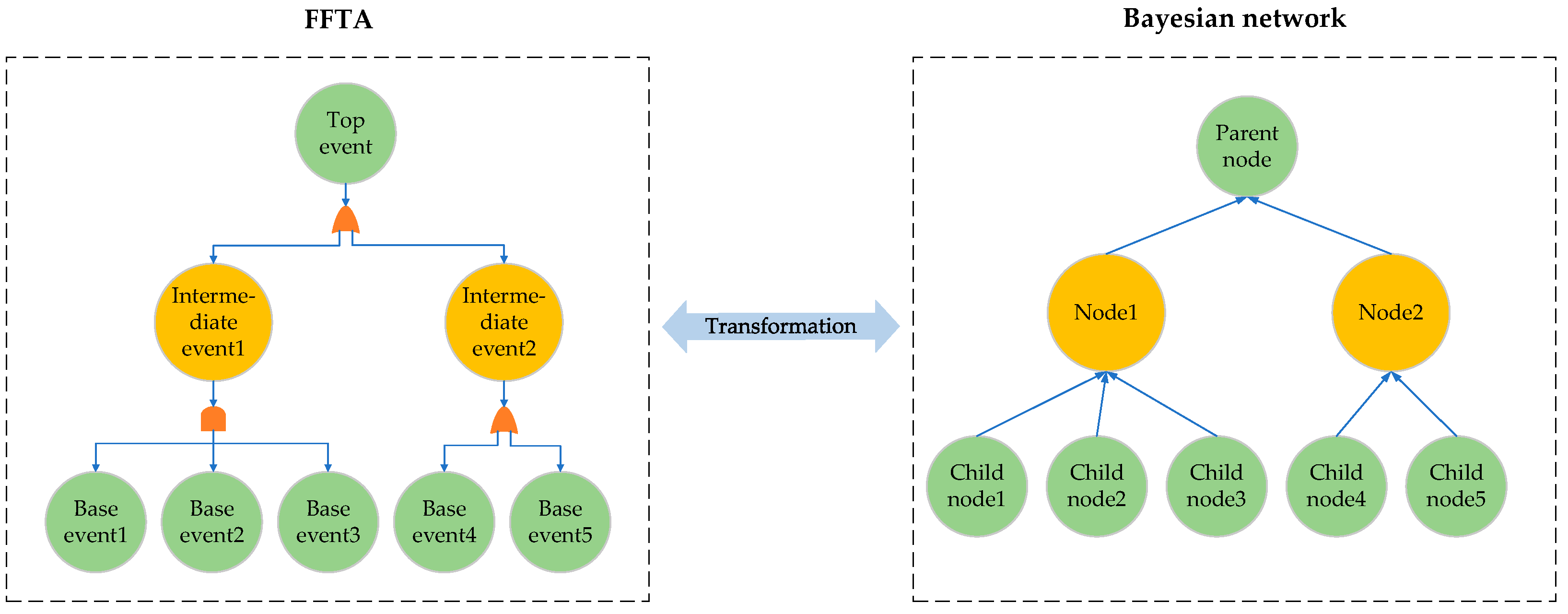
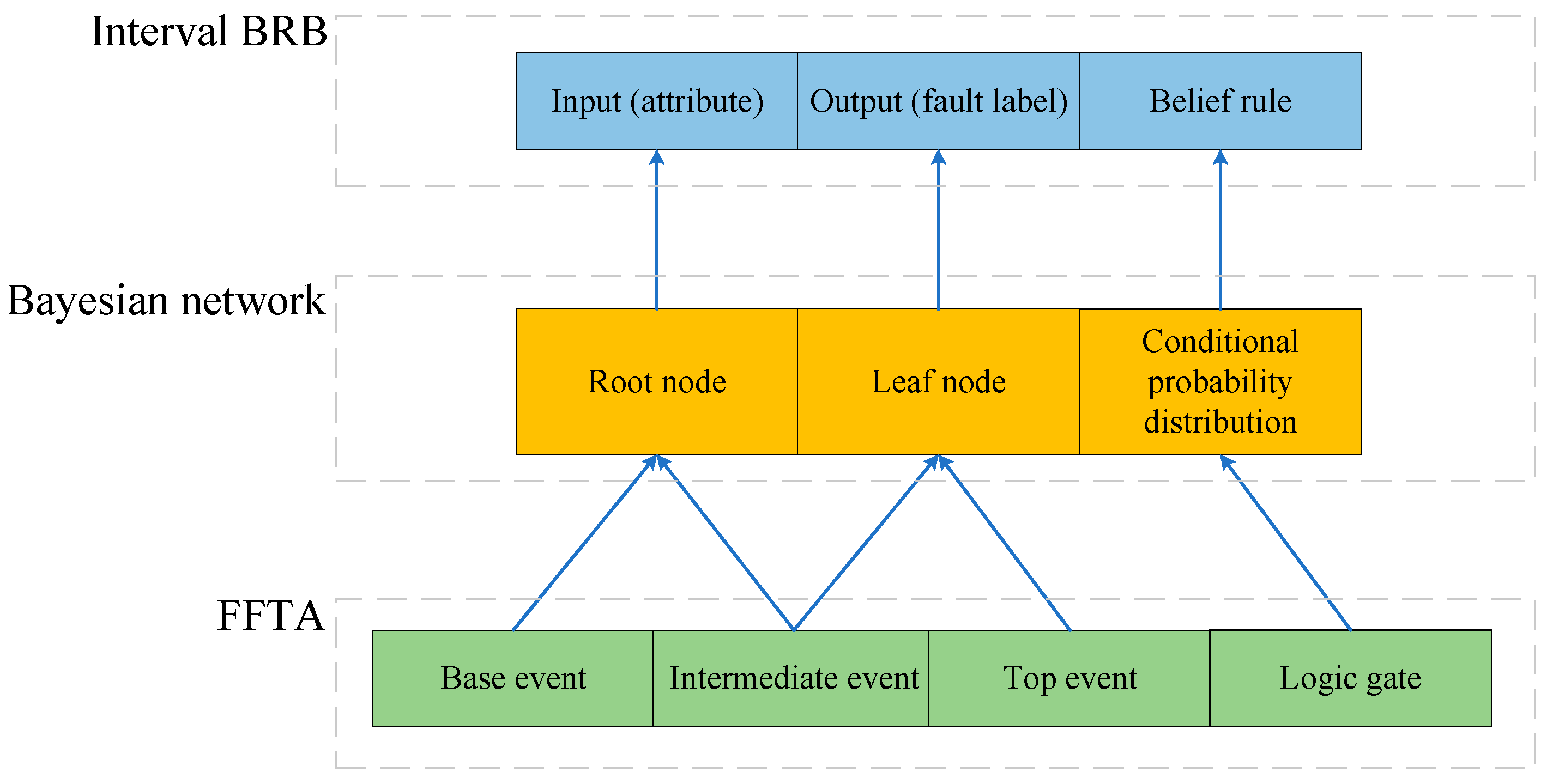
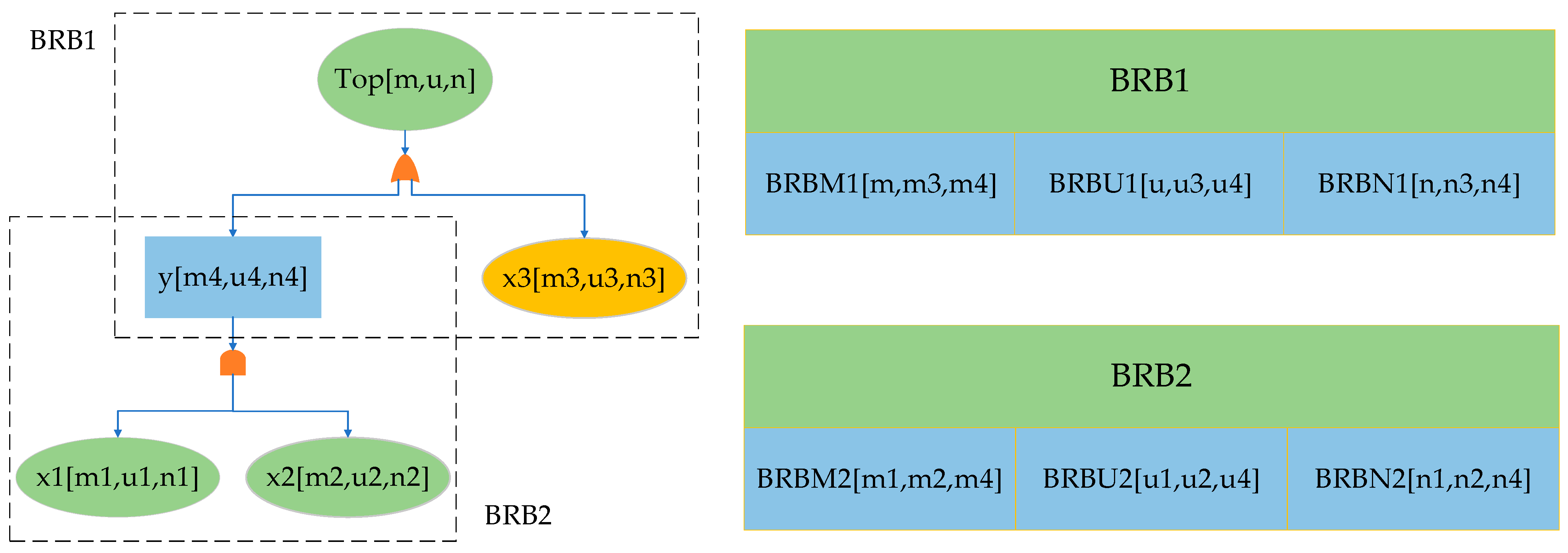
The FFDI represents the probability of an event through the fuzzy triangular number of FFTA. The fuzzy triangle number is divided into three groups, representing the upper limit, the lower limit, and the reference value, respectively. This can correspond to the reference intervals in the IBRB. After the data in FFTA are transformed to IBRB by the BN, the model is optimized for the fitting effect of the triangular fuzzy number of the top event probability. The conversion mechanism between FFTA, BN, and IBRB is used to solve the problem that expert knowledge is difficult to embed [27]. Figure 6 shows a schematic diagram of the model reasoning process.

After normalizing the data, the belief distribution is described as follows:

$$\begin{array}{l}{e}_i=\{(G_n,{\beta }_{n,i}),n=1,\dots ,N;(\mathsf{\Theta },{\beta }_{\mathsf{\Theta },i})\},\\ 0\le {\beta }_{n,i}\le 1,{\displaystyle \sum _{n=1}^N{\beta }_{n,i}\le 1},\end{array}$$

(20)

where ${\beta }_{n,i}$ denotes the belief degree that the fault diagnosis solution is assessed as $G_n$ under evidence $e_i$, ${\beta }_{\mathsf{\Theta },i}$ denotes global ignorance, and $\mathsf{\Theta }$ denotes the identification framework, which consists of $N$ assessment levels $\{G_1,G_2,\dots ,G_N\}$.

The evidence weight is denoted by $e{w}_i\in [0,1]$, and the evidence reliability is denoted by $e{d}_i\in [0,1]$. The new belief distribution is generated by mixing and weighting $e{w}_i$ and $e{d}_i$ as follows:

$$m_i=\{(G_n,{\stackrel{\sim }{m}}_{n,i}),\forall G_n\subseteq \mathsf{\Theta };({\beta }_{\mathsf{\Theta }},{\stackrel{\sim }{m}}_{{\beta }_{\mathsf{\Theta }},i})\},$$

(21)

$${\stackrel{\sim }{m}}_{n,i}=\left\{\begin{array}{ll}\hfill 0,\hfill & G_n=\varnothing \\ \hfill f_{dw,i}{m}_{n,i},\hfill & G_n\subseteq \mathsf{\Theta },G_n\ne \varnothing \\ \hfill f_{dw,i}(1-e{d}_i),\hfill & G_n=\beta (\mathsf{\Theta })\end{array}\right.$$

(22)

$$f_{dw,i}=1/(1+e{w}_1-e{d}_i),$$

(23)

$$m_{n,i}=e{w}_i{\beta }_{n,i},$$

(24)

where $m_{n,i}$ denotes the basic probability mass, ${\stackrel{\sim }{m}}_{n,i}$ represents the mixed probability mass of the $i$-th evidence under the evaluation level $G_n$, and $f_{dw,i}$ denotes the normalization factor, which satisfies ${\displaystyle \sum _{n=1}^N{\tilde{m}}_{n,i}+}{\tilde{m}}_{\beta (\mathsf{\Theta }),i}=1$.

The joint support ${\beta }_{n,e(L)}$ of $L$ independent evidence is calculated as below.

$$\forall G_n\in \mathsf{\Theta },\stackrel{\wedge }{m_{n,e(k)}=[(1-{\lambda }_k)m_{n,e(k-1)}+m_{\beta (\mathsf{\Theta }),e(k-1)}{m}_{m,k}]+{\displaystyle \sum _{A\cap B=G_n}{m}_{A,e(k-1)}{m}_{B,k}}},$$

(25)

$${\stackrel{\wedge }{m}}_{\beta (\mathsf{\Theta }),e(k)}=(1-{\zeta }_k)m_{\beta (\mathsf{\Theta }),e(k-1)},$$

(26)

$$m_{n,e(k)}=\left\{\begin{array}{ll}\hfill 0,\hfill & G_n=\varnothing \\ \hfill {\displaystyle \frac{{\stackrel{\wedge }{m}}_{n,e(k)}}{{\displaystyle \sum _{A\subseteq \mathsf{\Theta }}{\stackrel{\wedge }{m}}_{A,e(k)}+{\stackrel{\wedge }{m}}_{\beta (\mathsf{\Theta }),e(k)}}}},\hfill & G_n\ne \varnothing \end{array}\right.$$

(27)

$${\beta }_{n,e(k)}=\left\{\begin{array}{ll}\hfill 0,\hfill & G_n=\varnothing \\ \hfill {\displaystyle \frac{{\stackrel{\wedge }{m}}_{n,e(k)}}{{\displaystyle \sum _{A\subseteq \mathsf{\Theta }}{\stackrel{\wedge }{m}}_{A,e(k)}}}},G_n\subseteq \mathsf{\Theta },\hfill & G_n\ne \varnothing \end{array}\right.$$

(28)

where after fusing the first $n$ pieces of evidence, the belief degree for assessment level $G_n$ is denoted by ${\beta }_{n,e(k)}(k=1,2,\dots ,L)$, and the formula satisfies $m_{n,e(1)}=m_{n,1},m_{\beta (\mathsf{\Theta }),e(1)}=m_{\beta (\mathsf{\Theta }),1}$.

In summary of the above analysis, the following output belief distribution and expected utility value can be obtained:

$$e(L)=\{(G_n,{\beta }_{n,e(L)}),n=1,\dots ,N,(\mathsf{\Theta },{\beta }_{\mathsf{\Theta },e(L)}\},$$

(29)

$$y={\displaystyle \sum _{n=1}^{N}v(G_n){\beta }_{n,e(L)}+v(\mathsf{\Theta })}{\beta }_{\mathsf{\Theta },e(L)},$$

(30)

where $y$ represents the expected utility value, that is, the predicted output. $v(G_n)$ represents the utility value at evaluation level $G_n$.

In conclusion, the IBRB inference process for aerospace equipment fault diagnosis can be obtained as follows.

Step 1: Define the reference interval value.

Step 2: After inputting the initial parameter, determine the interval in which the parameter falls, and activate its corresponding rule according to this interval.

Step 3: Calculate the activation rule reliability corresponding to the current logic gate. The calculation formula in “and” gates is shown in expression (17) and that in “or” gates is shown in expression (18).

Step 4: The belief level of the fault diagnosis result is calculated.

Step 5: Calculate the expected utility value of the output.

3.3. Optimization of the FFDI Using the IP-CMA-ES Algorithm

In the experimental process, the initial parameters are established by experts based on historical experience [28]. The accuracy of the initial model cannot be guaranteed. Therefore, the model parameters must be optimized by the optimization algorithm. Among the current optimization algorithms, the projection covariance matrix adaptive evolution strategy algorithm (P-CMA-ES) has characteristics such as a high convergence speed, high precision, and diffusion rotational invariance. It is widely used in various BRB models [29]. Therefore, the FFDI can be optimized by the P-CMA-ES algorithm.

However, when the P-CMA-ES algorithm is used to optimize parameters, more emphasis is placed on the model accuracy, which may destroy the interpretability of the IBRB itself [30]. It may produce errors that contradict common sense during optimizing. For example, suppose that are three evaluation levels for aerospace equipment fault diagnosis, “unqualified”, “medium”, and “excellent”, if the model output is {(unqualified, 0.4), (medium, 0.2), (excellent, 0.4)}. It is obvious that the belief degree at both ends is higher than the belief degree in the middle. It violates the practical significance of the model and should not exist. In summary, the belief distribution should not be “concave”. As shown in Figure 7, when the optimized belief distribution is increasing, decreasing, or “convex”, the belief distribution can be considered reasonable; when the belief distribution is “concave”, the belief distribution is not reliable. In this case, the model parameter needs to be reoptimized until the actual belief distribution is generated [31].

To solve this problem, the P-CMA-ES algorithm is improved. That is, constraint conditions are introduced. First, the upper and lower threshold can be set to ensure that the belief degree is between them to make the assessment level effective, which can rule out unqualified data [32]. Then the belief degree can be normalized to guarantee that it sums to one. This can generate a reasonable belief distribution.

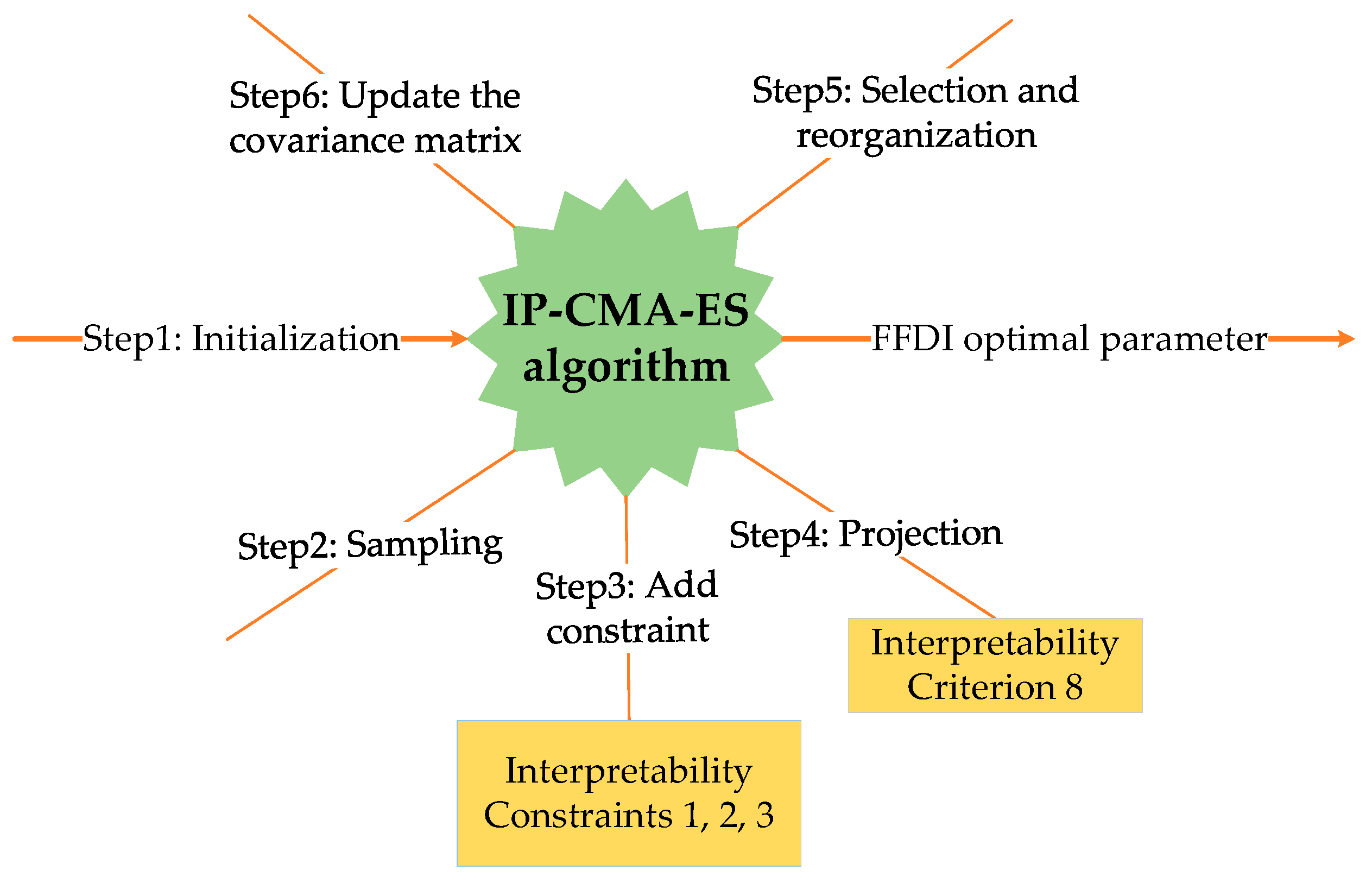
This section describes the optimization mechanism and the procedure of the IP-CMA-ES algorithm. The FFDI optimization structure is shown in Figure 8.

First, it needs to construct an objective function for the optimization model, which can be represented as follows:

$$\begin{array}{l}minMSE(\beta ,\zeta ,\lambda ),\\ \mathrm{s}.\mathrm{t}.{\displaystyle \sum _{n=1}^N{\beta }_{n,k}=1,}\\ 0\le {\beta }_{n,k}\le 1,n=1,\dots ,N,\\ 0\le {\zeta }_i\le 1,i=1,\dots ,L\\ 0\le {\lambda }_k\le 1,k=1,\dots ,L\end{array}$$

(31)

$$MSE(\beta ,\zeta ,\lambda )={\displaystyle \frac{1}{O_T}}{\displaystyle \sum _{k=1}^T{(y-y^{\#})}^2},$$

(32)

where $MSE(\cdot )$ is the deviation degree between the utility value output of the FFDI and the actual value, $O_T$ represents the number of training samples, and $y^{\#}$ represents the actual output result of the model.

The steps of the IP-CMA-ES algorithm are described in detail as follows:

Step 1: Initialization. The parameter set to be optimized is described, which includes the belief degree, rule reliability, and rule weight.

$${\omega }^0={\mathsf{\Omega }}^0\{{\beta }_{1,1},\dots ,{\beta }_{1,1},{\zeta }_1,\dots ,{\zeta }_L,{\lambda }_1,\dots ,{\lambda }_L\}.$$

(33)

Step 2: Sampling. The parameter for each generation can be obtained by sampling, and the formula is described below.

$${\mathsf{\Omega }}_i^{d+1}~{\mathsf{\Omega }}^d+{\varphi }^{d}N(0,C^d),i=1,\dots ,g,$$

(34)

where ${\mathsf{\Omega }}_i^{d+1}$ denotes the $i$-th solution of the $(d+1)$-th generation, $\varphi$ denotes the evolutionary step of the $(d+1)$-th generation, ${\mathsf{\Omega }}^d$ denotes the average of the search distribution of the $d$-th generation, $C^d$ denotes the covariance matrix of the $d$-th generation, $N(\cdot )$ denotes the normal distribution function of the parameters, and $g$ denotes the number of offspring.

Step 3: Add interpretability constraints. This step is to protect the interpretability of the FFDI. The constraints added to the belief distribution are shown below.

$$\begin{array}{l}{\beta }_k~I_k(k=1,\dots ,L)\\ Constraint\mathit{1}:\\ I_k\in \{\{{\beta }_1\le {\beta }_2\le \dots \le {\beta }_N\},\\ or\{\{{\beta }_1\ge {\beta }_2\ge \dots \ge {\beta }_N\},\\ or\{{\beta }_1\le \dots \max ({\beta }_1,{\beta }_2,\dots ,{\beta }_N)\ge \dots \ge {\beta }_N\}\}.\\ Constraint\mathit{2}:\\ max({\beta }_1,{\beta }_2,\dots ,{\beta }_N)\le {\beta }_{up}andmin({\beta }_1,{\beta }_2,\dots ,{\beta }_N)\ge {\beta }_{low},\\ max({\zeta }_1,{\zeta }_2,\dots ,{\zeta }_N)\le {\zeta }_{up}andmin({\zeta }_1,{\zeta }_2,\dots ,{\zeta }_N)\ge {\zeta }_{low},\\ max({\lambda }_1,{\lambda }_2,\dots ,{\lambda }_N)\le {\lambda }_{up}andmin({\lambda }_1,{\lambda }_2,\dots ,{\lambda }_N)\ge {\lambda }_{low},\end{array}$$

(35)

where $I_k$ denotes the interpretable constraints on the belief distribution under the $k$-th rule; ${\beta }_{up}$, ${\zeta }_{up}$, and ${\lambda }_{up}$ denote the upper bounds on the belief degree, rule reliability, and rule weight, respectively; and ${\beta }_{low}$, ${\zeta }_{low}$, and ${\lambda }_{low}$ denote the lower bounds on the belief degree, rule reliability, and rule weight, respectively. There is no specific criterion for the constraints, which is usually decided by experts based on experience and reality.

Step 4: Projection. To satisfy the equation constraints, the projection operation can be used to transform them into constraints in a hyperplane [33].

$$\begin{array}{l}{\mathsf{\Omega }}_i^{d+1}(1+{\sigma }_e\times (\eta -1):{\sigma }_e\times \eta )\\ ={\mathsf{\Omega }}_i^{d+1}(1+{\sigma }_e\times (\eta -1):{\sigma }_e\times \eta )-V^T\times {(V\times V^T)}^{-1}\\ \times {\mathsf{\Omega }}_i^{d+1}(1+{\sigma }_e\times (\eta -1):{\sigma }_e\times \eta )\times V,\end{array}$$

(36)

where ${\sigma }_e=1,\dots ,N$ denotes the number of variables in the equation constraints, $\eta =1,\dots ,N+1$ denotes the number of equation constraints in ${\mathsf{\Omega }}_i^{d+1}$, and $V$ denotes the parameter vector.

Step 5: Select and reconstruct. Filter the optimal subgroups in the population and update the average of the next generation.

$${\omega }^{d+1}={\displaystyle \sum _{i=1}^{\tau }{w}_i{\mathsf{\Omega }}_{i:g}^{d+1}},$$

(37)

where $w_i$ is the weight coefficient of the $i$-th solution, $\tau$ denotes the size of the offspring population, and ${\mathsf{\Omega }}_{i:g}^{d+1}$ denotes the $i$-th solution in the $g$-th solution.

Step 6: Update the covariance matrix. Update the covariance matrix and its evolution steps, step size, etc., according to the strategy.

$$C^{d+1}=(1-a_1-a_2)C^d+a_1{J}_a^{d+1}{(J_a^{d+1})}^T+a_2{\displaystyle \sum _{i=1}^{\tau }{w}_i(\frac{{\mathsf{\Omega }}_{i:g}^{d+1}-{\mathsf{\Omega }}^d}{{\varphi }^d})\times {(\frac{{\mathsf{\Omega }}_{i:g}^{d+1}-{\mathsf{\Omega }}^d}{{\varphi }^d})}^T},$$

(38)

where $J_a^{d+1}$ denotes the evolutionary step under the $(d+1)$-th generation, $a_1$ and $a_2$ denote the learning rate, and ${\varphi }^d$ is the step size in the $d$-th generation.

Repeat the above steps until the model reaches the desired optimization result. The IP-CMA-ES algorithm ensures that the realism of the parameter is consistent with public perception. The algorithm ensures the balance between high precision and interpretability, which facilitates the detection of potential faults in aerospace equipment.

4. Case Study

The flywheel system can be used to adjust the attitude of the spacecraft by changing speed and direction, so as to realize the orientation, rotation, and correction of the spacecraft. The flywheel system provides stability to spacecraft by rotating inertia. The gyroscopic effect is generated by the rapidly rotating flywheel, which offsets the external disturbance and keeps the spacecraft in a stable attitude. By adjusting the speed and direction of the flywheel, small-angle fine-tuning and precise positioning control can be achieved. To sum up, the flywheel system is the key component for spacecraft to accomplish various tasks in the complex space environment.

The flywheel dataset includes current, voltage, shaft temperature, friction torque, rotational speed, output torque, machine drift, data accuracy, and data bias. Voltage can be used to assess whether the power supply is stable, current is used to assess the power consumption and operation status of the system, shaft temperature is used to assess the temperature status and thermodynamic performance of the flywheel, friction torque can be used to assess the friction loss and energy loss of the system, and rotational speed can be used to assess the rotation status and operation speed of the flywheel. Mechanical drift is the deviation in mechanical position, angle, or attitude caused by many reasons during the operation of the second speed system. Data accuracy refers to the degree of consistency between the sensor data collected and processed by the system and the actual physical quantity. Data bias refers to the systematic deviation between the sensor data and the actual physical quantity. The output torque refers to the torque generated by the flywheel system during operation, which directly reflects the output capacity and performance of the system. The index system of the flywheel system is shown in Figure 9.

The properties usually exist in an inextricable relationship. For example, there is usually a linear relationship between voltage and current. Their change may cause a change in power, affecting the rotational speed of the flywheel system. Changes in flywheel speed may result in changes in friction torque. When the rotational speed increases, the frictional torque usually increases, because the frictional loss may become more remarkable due to high-speed rotation. A high-speed rotating flywheel generates frictional heat, which can lead to shaft temperature increases. If any attribute is unstable, the system may experience a fault. For example, a high friction moment may indicate bearing wear, inadequate lubrication, or a seal fault. This can lead to increased energy loss and reduced system efficiency, and long-term operation can lead to damage to mechanical components. Each index has its unique application value in fault diagnosis to ensure the efficient, stable, and reliable operation of the flywheel system.

There are 200 pieces of data in this dataset, of which 140 are taken as the training set and 60 as the test set for this experiment. In this section, the friction torque fault subtree is taken as the experimental object. The data are preprocessed, and the data combined with the fuzzy operator formula and ER are taken as the experimental data.

4.1. Establishment of the FFDI for Flywheel System Fault Detection

Faults in the flywheel system may result in degraded system performance, loss of attitude control, or even system faults. Timely diagnosis can avoid some potential accidents and ensure the normal operation of the flywheel system.

4.1.1. Establishing the Mapping Between the Friction Torque Fault Subtree and IBRB

First, the preprocessed data are used as the input data for the fuzzy fault tree, and the fuzzy probability of the intermediate and top events are calculated. Secondly, the BN is used as the transformation space to support FFTA auxiliary IBRB modeling. Finally, the IBRB outputs a realistic belief distribution after processing the data. The relationship between the friction torque fault subtree and IBRB is shown in Figure 10, and the meaning of the symbols in the figure is shown in

Table 4. The meaning of each symbol.

Symbol	Implication
Top	Frictional torque increase
Y	Low speed
X1	Reduced current
X2	Reduced voltage
X3	Increased shaft temperature

.

4.1.2. IBRB for Flywheel System Fault Diagnosis Is Established

The initial value of the IBRB is given by experts. The $k$-th belief rule of the friction torque fault subtree in the FFDI is expressed as follows:

$$\begin{array}{l}BeliefRule:\\ IfElectriccurrent\in [m_1,n_1]\wedge Voltage\in [m_2,n_2]\\ Thenresultis\{(G_1,{\beta }_{1,k}),(G_2,{\beta }_{2,k}),(G_3,{\beta }_{3,k})\}\\ withruleweight{\lambda }_k\\ andrulereliablity{\zeta }_k\\ andindicatorreliability{\alpha }_1,{\alpha }_2\\ ininterpretableconstraint{r}_1,r_2,\dots ,r_f\\ k\in \{1,2,\dots ,L\},{\displaystyle \sum _{j=1}^3{\beta }_{j,k}\le 1}\end{array}$$

(39)

where $Electriccurrent$ denotes the current, $Voltage$ denotes the voltage, and $G_1$, $G_2$, and $G_3$ denote mild, moderate, and severe faults, with corresponding values of 0, 0.5, and 1, respectively, which are used to respond to the fault probability.

4.2. Optimization of the FFDI and Experimental Result

4.2.1. Optimization of the FFDI Parameters

The process of optimizing the parameters is usually an iterative process, requiring continuous feedback on the performance of the model. Then adjust and optimize based on feedback. During the optimization process, it is necessary to ensure that the interpretability of the model is not destroyed. The optimized model parameters are shown in Appendix A.

4.2.2. Experiment Result

In this section, the model validity is verified using the flywheel dataset, with voltage and current as the input to the model. To guarantee the accuracy of the experimental result, ten groups of experiments were conducted. Each group contained ten rounds, and all the experimental results are shown in Appendix B. This part only presents the result of the first group. The fitted image of the experimental expected output and the actual output are shown in Figure 11.

As shown in Figure 11, the experiment average accuracy reaches 95.33% and the fitting effect is very excellent, which fully demonstrates the effectiveness of the FFDI. A well-fitted model can predict potential problems and help experts to better understand the behavior of the flywheel system, providing a valuable reference for maintaining and optimizing the flywheel system.

4.2.3. Disturbed FFDI (FFDI-D) Experiment

Since most aircraft operate in unstable environments, the flywheel system must deal not only with internal factors such as component aging and mechanical fatigue, but also with external uncertainties such as climate change and sudden mechanical loads. In order to evaluate the robustness of the system under various potential faults and instability factors that may be encountered in actual operation, a disturbance analysis experiment is carried out. By introducing random disturbance, the uncertainty of a real operating environment can be simulated to ensure that the flywheel system can maintain a high performance and reliability in the face of complex mechanical vibration, temperature changes, etc., so as to improve the overall safety and reliability of aerospace equipment. The experimental results of the disturbance analysis are shown in Figure 12. The complete experimental data are shown in Appendix C.

The average accuracy of the FFDI-D model is 92.50%, which is slightly lower than the FFDI. This shows that although the disturbance has a certain effect on the FFDI, its degree of influence is low, which well verifies the robustness of the FFDI in the face of uncertainty. This means that the FFDI can maintain a high stability and accuracy even in the presence of some disturbance.

4.2.4. Comparison Experiment

To verify the superiority of the FFDI, comparative experiments are carried out. Firstly, an IBRB without interpretability (BRB-WI) is selected for comparison to verify the validity of adding the IP-CMA-ES algorithm to the IBRB. Secondly, the extreme learning machine model (ELM) and backpropagation neural network model (BPNN) in the data-driven model are used for comparative experiments. The superiority and transparency of the FFDI is demonstrated through a series of comparative tests.

To show the reliability of the experimental results, the comparison experiment is conducted with the same rounds as the FFDI. The experimental result is drawn into a table and graph to better compare the experimental result. The experiment curve is shown in Figure 13. In this section, only the result of the first group of comparison experiments is shown in the form of a picture. The complete experimental result is shown in Appendix D, Appendix E and Appendix F, respectively.

• Comparison with the BRB-WI

The fitting results of BRB-WI are shown in Figure 14, with an average accuracy of 92.34%, which is similar to FFDI. This shows that the performance of the two is similar from the result alone. In fact, the interpretability of the BRB-WI has been destroyed. As shown in Figure 15, it can be seen that both the expert knowledge and FFDI are interpretable. However, there is a “concave” point in the BRB-WI model, which is not in line with reality. Taken together, the FFDI demonstrates its high accuracy, providing transparency in its reasoning process.

2.

Comparison with the data-driven model

In the data-driven model, the accuracy of the ELM and BPNN models is 86.17% and 89.99%, respectively. Their experimental fitting images are shown in Figure 16 and Figure 17.

The accuracy of the ELM and BPNN models is good, and the experiment show that the data-driven models are feasible. However, in the data-driven model, the number, quality, and coverage of samples play a key role in the accuracy and generalization ability of the model. In addition, the model is a black box model whose inference process cannot be traced. This suggests that it is difficult for the data-driven model to explain how reasoning and decision-making takes place within the model. Overall, the FFDI can provide a higher interpretability, especially suitable for scenarios with a high requirement for the interpretability of the reasoning process inside the model.

To show more visually the comparison result, all the prediction curves of average accuracy are placed in a chart. Details are shown in Figure 18 and

Table 5. Accuracies of different models.

Method	FFDI	FFDI-D	BRB-WI	ELM	BPNN
Accuracy rate	98.33%	98.33%	98.33%	96.67%	98.33%
	98.33%	98.33%	96.67%	93.33%	98.33%
	98.33%	95.00%	95.00%	91.67%	96.67%
	96.67%	95.00%	93.33%	91.67%	93.33%
	96.67%	93.33%	93.33%	86.67%	93.33%
	95.00%	93.33%	91.67%	85.00%	90.00%
	95.00%	90.00%	91.67%	85.00%	88.33%
	93.33%	90.00%	90.00%	78.33%	83.33%
	91.67%	86.67%	86.67%	76.67%	76.67%
	90.00%	85.009%	86.67%	76.67%	76.67%
Average	95.33%	92.50%	92.34%	86.17%	89.99%

.

4.3. Conclusion of the Experiment

In this paper, the FFDI is proposed and experimentally verified to be effective in diagnosing flywheel system faults. The method is compared with the BRB-WI model and the data-driven model. The experimental result shows that the FFDI has its own unique advantages in flywheel system fault diagnosis.

Compared with the ELM and BPNN models, the FFDI results in a better fit. Firstly, the introduction of expert knowledge can compensate for the lack of data volume. The data-driven model usually requires a large number of representative samples for training and learning. Secondly, the introduction of FFTA in the FFDI allows for tracking the fault factor of the equipment, then describing the cause and influence path of the fault. This transparent modeling process helps to interpret the model output. Thirdly, the FFDI can handle both quantitative and qualitative information, whereas the data-driven model can only handle quantitative information. Compared with the BRB-WI model, the FFDI achieves a balance between model accuracy and model interpretability, the property that the BRB-WI does not have. In addition, the robustness of the model is proved by adding disturbance factors to the FFDI.

The FFDI achieves the expected result in flywheel system fault diagnosis. Therefore, this interpretable fault diagnosis method for aerospace equipment based on FFTA and IBRB has a practical application value.

5. Conclusions

Based on a BRB, this paper proposes an FFDI for aerospace equipment fault diagnosis. The model describes the causal relationships between and probabilistic information of aerospace equipment components through FFTA, forming a comprehensive fault-reasoning framework. The modeling method helps to improve the model’s tolerance to uncertainties and better handle data noise, which is important for improving the accuracy of the aerospace equipment fault diagnosis model.

In general, the FFDI shows a good performance and feasibility in the experiment, and it provides an interpretable method for the fault diagnosis of aerospace equipment. However, in theory, this method needs to be further improved in the setting of interval rules. Suppose the interval of a premise property is set to [5,8,12]. If the input value is 8, how do I ensure that the rule activated by its interval is the most appropriate? In experiments, researchers need to predict faults that occur when the flywheel system is running and use real-time data to better warn of faults. However, real-time data acquisition is not easy at present. These are questions that can be studied in the future.