Some Symmetry and Duality Theorems on Multiple Zeta(-Star) Values

Abstract

In this paper, we provide a symmetric formula and a duality formula relating multiple zeta values and zeta-star values. We find that the summation ${\sum }_{a+b=r-1}{(-1)}^a{\zeta }^{★}(a+2,{\left\{2\right\}}^{p-1}){\zeta }^{★}({\left\{1\right\}}^{b+1},{\left\{2\right\}}^q)$ equals ${\zeta }^{★}({\left\{2\right\}}^p,{\left\{1\right\}}^r,{\left\{2\right\}}^q)+{(-1)}^{r+1}{\zeta }^{★}({\left\{2\right\}}^q,r+2,{\left\{2\right\}}^{p-1})$. With the help of this equation and Zagier’s ${\zeta }^{★}({\left\{2\right\}}^p,3,{\left\{2\right\}}^q)$ formula, we can easily determine ${\zeta }^{★}({\left\{2\right\}}^p,1,{\left\{2\right\}}^q)$ and several interesting expressions.

1. Introduction

For an r-tuple $\mathit{\alpha }=({\alpha }_1,{\alpha }_2,\dots ,{\alpha }_r)$ of positive integers with ${\alpha }_r\ge 2$, a multiple zeta value $\zeta \left(\mathit{\alpha }\right)$ and a multiple zeta-star value ${\zeta }^{★}\left(\mathit{\alpha }\right)$ are defined to be [1,2,3]

$$\begin{array}{cc}\hfill \zeta \left(\mathit{\alpha }\right)& =\sum _{1\le k_1<k_2<\cdots <k_r}{k}_1^{-{\alpha }_1}{k}_2^{-{\alpha }_2}\cdots k_r^{-{\alpha }_r},\mathrm{a}\mathrm{n}\mathrm{d}\hfill \\ \hfill {\zeta }^{★}\left(\mathit{\alpha }\right)& =\sum _{1\le k_1\le k_2\le \cdots \le k_r}{k}_1^{-{\alpha }_1}{k}_2^{-{\alpha }_2}\cdots k_r^{-{\alpha }_r}.\hfill \end{array}$$

We denote the parameters $w\left(\mathit{\alpha }\right)=\left|\mathit{\alpha }\right|={\alpha }_1+{\alpha }_2+\cdots +{\alpha }_r$, $d\left(\mathit{\alpha }\right)=r$, and $h\left(\mathit{\alpha }\right)=\#\{i\mid {\alpha }_i>1,1\le i\le r\}$, called, respectively, the weight, the depth, and the height of $\mathit{\alpha }$ (or of $\zeta \left(\mathit{\alpha }\right)$, or of ${\zeta }^{★}\left(\mathit{\alpha }\right)$). We let ${\left\{a\right\}}^k$ be k repetitions of a such that $\zeta (2,{\left\{3\right\}}^3)=\zeta (2,3,3,3)$.

In this paper, we investigate the functions $Z_U$ (Schur multiple zeta values of anti-hook type), $Z_L$ (Schur multiple zeta values of hook type), and $Z_B$ [4,5,6]:

$$\begin{array}{cc}\hfill Z_U\left(\begin{array}{c}\mathit{\alpha }\\ \mathit{\beta }\end{array}\right)& :=\sum _{1\le k_1<k_2<\cdots <k_r}{k}_1^{-{\alpha }_1}{k}_2^{-{\alpha }_2}\cdots k_r^{-{\alpha }_r}\sum _{1\le {\ell }_1\le {\ell }_2\le \cdots \le {\ell }_m\le k_r}{\ell }_1^{-{\beta }_1}{\ell }_2^{-{\beta }_2}\cdots {\ell }_m^{-{\beta }_m},\hfill \\ \hfill Z_L\left(\begin{array}{c}\mathit{\alpha }\\ \mathit{\beta }\end{array}\right)& :=\sum _{1\le k_1<k_2<\cdots <k_r}{k}_1^{-{\alpha }_1}{k}_2^{-{\alpha }_2}\cdots k_r^{-{\alpha }_r}\sum _{k_1\le {\ell }_1\le {\ell }_2\le \cdots \le {\ell }_m}{\ell }_1^{-{\beta }_1}{\ell }_2^{-{\beta }_2}\cdots {\ell }_m^{-{\beta }_m},\hfill \\ \hfill Z_B\left(\begin{array}{c}\mathit{\alpha }\\ \mathit{\beta }\end{array}\right)& :=\sum _{1\le k_1<k_2<\cdots <k_r}{k}_1^{-{\alpha }_1}{k}_2^{-{\alpha }_2}\cdots k_r^{-{\alpha }_r}\sum _{k_1\le {\ell }_1\le {\ell }_2\le \cdots \le {\ell }_m\le k_r}{\ell }_1^{-{\beta }_1}{\ell }_2^{-{\beta }_2}\cdots {\ell }_m^{-{\beta }_m}.\hfill \end{array}$$

For the sake of convergence, the functions $Z_U$ and $Z_B$ are restricted by ${\alpha }_r\ge 2$, and the function $Z_L$ is restricted by ${\alpha }_r\ge 2,{\beta }_m\ge 2$.

Yamamoto [7] introduced a combinatorial generalization of the iterated integral, the integral associated with a 2-poset. Kaneko and Yamamoto [8] conjectured that the following integral-series identity is sufficient to describe all the linear relations of multiple zeta values over $\mathbb{Q}$.

where the left-hand side of the above identity is an integral associated with a 2-posets introduced by Yamamoto [7] (we will introduce the associated notations in Section 2).

The use of Yamamoto’s integral is prevalent among researchers studying multiple zeta values and multiple zeta-star values [8,9,10].

Many scholars have conducted research on the function $Z_U$ appearing on the right-hand side of the above identity [4,5,8,11,12].

We simplify our notations with

$${\displaystyle \stackrel{\rightharpoonup }{{\mathit{\alpha }}_{i,j}}}=({\alpha }_{i+1},{\alpha }_{i+2},\dots ,{\alpha }_j),{\displaystyle \stackrel{\leftharpoonup }{{\mathit{\alpha }}_{i,j}}}=({\alpha }_j,{\alpha }_{j-1},\dots ,{\alpha }_{i+1}),$$

for $i<j$. Note that if $i\ge j$, we set $\stackrel{\rightharpoonup }{{\mathit{\alpha }}_{i,j}}=\stackrel{\leftharpoonup }{{\mathit{\alpha }}_{i,j}}=\varnothing$. For brevity, we use the lowercase English letters and lowercase Greek letters, with or without subscripts, in summations to represent non-negative and positive integers, unless otherwise specified. To make the symbols more compact, we adopt the fact $\zeta (\varnothing )={\zeta }^{★}(\varnothing )=1$.

We use Yamamoto’s integral to obtain the following symmetric form between multiple zeta(-star) values in Section 3.

Theorem 1.

Let $r,m,\theta$ be nonnegative integers with $\theta \ge 2$, and the vectors $\mathit{\alpha }=({\alpha }_1,{\alpha }_2,\dots ,{\alpha }_r)$, $\mathit{\beta }=({\beta }_1,{\beta }_2,\dots ,{\beta }_m)$ with ${\alpha }_i\ge 2$, ${\beta }_m\ge 2$, for $1\le i\le r$. Then

$$\begin{array}{cc}\hfill \sum _{{\displaystyle \genfrac{}{}{0pt}{}{a+b=r}{c+d=m}}}{(-1)}^{a+c}{\zeta }^{★}\left({\displaystyle \stackrel{\rightharpoonup }{{\mathit{\alpha }}_{0,b}}}\right)\zeta ({\displaystyle \stackrel{\leftharpoonup }{{\mathit{\beta }}_{0,c}}},\theta ,{\displaystyle \stackrel{\leftharpoonup }{{\mathit{\alpha }}_{b,r}}}){\zeta }^{★}\left({\displaystyle \stackrel{\rightharpoonup }{{\mathit{\beta }}_{c,m}}}\right)& ={\zeta }^{★}(\mathit{\alpha },\theta ,\mathit{\beta }),\hfill \end{array}$$

(1)

$$\begin{array}{cc}\hfill \sum _{{\displaystyle \genfrac{}{}{0pt}{}{a+b=r}{c+d=m}}}{(-1)}^{a+c}\zeta \left({\displaystyle \stackrel{\rightharpoonup }{{\mathit{\alpha }}_{0,b}}}\right){\zeta }^{★}({\displaystyle \stackrel{\leftharpoonup }{{\mathit{\beta }}_{0,c}}},\theta ,{\displaystyle \stackrel{\leftharpoonup }{{\mathit{\alpha }}_{b,r}}})\zeta \left({\displaystyle \stackrel{\rightharpoonup }{{\mathit{\beta }}_{c,m}}}\right)& =\zeta (\mathit{\alpha },\theta ,\mathit{\beta }).\hfill \end{array}$$

(2)

The following symmetric formula that we have is truly exquisite.

Corollary 1.

For any nonnegative integers $p,q,s,t,\alpha$ with $s\ge 2,t\ge 2,\theta \ge 2$, we have

$$\begin{array}{cc}\hfill \sum _{{\displaystyle \genfrac{}{}{0pt}{}{a+b=q}{c+d=p}}}{(-1)}^{a+c}{\zeta }^{★}\left({\left\{s\right\}}^b\right)\zeta ({\left\{s\right\}}^a,\theta ,{\left\{t\right\}}^c){\zeta }^{★}\left({\left\{t\right\}}^d\right)& ={\zeta }^{★}({\left\{t\right\}}^p,\theta ,{\left\{s\right\}}^q),\hfill \\ \hfill \sum _{{\displaystyle \genfrac{}{}{0pt}{}{a+b=q}{c+d=p}}}{(-1)}^{a+c}\zeta \left({\left\{s\right\}}^b\right){\zeta }^{★}({\left\{s\right\}}^a,\theta ,{\left\{t\right\}}^c)\zeta \left({\left\{t\right\}}^d\right)& =\zeta ({\left\{t\right\}}^p,\theta ,{\left\{s\right\}}^q).\hfill \end{array}$$

We note that a version of finite sums of the above two identities can be found in [13,14].

Let $(a_1,b_1)$, $(a_2,b_2)$, …, $(a_n,b_n)$ be n pairs of nonnegative integers. If we write

$$({\alpha }_1,{\alpha }_2,\dots ,{\alpha }_r)=({\left\{1\right\}}^{a_1},b_1+2,{\left\{1\right\}}^{a_2},b_2+2,\dots ,{\left\{1\right\}}^{a_n},b_n+2)$$

and set

$$({\left\{1\right\}}^{b_n},a_n+2,{\left\{1\right\}}^{b_{n-1}},a_{n-1}+2,\dots ,{\left\{1\right\}}^{b_1},a_1+2)=({\beta }_1,{\beta }_2,\dots ,{\beta }_m),$$

then the duality theorem of multiple zeta values [15] is stated as

$$\zeta ({\alpha }_1,{\alpha }_2,\dots ,{\alpha }_r)=\zeta ({\beta }_1,{\beta }_2,\dots ,{\beta }_m).$$

We say that $\zeta ({\beta }_1,\dots ,{\beta }_m)$ is the dual of $\zeta ({\alpha }_1,\dots ,{\alpha }_r)$, and we denote it as $\zeta {({\alpha }_1,\dots ,{\alpha }_r)}^{♯}=\zeta ({\beta }_1,\dots ,{\beta }_m).$

In 2015, the first author [4] gave a formula related to $Z_U$:

$$Z_U\left(\begin{array}{c}{\beta }_1,{\beta }_2,\dots ,{\beta }_m\\ {\left\{1\right\}}^q\end{array}\right)=\sum _{\left|\mathit{d}\right|=q}\zeta ({\alpha }_1+d_1,\dots ,{\alpha }_r+d_r)\prod _{j=1}^r\left({\displaystyle \genfrac{}{}{0pt}{}{{\alpha }_j+d_j-1}{d_j}}\right),$$

if $\zeta ({\beta }_1,\dots ,{\beta }_m)$ is the dual of $\zeta ({\alpha }_1,\dots ,{\alpha }_r)$.

In Section 4, we present three different methods to prove the following duality theorem between these $Z_B$, $Z_U$, and $Z_L$ functions.

Theorem 2.

If $\zeta ({\beta }_1,{\beta }_2,\dots ,{\beta }_m)$ is the dual of $\zeta ({\alpha }_1,{\alpha }_2,\dots ,{\alpha }_r)$. Given any nonnegative integer n, we have

$$\begin{array}{cc}\hfill Z_U\left(\begin{array}{c}{\alpha }_1,{\alpha }_2,\dots ,{\alpha }_r\\ {\left\{2\right\}}^n\end{array}\right)& =Z_L\left(\begin{array}{c}{\beta }_1,{\beta }_2,\dots ,{\beta }_m\\ {\left\{2\right\}}^n\end{array}\right),and\hfill \\ \hfill Z_B\left(\begin{array}{c}{\alpha }_1,{\alpha }_2,\dots ,{\alpha }_r\\ {\left\{2\right\}}^n\end{array}\right)& =Z_B\left(\begin{array}{c}{\beta }_1,{\beta }_2,\dots ,{\beta }_m\\ {\left\{2\right\}}^n\end{array}\right).\hfill \end{array}$$

Chen and Eie [5] use these three functions to give three new sum formulas for multiple zeta(-star) values with height $\le 2$ and the evaluation of ${\zeta }^{★}({\left\{1\right\}}^m,{\left\{2\right\}}^{n+1})$. For example, the authors use $Z_B$ to obtain (Theorem 1.1, [5])

$$\sum _{{\displaystyle \genfrac{}{}{0pt}{}{{\alpha }_1+{\alpha }_2=n}{{\alpha }_1,{\alpha }_2\ge 1}}}{\zeta }^{★}({\alpha }_1,{\left\{1\right\}}^m,{\alpha }_2+1)=(m+n)\zeta (m+n+1).$$

We use the duality theorem on the functions $Z_U$ and $Z_L$ to obtain the following formula.

Theorem 3.

For any nonnegative integers p, q, and r with $p>0$, $q>0$, we have

$$\begin{array}{cc}\hfill & {\zeta }^{★}({\left\{2\right\}}^p,{\left\{1\right\}}^r,{\left\{2\right\}}^q)+{(-1)}^{r+1}{\zeta }^{★}({\left\{2\right\}}^q,r+2,{\left\{2\right\}}^{p-1})\hfill \\ \hfill & =\sum _{a+b=r-1}{(-1)}^a{\zeta }^{★}(a+2,{\left\{2\right\}}^{p-1}){\zeta }^{★}({\left\{1\right\}}^{b+1},{\left\{2\right\}}^q).\hfill \end{array}$$

(3)

Substituting $r=1$ into the above equation yields Equation (2) in [13]. By employing this in conjunction with Zagier’s formula (ref. [16]) for computing ${\zeta }^{★}({\left\{2\right\}}^p,3,{\left\{2\right\}}^q)$, we can determine the values of ${\zeta }^{★}({\left\{2\right\}}^p,1,{\left\{2\right\}}^q)$:

$${\zeta }^{★}({\left\{2\right\}}^p,1,{\left\{2\right\}}^q)=2\sum _{k=1}^{p+q}\left[\left({\displaystyle \genfrac{}{}{0pt}{}{2k}{2q}}\right)-\left(1-{\displaystyle \frac{1}{2^{2k}}}\right)\left({\displaystyle \genfrac{}{}{0pt}{}{2k}{2p-1}}\right)\right]{\zeta }^{★}\left({\left\{2\right\}}^{p+q-k}\right)\zeta (2k+1),$$

for any positive integers p and q and this result coincides with Theorem $1.6$ in [13]. We will discuss Theorem 3 and its relevant applications in the final section, providing some intriguing formulas.

2. Some Preliminaries and Auxiliary Tools

In this section, we review the definitions and basic properties of 2-labeled posets (in this paper, we call them 2-posets for short) and the associated integrals first introduced by Yamamoto [7].

Definition 1

(Definition 3.1, [8]). A 2-poset is a pair $(X,{\delta }_X)$, where $X=(X,\le )$ is a finite partially ordered set (poset for short) and ${\delta }_X$ is a map from X to $\{0,1\}$. We often omit ${\delta }_X$ and simply say “a 2-poset X.” The ${\delta }_X$ is called the label map of X.

A 2-poset $(X,{\delta }_X)$ is called admissible if ${\delta }_X\left(x\right)=0$ for all maximal elements $x\in X$ and ${\delta }_X\left(x\right)=1$ for all minimal elements $x\in X$.

A 2-poset is depicted as a Hasse diagram in which an element x with $\delta \left(x\right)=0$ (resp. $\delta \left(x\right)=1$) is represented by ∘ (resp. •). For example, the diagram

represents the 2-poset $X=\{x_1,x_2,x_3,x_4,x_5\}$ with order $x_1<x_2<x_3>x_4<x_5$ and label $({\delta }_X\left(x_1\right),\dots ,{\delta }_X\left(x_5\right))=(1,0,0,1,0)$.

Definition 2

(Definition 3.2, [8]). For an admissible 2-poset X, we define the associated integral

$$I\left(X\right)={\int }_{{\Delta }_X}\prod _{x\in X}{\omega }_{{\delta }_X\left(x\right)}\left(t_x\right),$$

(4)

where

$${\Delta }_X=\left\{{\left(t_x\right)}_x\in {[0,1]}^X|t_x<t_y\mathit{if}x<y\right\}and{\omega }_0\left(t\right)={\displaystyle \frac{dt}{t}},{\omega }_1\left(t\right)={\displaystyle \frac{dt}{1-t}}.$$

Note that the admissibility of a 2-poset corresponds to the convergence of the associated integral.

Example 1.

When an admissible 2-poset is totally ordered, the corresponding integral is exactly the iterated integral expression for a multiple zeta value. To be precise, for an index $\mathit{\alpha }=({\alpha }_1,\dots ,{\alpha }_r)$ (admissible or not), we write the ‘totally ordered’ diagram:

In [7], an integral expression for multiple zeta-star values is described in terms of a 2-poset. For an index $\mathit{\beta }=({\beta }_1,{\beta }_2,\dots ,{\beta }_m)$, we write the following diagram:

Then, if $\mathit{\alpha }$ and $\mathit{\beta }$ are admissible, we have [10] Proposition 2.4, 2.7

(5)

For example,

We also recall an algebraic setup for 2-posets (cf. Remark at the end of §2 of [7]). Let $\mathfrak{P}$ be the $\mathbb{Q}$-algebra generated by the isomorphism classes of 2-posets, whose multiplication is given by the disjoint union of 2-posets. Then, the integral (4) defines a $\mathbb{Q}$-algebra homomorphism $I:{\mathfrak{P}}^0\to \mathbb{R}$ from the subalgebra ${\mathfrak{P}}^0$ of $\mathfrak{P}$ generated by the classes of admissible 2-posets.

Following these notations, we have

(6)

In fact, the upper left equation is the same as (Theorem 4.1, [8]). Kaneko and Yamamoto conjecture that any linear dependency of MZVs over $\mathbb{Q}$ is deduced from this equation.

We evaluate $Z_L\left(\begin{array}{c}1,2\\ 1,2\end{array}\right)$ as an example: Let $D=\{(t_1,t_2,t_3,t_4,t_5,t_6)\in {[0,1]}^6\mid t_1<t_2>t_3>t_4<t_5<t_6\}$, we calculate

We need some properties of these three functions $Z_U$, $Z_L$ and $Z_B$, please see [5] for details:

$$\begin{array}{cc}\hfill \zeta \left(\mathit{\alpha }\right){\zeta }^{★}\left(\mathit{\beta }\right)& =Z_L\left(\begin{array}{c}{\alpha }_1,{\alpha }_2,\dots ,{\alpha }_r\\ {\beta }_1,{\beta }_2,\dots ,{\beta }_m\end{array}\right)+Z_L\left(\begin{array}{c}{\beta }_1,{\alpha }_1,\dots ,{\alpha }_r\\ {\beta }_2,{\beta }_3,\dots ,{\beta }_m\end{array}\right),\hfill \end{array}$$

(7)

$$\begin{array}{cc}\hfill \zeta \left(\mathit{\alpha }\right){\zeta }^{★}\left(\mathit{\beta }\right)& =Z_U\left(\begin{array}{c}{\alpha }_1,{\alpha }_2,\dots ,{\alpha }_r\\ {\beta }_1,{\beta }_2,\dots ,{\beta }_m\end{array}\right)+Z_U\left(\begin{array}{c}{\alpha }_1,\dots ,{\alpha }_r,{\beta }_m\\ {\beta }_1,\dots ,{\beta }_{m-1}\end{array}\right).\hfill \end{array}$$

(8)

Proposition 1

(Proposition 4.1, [5]). For an r-tuple $\mathit{\alpha }=({\alpha }_1,{\alpha }_2,\dots ,{\alpha }_r)$ of positive integers with ${\alpha }_1\ge 2$, ${\alpha }_r\ge 2$, we have

$$\sum _{k=0}^r{(-1)}^k{\zeta }^{★}({\alpha }_k,{\alpha }_{k-1},\dots ,{\alpha }_1)\zeta ({\alpha }_{k+1},{\alpha }_{k+2},\dots ,{\alpha }_r)=\left\{\begin{array}{cc}1,\hfill & ifr=0,\hfill \\ 0,\hfill & otherwise.\hfill \end{array}\right.$$

(9)

Let $\mathit{\alpha }=(s,\dots ,s)=\left({\left\{s\right\}}^r\right)$ in Equation (9). We obtain the classical known result (Equation (5.8), [5])

$$\sum _{a+b=r}{(-1)}^a\zeta \left({\left\{s\right\}}^a\right){\zeta }^{★}\left({\left\{s\right\}}^b\right)=\left\{\begin{array}{cc}1,\hfill & \mathrm{i}\mathrm{f}r=0,\hfill \\ 0,\hfill & \mathrm{o}\mathrm{t}\mathrm{h}\mathrm{e}\mathrm{r}\mathrm{w}\mathrm{i}\mathrm{s}\mathrm{e}.\hfill \end{array}\right.$$

(10)

We derive an evaluation of $Z_L$ using Equation (7).

$$\begin{array}{cc}\hfill Z_L\left(\begin{array}{c}{\alpha }_1,\dots ,{\alpha }_r\\ {\beta }_1,\dots ,{\beta }_m\end{array}\right)& =\zeta ({\alpha }_1,\dots ,{\alpha }_r){\zeta }^{★}({\beta }_1,\dots ,{\beta }_m)-Z_L\left(\begin{array}{c}{\beta }_1,{\alpha }_1,\dots ,{\alpha }_r\\ {\beta }_2,\dots ,{\beta }_m\end{array}\right)\hfill \\ \hfill & =\zeta ({\alpha }_1,\dots ,{\alpha }_r){\zeta }^{★}({\beta }_1,\dots ,{\beta }_m)-\zeta ({\beta }_1,{\alpha }_1,\dots ,{\alpha }_r){\zeta }^{★}({\beta }_2,\dots ,{\beta }_m)\hfill \\ \hfill & +{(-1)}^2{Z}_L\left(\begin{array}{c}{\beta }_2,{\beta }_1,{\alpha }_1,\dots ,{\alpha }_r\\ {\beta }_3,\dots ,{\beta }_m\end{array}\right).\hfill \end{array}$$

We use Equation (7) repeatedly until the vector in the second row is the empty set. Since

$$Z_L\left(\begin{array}{c}{\beta }_m,{\beta }_{m-1},\dots ,{\beta }_1,{\alpha }_1,\dots ,{\alpha }_r\\ \varnothing \end{array}\right)=\zeta ({\beta }_m,{\beta }_{m-1},\dots ,{\beta }_1,{\alpha }_1,\dots ,{\alpha }_r),$$

we arrive a formula for the function $Z_L$:

$$Z_L\left(\begin{array}{c}\mathit{\alpha }\\ \mathit{\beta }\end{array}\right)=\sum _{a+b=m}{(-1)}^a\zeta ({\beta }_a,\dots ,{\beta }_1,{\alpha }_1,\dots ,{\alpha }_r){\zeta }^{★}({\beta }_{a+1},\dots ,{\beta }_m).$$

If we use Equation (7) in a different direction

$$Z_L\left(\begin{array}{c}{\alpha }_1,\dots ,{\alpha }_r\\ {\beta }_1,\dots ,{\beta }_m\end{array}\right)=\zeta ({\alpha }_2,\dots ,{\alpha }_r){\zeta }^{★}({\alpha }_1,{\beta }_1,\dots ,{\beta }_m)-Z_L\left(\begin{array}{c}{\alpha }_2,\dots ,{\alpha }_r\\ {\alpha }_1,{\beta }_1,{\beta }_2,\dots ,{\beta }_m\end{array}\right),$$

then we obtain the following formula for $Z_L$.

$$Z_L\left(\begin{array}{c}{\alpha }_1,\dots ,{\alpha }_r\\ {\beta }_1,\dots ,{\beta }_m\end{array}\right)=\sum _{a+b=r-1}{(-1)}^a\zeta ({\alpha }_{a+2},\dots ,{\alpha }_r){\zeta }^{★}({\alpha }_{a+1},\dots ,{\alpha }_1,{\beta }_1,\dots ,{\beta }_m).$$

Similarly, we also use Equation (8) to obtain two formulas of the function $Z_U$. We conclude these four formulas in the following propositions.

Proposition 2.

For any nonnegative integers $m,r$, an r-tuple $\mathit{\alpha }=({\alpha }_1,{\alpha }_2,\dots ,{\alpha }_r)$ of positive integers, and an m-tupe $\mathit{\beta }=({\beta }_1,{\beta }_2,\dots ,{\beta }_m)$ of positive integers, with ${\alpha }_r\ge 2$, ${\beta }_m\ge 2$, we have

$$\begin{array}{cc}\hfill Z_L\left(\begin{array}{c}\mathit{\alpha }\\ \mathit{\beta }\end{array}\right)& =\sum _{a+b=m}{(-1)}^a\zeta ({\beta }_a,\dots ,{\beta }_1,{\alpha }_1,\dots ,{\alpha }_r){\zeta }^{★}({\beta }_{a+1},\dots ,{\beta }_m)\hfill \end{array}$$

(11)

$$\begin{array}{cc}\hfill & =\sum _{a+b=r-1}{(-1)}^a\zeta ({\alpha }_{a+2},\dots ,{\alpha }_r){\zeta }^{★}({\alpha }_{a+1},\dots ,{\alpha }_1,{\beta }_1,\dots ,{\beta }_m).\hfill \end{array}$$

(12)

And

$$\begin{array}{cc}\hfill Z_U\left(\begin{array}{c}\mathit{\alpha }\\ \mathit{\beta }\end{array}\right)& =\sum _{a+b=m}{(-1)}^a\zeta ({\alpha }_1,\dots ,{\alpha }_r,{\beta }_m,\dots ,{\beta }_{b+1}){\zeta }^{★}({\beta }_1,\dots ,{\beta }_b)\hfill \end{array}$$

(13)

$$\begin{array}{cc}\hfill & =\sum _{a+b=r-1}{(-1)}^a\zeta ({\alpha }_1,\dots ,{\alpha }_b){\zeta }^{★}({\beta }_1,\dots ,{\beta }_m,{\alpha }_r,\dots ,{\alpha }_{b+1}),\hfill \end{array}$$

(14)

where ${\beta }_i\ge 2(1\le i\le m)$ for Equation (13) and ${\alpha }_j\ge 2(1\le j\le r)$ for Equation (14).

We use a formula among the function $Z_B$ and $Z_U$ (Proposition 7.1, [5])

$${(-1)}^m{Z}_B\left(\begin{array}{c}{\alpha }_{m+1},\dots ,{\alpha }_r\\ {\alpha }_m,\dots ,{\alpha }_1\end{array}\right)=\zeta \left(\mathit{\alpha }\right)+\sum _{k=1}^m{(-1)}^k{Z}_U\left(\begin{array}{c}{\alpha }_{k+1},\dots ,{\alpha }_r\\ {\alpha }_k,\dots ,{\alpha }_1\end{array}\right),$$

(15)

where ${\alpha }_r\ge 2$ and $1\le m\le r$, and Equation (13) to obtain an explicit formula for the function $Z_B$:

$$Z_B\left(\begin{array}{c}{\alpha }_{m+1},\dots ,{\alpha }_r\\ {\alpha }_m,\dots ,{\alpha }_1\end{array}\right)=\sum _{0\le j\le d\le m}{(-1)}^{m+j-d}\zeta ({\alpha }_{d+1},\dots ,{\alpha }_r,{\alpha }_1,\dots ,{\alpha }_j){\zeta }^{★}({\alpha }_d,\dots ,{\alpha }_{j+1}).$$

(16)

3. Symmetric Formulas and Theorem 1

In order to prove Theorem 1, we apply Yamamoto’s integrals to show four equalities that involve the $Z_U$ and $Z_L$ functions.

Proposition 3

(ref. [8]). For any nonnegative integers $m,r,\theta$ with $\theta \ge 2$, an r-tuple $\mathit{\alpha }=({\alpha }_1,{\alpha }_2,\dots ,{\alpha }_r)$ of positive integers, and an m-tupe $\mathit{\beta }=({\beta }_1,{\beta }_2,\dots ,{\beta }_m)$ of positive integers with ${\beta }_m\ge 2$, we have

$$\begin{array}{cc}\hfill \sum _{k=0}^m{(-1)}^k\zeta \left({\displaystyle \stackrel{\rightharpoonup }{{\mathit{\beta }}_{k,m}}}\right)Z_U\left(\begin{array}{c}\mathit{\alpha }\\ {\displaystyle \stackrel{\leftharpoonup }{{\mathit{\beta }}_{0,k}}}\end{array}\right)& =\zeta \left(\mathit{\alpha },\mathit{\beta }\right),for{\alpha }_r\ge 2,\hfill \end{array}$$

(17)

$$\begin{array}{cc}\hfill \sum _{k=0}^r{(-1)}^{r-k}\zeta \left({\displaystyle \stackrel{\rightharpoonup }{{\mathit{\alpha }}_{0,k}}}\right)Z_L\left(\begin{array}{c}\mathit{\beta }\\ {\displaystyle \stackrel{\leftharpoonup }{{\mathit{\alpha }}_{k,r}}}\end{array}\right)& =\zeta (\mathit{\alpha },\mathit{\beta }),for{\alpha }_i\ge 2,1\le i\le r,\hfill \end{array}$$

(18)

$$\begin{array}{cc}\hfill \sum _{k=0}^m{(-1)}^k{\zeta }^{★}\left({\displaystyle \stackrel{\rightharpoonup }{{\mathit{\beta }}_{k,m}}}\right)Z_U\left(\begin{array}{c}{\displaystyle \stackrel{\leftharpoonup }{{\mathit{\beta }}_{0,k}}},\theta \\ \mathit{\alpha }\end{array}\right)& ={\zeta }^{★}(\mathit{\alpha },\theta ,\mathit{\beta }),\hfill \end{array}$$

(19)

$$\begin{array}{cc}\hfill \sum _{k=0}^r{(-1)}^{r-k}{\zeta }^{★}\left({\displaystyle \stackrel{\rightharpoonup }{{\mathit{\alpha }}_{0,k}}}\right)Z_L\left(\begin{array}{c}\theta ,{\displaystyle \stackrel{\leftharpoonup }{{\mathit{\alpha }}_{k,r}}}\\ \mathit{\beta }\end{array}\right)& ={\zeta }^{★}(\mathit{\alpha },\theta ,\mathit{\beta }),for{\alpha }_i\ge 2,1\le i\le r.\hfill \end{array}$$

(20)

Proof. 

We present the process to get obtain the equation, the other equations are obtained similarly. Since $\zeta (\mathit{\alpha },\mathit{\beta })$ can be represented as

Since for an integer i with $1\le i\le m$, we have

Continue this process we have

Substituing into the original equation, we get the conclusion. □

We can easily derive the identities in Theorem 1 using the equations from Proposition 3. First we substitute the representation Equation (13) of $Z_U$:

$$Z_U\left(\begin{array}{c}{\displaystyle \stackrel{\leftharpoonup }{{\mathit{\beta }}_{0,k}}},\theta \\ \mathit{\alpha }\end{array}\right)=\sum _{a+b=r}{(-1)}^a\zeta ({\displaystyle \stackrel{\leftharpoonup }{{\mathit{\beta }}_{0,k}}},\theta ,{\displaystyle \stackrel{\leftharpoonup }{{\mathit{\alpha }}_{b,r}}}){\zeta }^{★}\left({\displaystyle \stackrel{\rightharpoonup }{{\mathit{\alpha }}_{0,b}}}\right)$$

into Equation (19), we have Equation (1). The other formula Equation (2) is obtained from Equation (17):

$$\sum _{c+d=m}{(-1)}^c\zeta \left({\displaystyle \stackrel{\rightharpoonup }{{\mathit{\beta }}_{c,m}}}\right)Z_U\left(\begin{array}{c}\mathit{\alpha },\theta \\ {\displaystyle \stackrel{\leftharpoonup }{{\mathit{\beta }}_{0,c}}}\end{array}\right)=\zeta (\mathit{\alpha },\theta ,\mathit{\beta }),$$

using the representation Equation (14) of $Z_U$:

$$\sum _{a+b=r}{(-1)}^a\zeta \left({\displaystyle \stackrel{\rightharpoonup }{{\mathit{\alpha }}_{0,b}}}\right){\zeta }^{★}({\displaystyle \stackrel{\leftharpoonup }{{\mathit{\beta }}_{0,c}}},\theta ,{\displaystyle \stackrel{\leftharpoonup }{{\mathit{\alpha }}_{b,r}}}).$$

Therefore, we complete the proof of Theorem 1.

Furthermore, the beautiful equations in Corollary 1 are derived by substituting $\mathit{\alpha }={\left\{t\right\}}^p$ and $\mathit{\beta }={\left\{s\right\}}^q$ into Theorem 1.

4. Duality Theorems and Theorem 2

We will begin by proving the first equation in Theorem 2.

Theorem 4.

Let $\zeta \left(\mathit{\beta }\right)$ be the dual of $\zeta \left(\mathit{\alpha }\right)$ and n be a nonnegative integer. Then

$$Z_U\left(\begin{array}{c}\mathit{\alpha }\\ {\left\{2\right\}}^n\end{array}\right)=Z_L\left(\begin{array}{c}\mathit{\beta }\\ {\left\{2\right\}}^n\end{array}\right).$$

(21)

For this theorem, we provide three different methods of proof.

Method 

1—The generating functions. We let $G_{\mathit{\alpha }}\left(x\right)$, $g_{\mathit{\alpha }}\left(x\right)$ be the generating function of $Z_U\left(\begin{array}{c}\mathit{\alpha }\\ {\left\{2\right\}}^n\end{array}\right)$, $Z_L\left(\begin{array}{c}\mathit{\alpha }\\ {\left\{2\right\}}^n\end{array}\right)$, respectively, that is,

$$G_{\mathit{\alpha }}\left(x\right)=\sum _{n=0}^{\infty }{Z}_U\left(\begin{array}{c}\mathit{\alpha }\\ {\left\{2\right\}}^n\end{array}\right)x^{2n},\mathrm{a}\mathrm{n}\mathrm{d}{g}_{\mathit{\alpha }}\left(x\right)=\sum _{n=0}^{\infty }{Z}_L\left(\begin{array}{c}\mathit{\alpha }\\ {\left\{2\right\}}^n\end{array}\right)x^{2n}.$$

We begin from the generating function $G_{\mathit{\alpha }}\left(x\right)$.

$$\begin{array}{cc}\hfill G_{\mathit{\alpha }}\left(x\right)& =\sum _{1\le k_1<k_2<\cdots <k_r}{\displaystyle \frac{{\prod }_{1\le j\le k_r}{\left(1-\frac{x^2}{j^2}\right)}^{-1}}{k_1^{{\alpha }_1}{k}_2^{{\alpha }_2}\cdots k_r^{{\alpha }_r}}}\hfill \\ \hfill & ={\displaystyle \frac{\pi x}{sin\left(\pi x\right)}}\sum _{1\le k_1<k_2<\cdots <k_r}{\displaystyle \frac{{\prod }_{j>k_r}\left(1-\frac{x^2}{j^2}\right)}{k_1^{{\alpha }_1}{k}_2^{{\alpha }_2}\cdots k_r^{{\alpha }_r}}}\hfill \\ \hfill & ={\displaystyle \frac{\pi x}{sin\left(\pi x\right)}}\sum _{n=0}^{\infty }{(-1)}^n\zeta ({\alpha }_1,{\alpha }_2,\dots ,{\alpha }_r,{\left\{2\right\}}^n)x^{2n}.\hfill \end{array}$$

Since the dual of $\zeta \left(\mathit{\alpha }\right)$ is $\zeta \left(\mathit{\beta }\right)$, we have

$$\zeta {(\mathit{\alpha },{\left\{2\right\}}^n)}^{♯}=\zeta ({\left\{2\right\}}^n,\mathit{\beta }).$$

Therefore, the generating function $G_{\mathit{\alpha }}\left(x\right)$ can be rewritten as

$$\begin{array}{cc}\hfill & {\displaystyle \frac{\pi x}{sin\left(\pi x\right)}}\sum _{1\le {\ell }_1<{\ell }_2<\cdots <{\ell }_m}{\displaystyle \frac{{\prod }_{1\le j<{\ell }_1}\left(1-\frac{x^2}{j^2}\right)}{{\ell }_1^{{\beta }_1}{\ell }_2^{{\beta }_2}\cdots {\ell }_m^{{\beta }_m}}}\hfill \\ \hfill & =\sum _{1\le {\ell }_1<{\ell }_2<\cdots <{\ell }_m}{\displaystyle \frac{{\prod }_{{\ell }_1\le j}{\left(1-\frac{x^2}{j^2}\right)}^{-1}}{{\ell }_1^{{\beta }_1}{\ell }_2^{{\beta }_2}\cdots {\ell }_m^{{\beta }_m}}}=g_{\mathit{\beta }}\left(x\right).\hfill \end{array}$$

The coefficients of $x^{2n}$ of both generating functions give our identity.

Method 

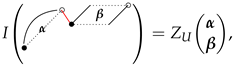
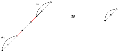
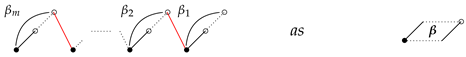
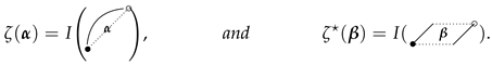
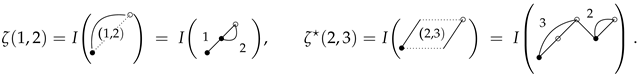
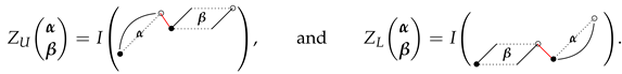
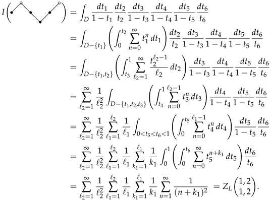
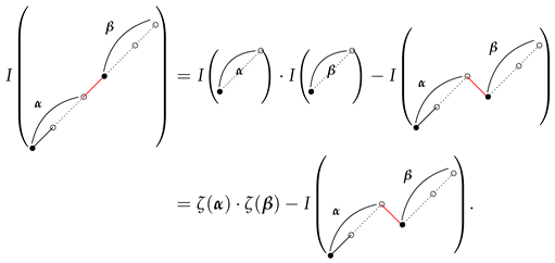
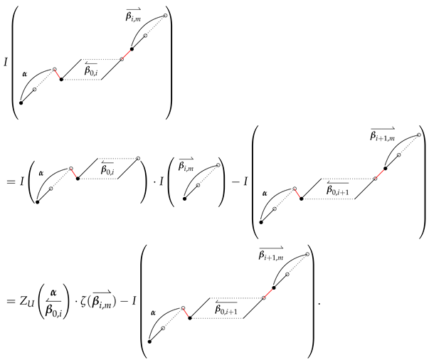
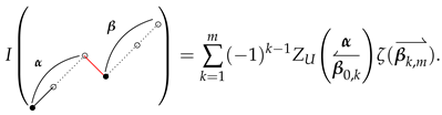
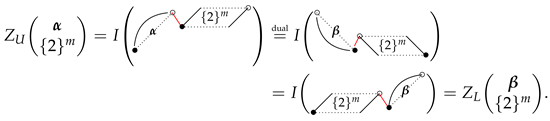
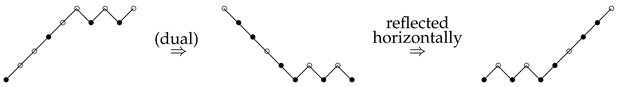
2—Yamamoto’s integral. Since the duality of the Euler sums is represented by $u_i=1-t_i$ in its Drinfel’d iterated integral, the corresponding 2-poset Hasse diagram appears as a vertical reflection, with ∘ and • interchanged.

We explain it by an example with $Z_U{\left(\begin{array}{c}3,3\\ 2,2\end{array}\right)}^{\#}=Z_L\left(\begin{array}{c}1,2,1,2\\ 2,2\end{array}\right)$.

Method 

3—Expressions by MZVs and MZSVs. We use Equations (13) and (11), we know that

$$\begin{array}{cc}\hfill Z_U\left(\begin{array}{c}\mathit{\alpha }\\ {\left\{2\right\}}^n\end{array}\right)& =\sum _{a+b=n}{(-1)}^a\zeta (\mathit{\alpha },{\left\{2\right\}}^a){\zeta }^{★}\left({\left\{2\right\}}^b\right),\hfill \\ \hfill Z_L\left(\begin{array}{c}\mathit{\beta }\\ {\left\{2\right\}}^n\end{array}\right)& =\sum _{a+b=n}{(-1)}^a\zeta ({\left\{2\right\}}^a,\mathit{\beta }){\zeta }^{★}\left({\left\{2\right\}}^b\right).\hfill \end{array}$$

Since $\zeta {\left(\mathit{\alpha }\right)}^{♯}=\zeta \left(\mathit{\beta }\right)$, this implies that $\zeta {(\mathit{\alpha },{\left\{2\right\}}^a)}^{♯}=\zeta ({\left\{2\right\}}^a,\mathit{\beta })$. Thus, we have

$$\begin{array}{cc}\hfill Z_U\left(\begin{array}{c}\mathit{\alpha }\\ {\left\{2\right\}}^n\end{array}\right)& =\sum _{a+b}\zeta (\mathit{\alpha },{\left\{2\right\}}^a){\zeta }^{★}\left({\left\{2\right\}}^b\right)\hfill \\ \hfill & =\sum _{a+b}\zeta ({\left\{2\right\}}^a,\mathit{\beta }){\zeta }^{★}\left({\left\{2\right\}}^b\right)=Z_L\left(\begin{array}{c}\mathit{\beta }\\ {\left\{2\right\}}^n\end{array}\right).\hfill \end{array}$$

Next, we proceed to prove the second equation of Theorem 2.

Using Equation (16), we know that

$$Z_B\left(\begin{array}{c}\mathit{\alpha }\\ {\left\{2\right\}}^m\end{array}\right)=\sum _{a+b+c=m}{(-1)}^{a+b}\zeta ({\left\{2\right\}}^a,\mathit{\alpha },{\left\{2\right\}}^b){\zeta }^{★}\left({\left\{2\right\}}^c\right).$$

It is easy to see that $\zeta {({\left\{2\right\}}^a,\mathit{\alpha },{\left\{2\right\}}^b)}^{♯}=\zeta ({\left\{2\right\}}^b,\mathit{\beta },{\left\{2\right\}}^a)$, we have

$$\begin{array}{cc}\hfill Z_B\left(\begin{array}{c}\mathit{\alpha }\\ {\left\{2\right\}}^n\end{array}\right)& =\sum _{a+b+c=n}{(-1)}^{a+b}\zeta ({\left\{2\right\}}^a,\mathit{\alpha },{\left\{2\right\}}^b){\zeta }^{★}\left({\left\{2\right\}}^c\right)\hfill \\ \hfill & =\sum _{a+b+c=n}{(-1)}^{a+b}\zeta ({\left\{2\right\}}^b,\mathit{\beta },{\left\{2\right\}}^a){\zeta }^{★}\left({\left\{2\right\}}^c\right)=Z_B\left(\begin{array}{c}\mathit{\beta }\\ {\left\{2\right\}}^n\end{array}\right).\hfill \end{array}$$

Therefore, the function $Z_B$ satisfies second equation. We complete the proof.

Nakasuji, Ohno (Theorem 4.4, [17]) use Schur multiple zeta functions to give a more general duality theorem. However, our particular duality forms are founded by the classical generating functions, or the new Yamamoto’s integral.

Since $\zeta {\left(k\right)}^{♯}=\zeta ({\left\{1\right\}}^{k-2},2)$, for $k\ge 2$. Then, for any nonnegative integer n, we have

$$\begin{array}{cc}\hfill \zeta (2n+k)& =Z_B\left(\begin{array}{c}k\\ {\left\{2\right\}}^n\end{array}\right)=Z_B\left(\begin{array}{c}{\left\{1\right\}}^{k-2},2\\ {\left\{2\right\}}^n\end{array}\right)\hfill \\ \hfill & =\sum _{a+b+c=n}{(-1)}^{a+b}\zeta ({\left\{2\right\}}^a,{\left\{1\right\}}^{k-2},{\left\{2\right\}}^{b+1}){\zeta }^{★}\left({\left\{2\right\}}^c\right).\hfill \end{array}$$

Let $k=2$, we have the following weighted sum formula:

$$\zeta (2n+2)=\sum _{a+b=n}{(-1)}^b(b+1)\zeta \left({\left\{2\right\}}^{b+1}\right){\zeta }^{★}\left({\left\{2\right\}}^a\right).$$

(22)

5. Theorem 3 and Some More Formulas

In this last section, we will start by providing the proof of Theorem 3, and then we will discuss some applications.

Proof of Theorem 3.

Let

$$G\left(x\right)=\sum _{p=0}^{\infty }{\zeta }^{★}({\left\{2\right\}}^p,{\left\{1\right\}}^r,{\left\{2\right\}}^q)x^{2p}$$

be the generating function of ${\zeta }^{★}({\left\{2\right\}}^p,{\left\{1\right\}}^r,{\left\{2\right\}}^q)x^{2p}$. Thus,

$$\begin{array}{cc}\hfill G\left(x\right)& =\sum _{1\le k_1\le k_2\le \cdots \le k_{q+r}}{\displaystyle \frac{{\prod }_{1\le j\le k_1}{\left(1-\frac{x^2}{j^2}\right)}^{-1}}{k_1{k}_2\cdots k_r{k}_{r+1}^2{k}_{r+2}^2\cdots k_{q+r}^2}}\hfill \\ \hfill & ={\displaystyle \frac{\pi x}{sin\left(\pi x\right)}}\sum _{1\le k_1\le k_2\le \cdots \le k_{q+r}}{\displaystyle \frac{{\prod }_{j>k_1}\left(1-\frac{x^2}{j^2}\right)}{k_1{k}_2\cdots k_r{k}_{r+1}^2{k}_{r+2}^2\cdots k_{q+r}^2}}.\hfill \end{array}$$

We represent the above summation as

$${\zeta }^{★}({\left\{1\right\}}^r,{\left\{2\right\}}^q)+\sum _{n=1}^{\infty }{(-1)}^n{Z}_L\left(\begin{array}{c}1,{\left\{2\right\}}^n\\ {\left\{1\right\}}^{r-1},{\left\{2\right\}}^q\end{array}\right)x^{2n}.$$

By convolution, we have

$$\begin{array}{cc}\hfill G\left(x\right)& =\sum _{n=0}^{\infty }{\zeta }^{★}\left({\left\{2\right\}}^n\right){\zeta }^{★}({\left\{1\right\}}^r,{\left\{2\right\}}^q)x^{2n}\hfill \\ \hfill & +\sum _{p=1}^{\infty }\left(\sum _{{\displaystyle \genfrac{}{}{0pt}{}{m+n=p}{m\ge 1}}}{(-1)}^m{\zeta }^{★}\left({\left\{2\right\}}^n\right)Z_L\left(\begin{array}{c}1,{\left\{2\right\}}^m\\ {\left\{1\right\}}^{r-1},{\left\{2\right\}}^q\end{array}\right)\right)x^{2p}.\hfill \end{array}$$

Comparing the coefficient of $x^{2p}$, for $p\ge 1$, we have

$$\begin{array}{cc}\hfill {\zeta }^{★}({\left\{2\right\}}^p,{\left\{1\right\}}^r,{\left\{2\right\}}^q)& ={\zeta }^{★}\left({\left\{2\right\}}^p\right){\zeta }^{★}({\left\{1\right\}}^r,{\left\{2\right\}}^q)\hfill \\ \hfill & +\sum _{m+n=p-1}{(-1)}^{m+1}{\zeta }^{★}\left({\left\{2\right\}}^n\right)Z_L\left(\begin{array}{c}1,{\left\{2\right\}}^{m+1}\\ {\left\{1\right\}}^{r-1},{\left\{2\right\}}^q\end{array}\right).\hfill \end{array}$$

(23)

We use Equation (7) to the function $Z_L$, this gives

$$\begin{array}{cc}\hfill Z_L\left(\begin{array}{c}1,{\left\{2\right\}}^{m+1}\\ {\left\{1\right\}}^{r-1},{\left\{2\right\}}^q\end{array}\right)& ={(-1)}^{r-1}{Z}_L\left(\begin{array}{c}{\left\{1\right\}}^r,{\left\{2\right\}}^{m+1}\\ {\left\{2\right\}}^q\end{array}\right)\hfill \\ \hfill & +\sum _{a+b=r-2}{(-1)}^a\zeta ({\left\{1\right\}}^{a+1},{\left\{2\right\}}^{m+1}){\zeta }^{★}({\left\{1\right\}}^{b+1},{\left\{2\right\}}^q).\hfill \end{array}$$

It is clear that $\zeta {({\left\{1\right\}}^{a+1},{\left\{2\right\}}^{m+1})}^{♯}=\zeta ({\left\{2\right\}}^m,a+3)$, and we apply the dual theorem to transform

$$Z_L\left(\begin{array}{c}{\left\{1\right\}}^r,{\left\{2\right\}}^{m+1}\\ {\left\{2\right\}}^q\end{array}\right)=Z_U\left(\begin{array}{c}{\left\{2\right\}}^m,r+2\\ {\left\{2\right\}}^q\end{array}\right)$$

then we obtain

$$\begin{array}{cc}\hfill Z_L\left(\begin{array}{c}1,{\left\{2\right\}}^{m+1}\\ {\left\{1\right\}}^{r-1},{\left\{2\right\}}^q\end{array}\right)& ={(-1)}^{r-1}{Z}_U\left(\begin{array}{c}{\left\{2\right\}}^m,r+2\\ {\left\{2\right\}}^q\end{array}\right)\hfill \\ \hfill & +\sum _{a+b=r-2}{(-1)}^a\zeta ({\left\{2\right\}}^m,a+3){\zeta }^{★}({\left\{1\right\}}^{b+1},{\left\{2\right\}}^q).\hfill \end{array}$$

The summation in Equation (23) becomes

$$\begin{array}{cc}\hfill & \sum _{m+n=p-1}{(-1)}^{m+r}{\zeta }^{★}\left({\left\{2\right\}}^n\right)Z_U\left(\begin{array}{c}{\left\{2\right\}}^m,r+2\\ {\left\{2\right\}}^q\end{array}\right)\hfill \\ \hfill & +\sum _{m+n=p-1}\sum _{a+b=r-2}{(-1)}^{m+a+1}{\zeta }^{★}\left({\left\{2\right\}}^n\right)\zeta ({\left\{2\right\}}^m,a+3){\zeta }^{★}({\left\{1\right\}}^{b+1},{\left\{2\right\}}^q).\hfill \end{array}$$

The second summation of the above formula can be simplified by using Equation (9)

$$\sum _{m+n=p-1}{(-1)}^m{\zeta }^{★}\left({\left\{2\right\}}^n\right)\zeta ({\left\{2\right\}}^m,a+3)={\zeta }^{★}(a+3,{\left\{2\right\}}^{p-1}).$$

We will obtain

$$\sum _{a+b=r-2}{(-1)}^{a+1}{\zeta }^{★}(a+3,{\left\{2\right\}}^{p-1}){\zeta }^{★}({\left\{1\right\}}^{b+1},{\left\{2\right\}}^q).$$

It remains to treat the summation

$$\sum _{m+n=p-1}{(-1)}^{m+r}{\zeta }^{★}\left({\left\{2\right\}}^n\right)Z_U\left(\begin{array}{c}{\left\{2\right\}}^m,r+2\\ {\left\{2\right\}}^q\end{array}\right).$$

We apply Equation (19) with $\mathit{\alpha }=\left({\left\{2\right\}}^q\right)$, $\theta =r+2$, and $\mathit{\beta }=\left({\left\{2\right\}}^{p-1}\right)$, then the above summation is equal to

$${(-1)}^r{\zeta }^{★}({\left\{2\right\}}^q,r+2,{\left\{2\right\}}^{p-1}).$$

Therefore, Equation (23) becomes

$$\begin{array}{cc}\hfill {\zeta }^{★}({\left\{2\right\}}^p,{\left\{1\right\}}^r,{\left\{2\right\}}^q)& ={\zeta }^{★}\left({\left\{2\right\}}^p\right){\zeta }^{★}({\left\{1\right\}}^r,{\left\{2\right\}}^q)+{(-1)}^r\zeta ({\left\{2\right\}}^q,r+2,{\left\{2\right\}}^{p-1})\hfill \\ \hfill & +\sum _{a+b=r-2}{(-1)}^{a+1}{\zeta }^{★}(a+3,{\left\{2\right\}}^{p-1}){\zeta }^{★}({\left\{1\right\}}^{b+1},{\left\{2\right\}}^q)\hfill \\ \hfill & ={(-1)}^r{\zeta }^{★}({\left\{2\right\}}^q,r+2,{\left\{2\right\}}^{p-1})\hfill \\ \hfill & +\sum _{a+b=r-1}{(-1)}^a{\zeta }^{★}(a+2,{\left\{2\right\}}^{p-1}){\zeta }^{★}({\left\{1\right\}}^{b+1},{\left\{2\right\}}^q).\hfill \end{array}$$

This finishes our work. □

It is well-known that (ref. [18]) ${\zeta }^{★}(1,{\left\{2\right\}}^q)=2\zeta (2q+1)$, and we leverage Zagier’s formula (ref. [16]) to compute ${\zeta }^{★}({\left\{2\right\}}^q,3,{\left\{2\right\}}^{p-1})$:

$${\zeta }^{★}({\left\{2\right\}}^q,3,{\left\{2\right\}}^{p-1})=-2\sum _{k=1}^{p+q}\left[\left({\displaystyle \genfrac{}{}{0pt}{}{2k}{2q}}\right)-{\delta }_{k,q}-\left(1-{\displaystyle \frac{1}{2^{2k}}}\right)\left({\displaystyle \genfrac{}{}{0pt}{}{2k}{2p-1}}\right)\right]{\zeta }^{★}\left({\left\{2\right\}}^{p+q-k}\right)\zeta (2k+1).$$

By substituting $r=1$ in Equation (3), we obtain an evaluation of ${\zeta }^{★}({\left\{2\right\}}^p,1,{\left\{2\right\}}^q)$, for any positive integers p and q (Theorem 1.6, [13]):

$${\zeta }^{★}({\left\{2\right\}}^p,1,{\left\{2\right\}}^q)=2\sum _{k=1}^{p+q}\left[\left({\displaystyle \genfrac{}{}{0pt}{}{2k}{2q}}\right)-\left(1-{\displaystyle \frac{1}{2^{2k}}}\right)\left({\displaystyle \genfrac{}{}{0pt}{}{2k}{2p-1}}\right)\right]{\zeta }^{★}\left({\left\{2\right\}}^{p+q-k}\right)\zeta (2k+1).$$

On the other hand, if we apply $p=q=1$ in Equation (3), then

$$\sum _{a+b=r}{(-1)}^a(b+1)\zeta (a+2)\zeta (b+2)={\zeta }^{★}(2,{\left\{1\right\}}^r,2)+{(-1)}^r\zeta (r+2,2),$$

for any nonnegative integer r, by using the fact (ref. [5]) ${\zeta }^{★}({\left\{1\right\}}^{b+1},2)=(b+2)\zeta (b+3)$.

References

1. Hoffman, M.E. Multiple harmonic series. Pac. J. Math. 1992, 152, 275–290. [Google Scholar] [CrossRef]
2. Ohno, Y. Sum relations for multiple zeta values. In Zeta Functions, Topology and Quantum Physics, Developments in Mathematics; Aoki, T., Kanemitsu, S., Nakahara, M., Ohno, Y., Eds.; Springer: Boston, MA, USA, 2005; Volume 14, pp. 131–144. [Google Scholar]
3. Zagier, D. Values of zeta functions and their applications. In First European Congress of Mathematics Paris; Birkhäuser: Baesl, Switzerland, 1994; Volume II, pp. 497–512. [Google Scholar]
4. Chen, K.-W. Generalized harmonic numbers and Euler sums. Int. J. Number Theory 2017, 13, 513–528. [Google Scholar] [CrossRef]
5. Chen, K.-W.; Eie, M. On three general forms of multiple zeta(-star) values. Expo. Math. 2023, 41, 299–315. [Google Scholar] [CrossRef]
6. Chen, K.-W.; Chung, C.-L.; Eie, M. Sum formulas and duality theorems of multiple zeta values. J. Number Theory 2016, 158, 33–53. [Google Scholar] [CrossRef]
7. Yamamoto, S. Multiple zeta-star values and multiple integrals. RIMS Kôky r ̂ oku Bessatsu 2017, B68, 3–14. [Google Scholar]
8. Kaneko, M.; Yamamoto, S. A new integral-series identity of multiple zeta values and regularizations. Sel. Math. New Ser. 2018, 24, 2499–2521. [Google Scholar] [CrossRef]
9. Hirose, M.; Murahara, H.; Ono, M. On variants of symmetric multiple zeta-star values and the cyclic sum formula. Ramanujan J. 2021, 56, 467–489. [Google Scholar] [CrossRef]
10. Yamamoto, S. Integrals associated with 2-posets and applications to multiple zeta values. RIMS Kôky r ̂ oku Bessatsu 2020, B83, 27–46. [Google Scholar]
11. Nakasuji, M.; Phuksuwan, O.; Yamasaki, Y. On Schur multiple zeta functions: A combinatoric generalization of multiple zeta functions. Adv. Math. 2018, 333, 570–619. [Google Scholar] [CrossRef]
12. Nakasuji, M.; Takeda, W. Shuffle product formula of the Schur multiple zeta values of hook type. arXiv 2022, arXiv:2202.01402v2. [Google Scholar]
13. Tasaka, K.; Yamamoto, S. On some multiple zeta-star values of one-two-three indices. Inter. J. Number Theory 2013, 9, 1171–1184. [Google Scholar] [CrossRef]
14. Xu, C. Evaluations of nonlinear Euler sums of weight ten. Appl. Math. Comput. 2019, 346, 594–611. [Google Scholar] [CrossRef]
15. Ohno, Y. A generalization of the duality and sum formulas on the multiple zeta values. J. Number Theory 1999, 74, 39–43. [Google Scholar] [CrossRef]
16. Zagier, D. Evaluation of the multiple zeta value ζ(2,,2,3,2,,2). Ann. Math. 2012, 175, 977–1000. [Google Scholar] [CrossRef]
17. Nakasuji, M.; Ohno, Y. Duality formula and its generalization for Schur multiple zeta functions. arXiv 2019, arXiv:2109.14362v1. [Google Scholar]
18. Zlobin, S.A. Generating functions for the values of a multiple zeta function. Vestnik Moskov. Univ. Ser. 1 Mat. Mekh. 2005, 2, 55–59. [Google Scholar]
Disclaimer/Publisher’s Note: The statements, opinions and data contained in all publications are solely those of the individual author(s) and contributor(s) and not of MDPI and/or the editor(s). MDPI and/or the editor(s) disclaim responsibility for any injury to people or property resulting from any ideas, methods, instructions or products referred to in the content.