Dynamics of a Price Adjustment Model with Distributed Delay

Abstract

This paper deals with the stability and occurrence of Hopf bifurcation of a distributed delay differential cobweb model using the chain trick technique. This is a generalized form of the fixed delay cobweb model to which it is compared using the same parameter values. The results from the delay distribution showed that whenever less weight $(\gamma =0.146)$ is put on past prices, the current equilibrium price is adjusted upwards while the reverse is observed when a higher weight $(\gamma =0.186)$ is put on the previous price. It is also observed that if the initial price is set below/above the equilibrium price, the price adjustment either affects the consumers or benefits the suppliers. However, the fixed delay cobweb model does not display the consumers or suppliers benefits of the price dynamics in either direction. These are unique, underlying patterns in price dynamics discovered when using a distributed delay model compared to traditional fixed delay cobweb models. Furthermore, our model challenges the traditional cobweb model’s requirement for divergence, as it is based on the weight assigned to past prices rather than the relationship between the elasticities of supply and demand, which is the determining factor in the classical model. Based on these insights, we recommend that future price adjustment models incorporate distributed delays, as they reveal more intricate price dynamics and provide a more comprehensive understanding of market behavior than fixed delay models.

1. Introduction

The dynamics of economic markets reveal an inverse relationship between the price of a commodity and the quantity demanded, and a direct relationship between the price and the quantity supplied [1]. Thus, as a commodity’s price rises, the demand decreases because fewer people can afford it [1,2]. This fluctuation in price, driven by the interaction between the demand function of the current price and the supply function of the expected price, is most effectively described by the cobweb model [3]. Various forms of this model have been applied in research, such as Nerlove’s study of adaptive expectations [4] and Muth’s work on rational expectations [5], both investigating the theory of price movements. Hommes [5,6] also examined the chaotic dynamics and bifurcations in cobweb model solutions, while Gaffney and Pearce [7] explored the model’s dynamics using nonlinear forms. The classical cobweb model assumes that the supply function reacts to prices with a one-period lag [8], while demand depends on the current price. The time gap between supply and demand, often linked to price volatility [9,10], has led to the increasing use of delay differential equations in modeling price adjustments.

Delay parameters enrich the dynamics of price adjustment models [11] by reflecting suppliers’ past decisions. For instance, Ma et al. [12] applied a cobweb model with delayed feedback to control chaos in the price system. Matsumoto et al. [13] and Gori et al. [14], respectively, investigated the asymptotic behavior and Hopf bifurcation in cobweb models with time delays. The time delay parameter has been found to play a crucial role even in models with varying price expectations [15]. According to Gori et al. [16], quasi-periodic oscillations occur when the time delay parameter becomes very large for a sufficiently low elasticity of demand. Additionally, Matsumoto and Nakayama [17] introduced two-time delays in a cobweb model, revealing a winding stability switching curve.

Anokye et al. [18] recently used a new method to find a unique solution to the following delay differential cobweb model via the Lambert W-function without considering any complex branches,

$$\dot{p}\left(t\right)=\gamma \left[\alpha -\lambda -\beta p\left(t\right)-\delta p(t-\tau )\right],$$

(1)

$$p\left(t\right)=p_0\left(t\right)-\tau \le t\le 0$$

where the function $p\left(t\right)$ represents the price at time t, and the positive parameters $\alpha ,\beta ,\gamma ,\delta$ and $\lambda$ are defined as the demand intercept (to ensure that there is demand for the commodity even at the lowest price), elasticity of demand, market adjustment coefficient, elasticity of supply, and supply intercept, respectively. According to the rules governing the cobweb model, these parameters assume that $\alpha >\lambda$, and for the condition of price convergence, $\beta >\delta$; otherwise, $\beta <\delta$. Additionally, $\tau >0$ represents a time delay. The model operates using only the previous price (naive price expectation) to make decisions [19] and does not incorporate any exogenous factors affecting price. Equation (1) has a unique positive equilibrium

$$p_{\ast }={\displaystyle \frac{\alpha -\lambda }{\beta +\delta }},$$

obtained by setting $\dot{p}\left(t\right)=0$ and $p(t-\tau )=p\left(t\right)=p_{\ast }$ for all $t.$

There are various forms of delay-related models used in the modeling of dynamical systems. One such form is distributed delay equations, which are employed to model delayed systems where the duration of the delay is uncertain [19]. Many researchers focus on models where the delay can change arbitrarily, as it is often realistic for delays in a system to vary over time. To capture this variability, distributed delay equations are used, as the delayed terms in these models represent an expectation [19]. A more general and realistic [20] approach for modeling processes that might exhibit intrinsic stochasticity on a smaller scale, but manifest this randomness at a larger scale, is through the use of distributed delay models. For example, certain physical systems, such as hematopoiesis and lactose operon dynamics in biological systems, show intrinsic stochastic time delay behavior, and these phenomena have been modeled using distributed time delay equations [21,22,23,24,25]. Empirical studies have also shown that the placement of delay terms within a model can significantly influence the system’s behavior as the average time delay increases [26]. Additionally, it has been discovered that when time delays approach the same scale as pattern formation, they can alter the system’s overall dynamics [26].Therefore, evaluating how temporal delays impact dynamical system models is crucial.

Since much of the literature on cobweb models has focused on fixed delay models [19,20,27], and these models often oversimplify or overlook critical price dynamics [26], as fixed time delays are seen as a simplification of the underlying process in dynamical systems, this study considers a distributed delay model. Distributed delay models are better suited to capturing complex price behaviors because they account for varying time lags in the supply function and introduce heterogeneity [20,22], making the models more realistic. Moreover, the dynamics of cobweb models with distributed delays have not received significant research attention, despite distributed delays being more general than discrete delays.

In this paper, we generalize Equation (1) by incorporating distributed delays using the chain trick method. The aim is to assess whether the results from the fixed delay model remain consistent across different delay distributions or if they are sensitive to changes in the delay structure. The model for the study is expressed by

$$\dot{p}\left(t\right)=\gamma \left[\alpha -\lambda -\beta p\left(t\right)-\delta {\int }_{-\infty }^{t}p\left(r\right)g(t-r)dr\right],$$

(2)

$$p\left(t\right)=p_0\left(t\right)-\tau \le t\le 0$$

where the delay kernel $g(·)$ is a gamma distribution, i.e.,

$$g\left(t\right)={\left({\displaystyle \frac{m}{T}}\right)}^m{\displaystyle \frac{t^{m-1}{e}^{-\frac{m}{T}t}}{(m-1)!}}.$$

(3)

Here, m is a positive integer and T is a positive real, which corresponds to the average length of delay. Notice that the distribution function approaches the Dirac distribution as $T\to 0$, so that one recovers the time delay case. Hence, discrete delay may be seen as a limiting case of distributed delay. Thus, the fixed delay model (1) is now modified as a distributed delay model as shown above so that we can investigate the effect of the distributed time delay and the weight function (of the past price) on the current price. It should be noted that the assumptions mentioned in model (1) are also relevant to model (2).

The rest of the paper is structured as follows: Section 2 discusses the local stability analysis, stability switch and bifurcation analysis, and the existence and uniqueness of the solution of Equation (2). In Section 3, detailed numerical solutions and stability analyses are performed by comparing model (2) with model (1) given in the literature. Section 4 provides the findings and conclusions derived from the analyses of the two models.

2. Materials and Methods

2.1. Stability Analysis of Solution

To examine the local dynamic behavior of the integro-differential equation system (2) at the equilibrium point $p_{\ast }$, we use the translation $z=p-p_{\ast }$ and consider the linearization of (2) at the origin. This may be written as

$$\dot{z}\left(t\right)=-\beta \gamma z\left(t\right)-\delta \gamma {\int }_{-\infty }^{t}z\left(r\right)g(t-r)dr.$$

(4)

By employing the procedures delineated by Miller [19], we can determine the characteristic equation of (4) by looking for solutions of the form $z\left(t\right)=z\left(0\right)e^{\mu t},\mu \in \mathbb{C}$. Substituting this last expression into (4) yields

$$\mu +\beta \gamma +\delta \gamma {\int }_{-\infty }^t{e}^{-\mu (t-r)}g(t-r)dr=0.$$

(5)

Since

$$\begin{array}{ccc}\hfill {\int }_{-\infty }^t{e}^{-\mu (t-r)}g(t-r)dr& =& {\int }_0^{+\infty }{e}^{-\mu v}g\left(v\right)dv\hfill \\ & =& {\left({\displaystyle \frac{m}{T}}\right)}^m{\displaystyle \frac{1}{(m-1)!}}{\int }_0^{+\infty }{v}^{m-1}{e}^{-\left({\displaystyle \frac{m}{T}}+\mu \right)v}dv={\left(1+{\displaystyle \frac{\mu T}{m}}\right)}^{-m}.\hfill \end{array}$$

the characteristic Equation (5) assumes the form

$$(\mu +\beta \gamma ){\left(1+{\displaystyle \frac{\mu T}{m}}\right)}^m+\delta \gamma =0,$$

(6)

which is a polynomial in $\mu$ of degree $m+1$. It is difficult to obtain a general solution of (6). Thus, to gain insight into the dynamic characteristics of our model, we confine the attention to the special cases $m=1$ and $m=2$, which are called weak delay kernel and strong delay kernel, respectively. The weak kernel posits that the importance of past events decreases exponentially as one goes deeper into the past, whereas the strong kernel asserts that a specific instant in the past holds greater significance than all others.

• Case $m=1$. By substituting $m=1$ into (6), we obtain the quadratic characteristic equation

  $${\mu }^2+b_1\left(T\right)\mu +b_2\left(T\right)=0,$$

  (7)

  where

  $$b_1\left(T\right)=\beta \gamma +{\displaystyle \frac{1}{T}}>0,b_2\left(T\right)={\displaystyle \frac{\gamma (\beta +\delta )}{T}}>0.$$

  The local asymptotical stability of the model is guaranteed if both roots of Equation (7) have negative real parts. According to the Routh–Hurwitz criterion, this holds true if and only if $b_1\left(T\right)>0$ and $b_2\left(T\right)>0.$ We, therefore, have the following result.

Proposition 1.

The equilibrium point $p_{\ast }$ of (2) is locally asympotically stable for all $T>0$.

• Case $m=2$. In this case, the characteristic Equation (6) takes the form

  $${\mu }^3+b_1\left(T\right){\mu }^2+b_2\left(T\right)\mu +b_3\left(T\right)=0,$$

  (8)

  where

  $$b_1\left(T\right)=\beta \gamma +{\displaystyle \frac{4}{T}}>0,b_2\left(T\right)={\displaystyle \frac{4}{T}}\left(\beta \gamma +{\displaystyle \frac{1}{T}}\right)>0,b_3\left(T\right)={\displaystyle \frac{4\gamma (\beta +\delta )}{T^2}}>0.$$

  By the Routh–Hurwitz criterion, the equilibrium is locally asymptotically stable if and only if $b_1\left(T\right)>0,b_3\left(T\right)>0$ and $b_1\left(T\right)b_2\left(T\right)-b_3\left(T\right)>0$. Since the coefficients of (8) are all positive, the stability condition is validated if

  $${\beta }^2{\gamma }^2{T}^2-\gamma \left(\delta -4\beta \right)T+4>0.$$

  (9)

Proposition 2.

(1)

Let $\beta <\delta <8\beta$. The equilibrium point $p_{\ast }$ of (2) is locally asympotically stable for all $T>0$.

(2)

Let $\delta =8\beta$. The equilibrium point $p_{\ast }$ of (2) is locally asympotically stable for all $T\ne T_0$, where

$$T_0={\displaystyle \frac{1}{4{\beta }^2}}>0.$$

(3)

Let $\delta >8\beta$. The equilibrium point $p_{\ast }$ of (2) is locally asympotically stable if $T<T_1$ and $T>T_2$ and unstable if $T_1<T<T_2$, where

$$T_1={\displaystyle \frac{\delta -4\beta -\sqrt{\delta (\delta -8\beta )}}{2{\beta }^2\gamma }}>0,T_2={\displaystyle \frac{\delta -4\beta +\sqrt{\delta (\delta -8\beta )}}{2{\beta }^2\gamma }}>0.$$

Proof. 

If $4\beta -\delta \ge 0,$ then (9) is clearly satisfied. If $4\beta -\delta <0,$ then the statement follows from ${\gamma }^2\delta \left(\delta -8\beta \right)$ being the discriminant of our inequality and recalling the assumption $\delta >\beta .$  □

2.2. Stability Switches and Bifurcation

The next question that naturally arises is on the dynamics when the equilibrium loses stability. Hence, we go back to the characteristic Equation (8) evaluated at $T=T_{\ast }$, where $T_{\ast }\in \left\{T_1,T_2\right\}.$ Since $b_1\left(T_{\ast }\right)b_2\left(T_{\ast }\right)-b_3\left(T_{\ast }\right)=0,$ by replacing $b_3\left(T_{\ast }\right)$ with $b_1\left(T_{\ast }\right)b_2\left(T_{\ast }\right)$, we are able to factor (8) as

$$\left[\mu +b_1\left(T_{\ast }\right)\right]\left[{\mu }^2+b_2\left(T_{\ast }\right)\right]=0,$$

that can be explicitly solved for $\mu$. One of the three roots is real and negative, whereas the other two are pure imaginary

$${\mu }_1=-b_1\left(T_{\ast }\right),{\mu }_{2,3}=\pm i\sqrt{b_2\left(T_{\ast }\right)}=\pm i{\omega }_{\ast }.$$

In order to apply the Hopf bifurcation theorem, we need to show that the real parts of the complex roots are sensitive to a change in the bifurcation parameter $T.$ Suppose that $\mu$ is a function of T. Taking the derivative of the characteristic Equation (8) with respect to $T,$ we have

$${\displaystyle \frac{d\mu }{dT}}=-{\displaystyle \frac{b_1^{\prime }\left(T\right){\mu }^2+b_2^{\prime }\left(T\right)\mu +b_3^{\prime }\left(T\right)}{3{\mu }^2+2b_1\left(T\right)\mu +b_2\left(T\right)}},$$

(10)

where

$$b_1^{\prime }\left(T\right)=-{\displaystyle \frac{4}{T^2}},b_2^{\prime }\left(T\right)=-{\displaystyle \frac{4}{T^2}}\left(\beta \gamma +{\displaystyle \frac{2}{T}}\right),b_3^{\prime }\left(T\right)=-{\displaystyle \frac{8\gamma (\beta +\delta )}{T^3}}.$$

Plugging $\mu =i{\omega }_{\ast }$ in (10), and arranging terms yields

$$Re{\left({\displaystyle \frac{d\mu }{dT}}\right)}_{\mu =i{\omega }_{\ast }}={\displaystyle \frac{2\left[{\beta }^2{\gamma }^2{T}_{\ast }^2-2\gamma \left(\delta -4\beta \right)T_{\ast }+12\right]}{\left(\beta \gamma T_{\ast }+10\right)\left(\beta \gamma T_{\ast }+2\right)T_{\ast }^2}}.$$

(11)

Plugging ${\beta }^2{\gamma }^2{T}_{\ast }^2-\gamma \left(\delta -4\beta \right)T_{\ast }+4=0$ into the numerator of (11), we obtain

$$sign\left[Re{\left({\displaystyle \frac{d\mu }{dT}}\right)}_{\mu =i{\omega }_{\ast }}\right]=sign\left\{-\gamma \left(\delta -4\beta \right)T_{\ast }+8\right\}.$$

For $T_{\ast }=T_1,$ we derive

$$sign\left\{-\gamma \left(\delta -4\beta \right)T_1+8\right\}>0.$$

Notice, one has

$$-\gamma \left(\delta -4\beta \right)T_1+8={\displaystyle \frac{-\delta \left(\delta -8\beta \right)+\left(\delta -4\beta \right)\sqrt{\delta (\delta -8\beta )}}{2{\beta }^2}},$$

where the numerator is positive being $-\delta \left(\delta -8\beta \right)+\left(\delta -4\beta \right)\sqrt{{\delta }^2-8\beta \delta }>0$ if and only if $16{\beta }^2>0.$ On the other hand, for $T_{\ast }=T_2,$ we find

$$sign\left\{-\gamma \left(\delta -4\beta \right)T_2+8\right\}<0.$$

Notice, one has

$$-\gamma \left(\delta -4\beta \right)T_2+8={\displaystyle \frac{-\delta \left(\delta -8\beta \right)-\left(\delta -4\beta \right)\sqrt{\delta (\delta -8\beta )}}{2{\beta }^2}},$$

with the assumption $\delta -8\beta >0$ implying the numerator to be negative. In conclusion, crossing of the imaginary axis is from left to right as T increases to a certain critical value $T_1$ (stability loss), and crossing from right to left occurs at a certain value $T_2$ (stability gain). Our analysis is summarized in the following theorem.

Theorem 1.

Let $\delta >8\beta$. The equilibrium point $p_{\ast }$ of (2) undergoes a Hopf bifurcation for $T=T_1$ and $T=T_2$.

2.3. Existence and Uniqueness of Solution

We use the Banach fixed point theorem to determine the existence and uniqueness of the model. We set $Tz=z$

$$\dot{z}\left(t\right)=-\beta \gamma z\left(t\right)-\delta \gamma {\int }_{-\infty }^{t}z\left(r\right)g(t-\tau )dr.$$

(12)

Then, we express (12) as

$$Tz={\displaystyle \frac{1}{\beta \gamma }}\left[\dot{z}\left(t\right)+\sigma \gamma {\int }_{-\infty }^{b}z\left(r\right)g(t-\tau )dr\right].$$

(13)

Since $g(t-\tau )$ is continuous, we have that $\left|g\right(t-\tau \left)\right|\le k$. For the uniqueness of the solution,

$$\begin{array}{ccc}\hfill T{z}_1\left(t\right)-T{z}_2\left(t\right)& =& {\displaystyle \frac{1}{\beta \gamma }}\left|\sigma \gamma \right|{\int }_{-\infty }^{t}g(t-\tau )[z_1\left(r\right)-z_2\left(r\right)]dr\hfill \\ & \le & {\displaystyle \frac{1}{\beta \gamma }}\left|\sigma \gamma \right|c|z_1-z_2|{\int }_{\infty }^{t}dr\hfill \\ & =& {\displaystyle \frac{1}{\beta \gamma }}\sigma \gamma \left|c(t-a)\right||z_1-z_2|.\hfill \end{array}$$

By induction,

$$\left|T^m{z}_1-T^m{z}_2\right|\le {\left({\displaystyle \frac{1}{\beta \gamma }}\right)}^m{\left|\sigma \gamma \right|}^m{c}^m|{\displaystyle \frac{{(t-a)}^m}{m!}}\left|z_1-z_2\right|,$$

for $m=1$, we obtain

$$\left|T{z}_1-T{z}_2\right|\le \left|{\displaystyle \frac{1}{{\beta }^{\gamma }}}\right|\left|\sigma \gamma \right|c(t-a)\left|z_1-z_2\right|.$$

(14)

Assuming that (14) is true for any m, we obtain

$$\begin{array}{ccc}\hfill \left|T^{m+1}{z}_1-T^{m+1}{z}_2\right|& =& \left|{\displaystyle \frac{1}{\beta \gamma }}\right||\delta \gamma \mid {\int }_{-\infty }^{t}g(t-\tau )\left[T^m{z}_1-T^m{z}_2\right]dr\hfill \\ & =& \left|{\displaystyle \frac{1}{\beta \gamma }}\right|{\left|\delta \gamma \right|}^m{c}^m{\displaystyle \frac{t-a}{(m+1)!}}\left|z_1-z_2\right|\hfill \\ & \le & \left|{\displaystyle \frac{1}{\beta \sigma }}\right|{\left|\sigma \gamma \right|}^{m+1}{c}^{m+1}{\displaystyle \frac{t-a}{(m+1)!}}·\left|z_1-z_2\right|.\hfill \end{array}$$

By the Banach fixed point theorem,

$$\left|T^m{z}_1-T^m{z}_2\right|{\alpha }_m\le \left|Z_1-z_2\right|.$$

For contraction,

$$\begin{array}{cc}\hfill {\alpha }_m& =\left|{\displaystyle \frac{1}{\beta \sigma }}\right|{\left|\sigma \gamma \right|}^m{c}^m{\displaystyle \frac{t-a}{m!}}<1.\hfill \end{array}$$

Then, there exists a contraction, the solution of the model problem exists, and it is unique.

3. Numerical Simulations

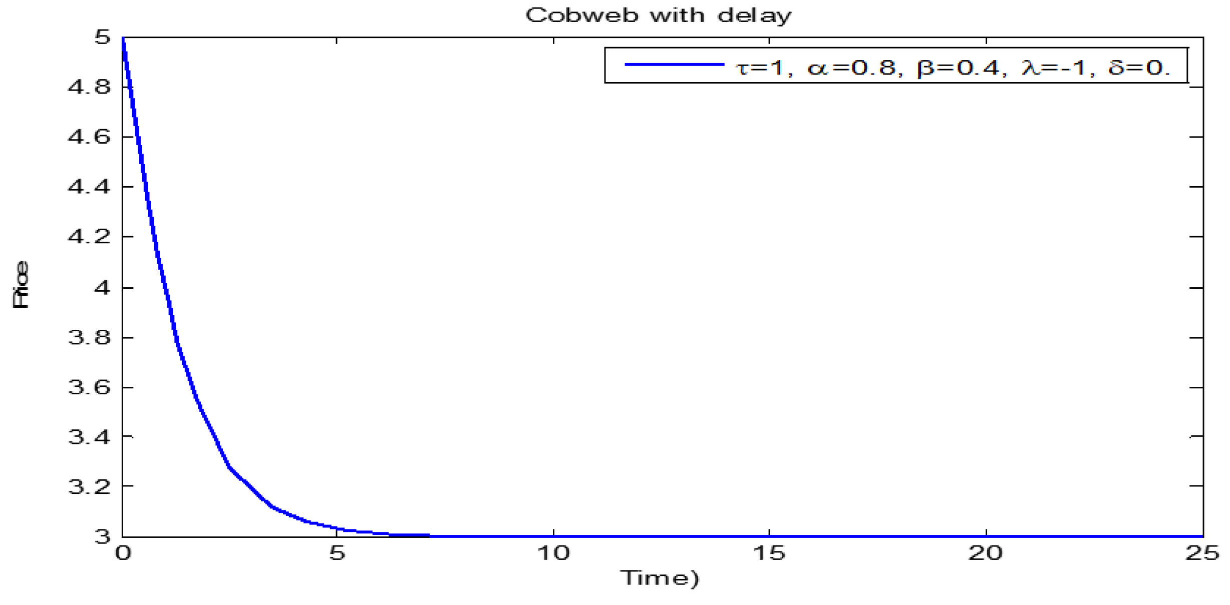
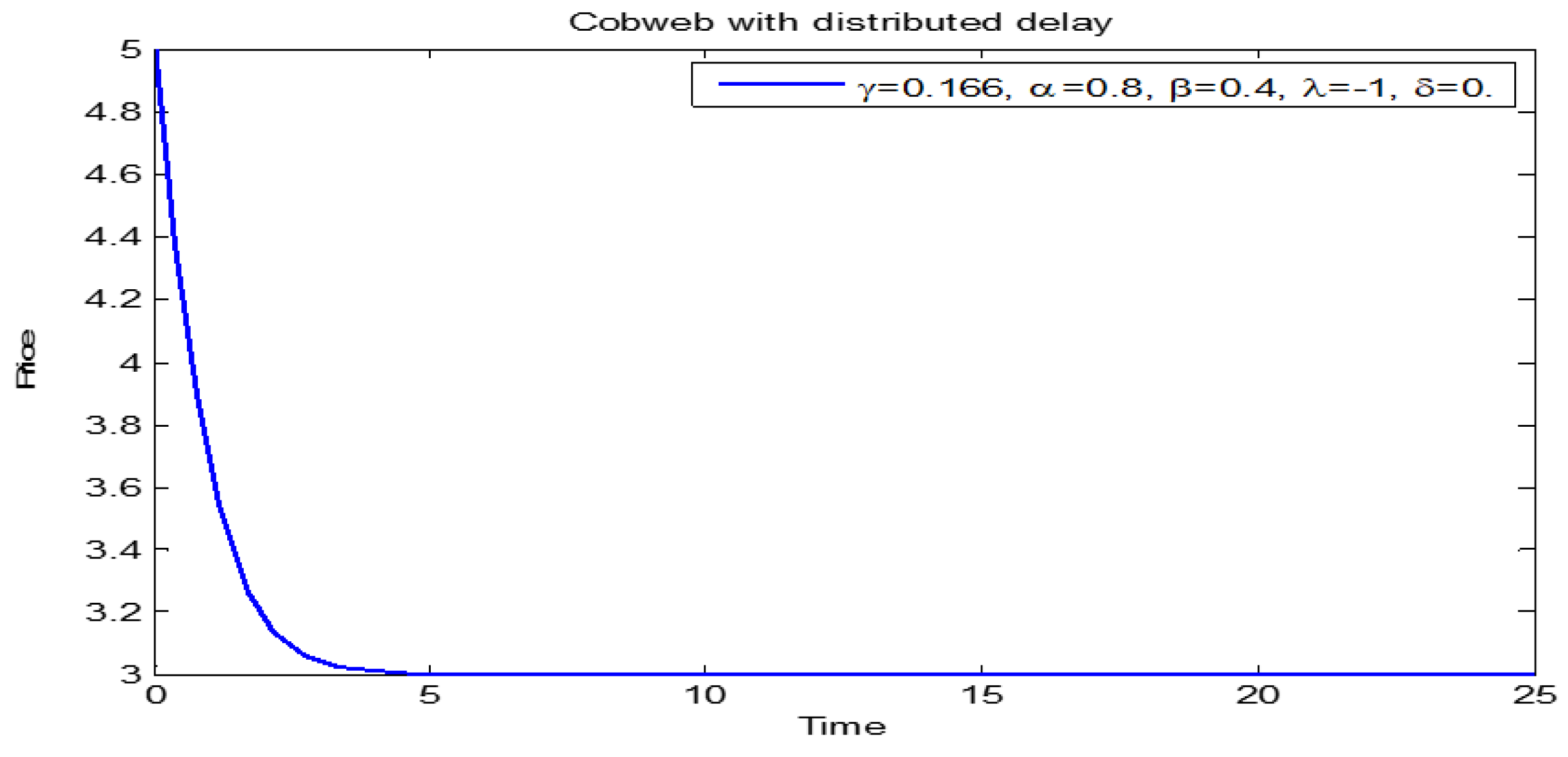
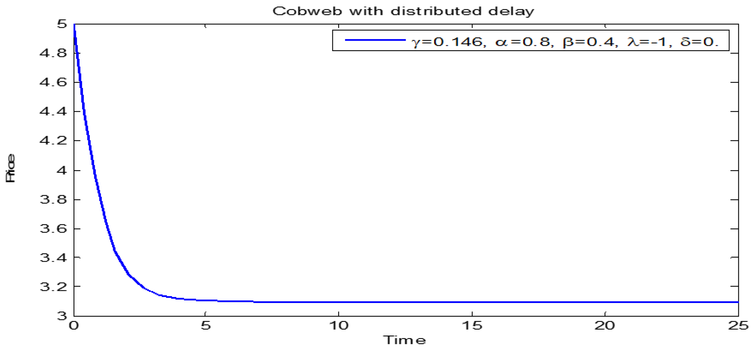
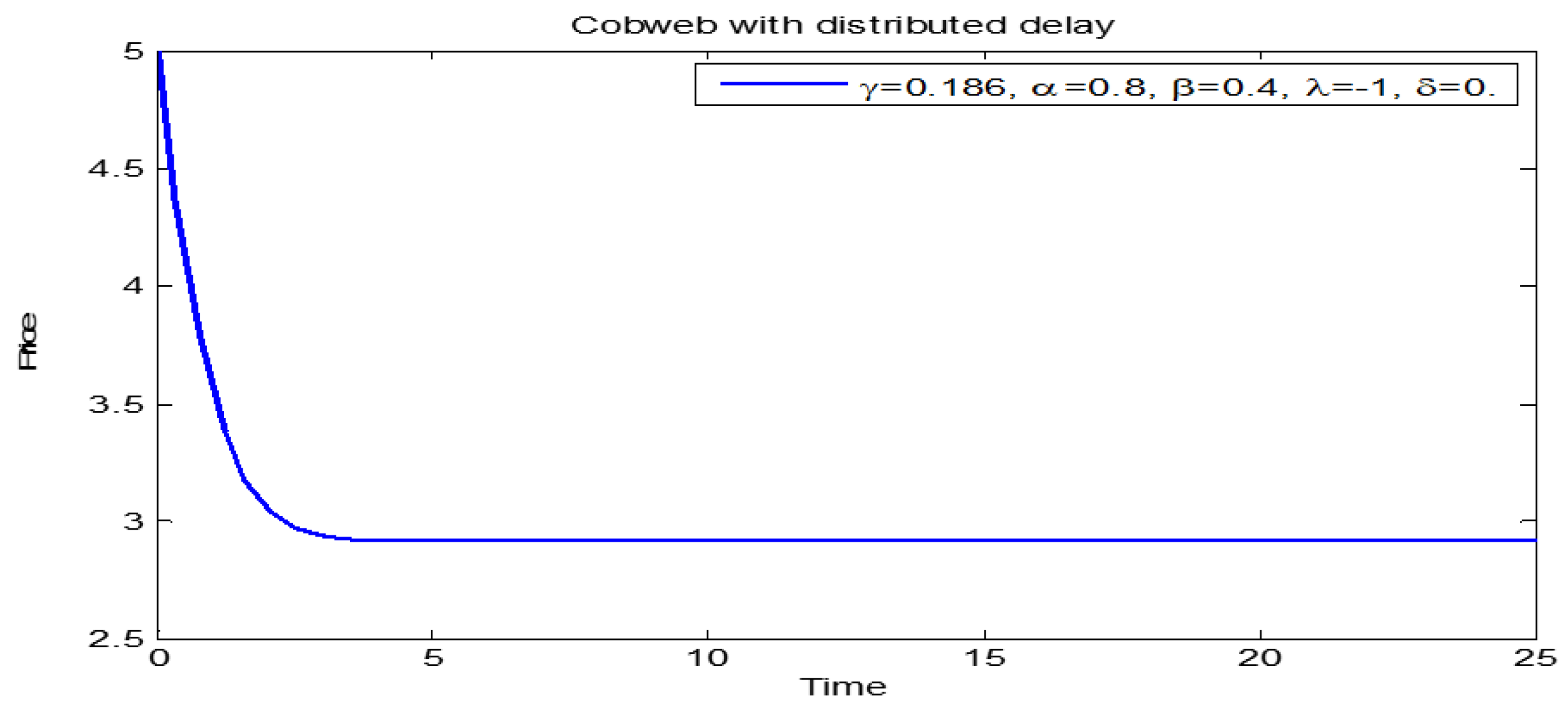
3.1. Price Dynamics of Models (1) and (2)

In this section, we adopt the same parameter values used in [18] and compare the stability analysis of our model (2) with the stability analysis of the existing model (1). Specifically, we utilize the following parameters: $\alpha =0.8$, $\beta =0.4$, $\lambda =1$ and $\delta =0.2$, from which we derive an equilibrium price of $p_e=3.0$, with an initial price of $p_0=5.0$. All numerical simulations are conducted using MATLAB software (MATLAB 2009b).

From Figure 1, it is observed that at a time delay of $\tau =1.0$ model (1) displayed similar dynamics, as shown in the previous work by Anokye et al. [18]. The price converged from an initial price of $p_0=5$ to the equilibrium price at $p_e=3$.

In Figure 2, where a generalized model, i.e., the distributed delay model (2), was considered with time delay at $\tau =1.0$ among several delays in the span of $[1,11]$, the model (2) exhibited similar dynamics in [18] when the kernel was set at $\gamma =0.166$. The delay kernel represents the weight the model assigns to the previous price in determining the current price. Notably, this “weight” refers to the emphasis suppliers place on the past market price. While lower weight is typically associated with unfavorable prices, higher weight corresponds to favorable prices.

In Figure 3, it is shown that when the weight is set at $\gamma =0.146$ (i.e., a decrease of 0.02), the equilibrium price is increased to $p_e=3.1$ from $p_e=3.0$ (compared to Figure 1). This demonstrates that the less weight assigned to the past price, the higher the current market price becomes. Practically, this suggests that when less emphasis is placed on the previous market price, it results in a lower supply of the product, thereby driving up the present market price (as indicated by $\gamma =0.146$) above the equilibrium price of $p_e=3.0$.

In Figure 4, it is shown that when the weight is increased to $\gamma =0.186$ (i.e., an increase of 0.02), the equilibrium price decreases from $p_e=3.0$ to $p_e=2.90$. This demonstrates that the higher the weight assigned to the past price, the lower the current market price becomes. In practical terms, this suggests that more emphasis was placed on the previous market price (i.e., the delay kernel effect), leading to an oversupply of commodities in the market, which in turn reduced the equilibrium price. These price dynamics are not present in the existing model (1), making our model (2) particularly intriguing and insightful.

3.2. Dynamics of Initial Price below the Equilibrium Price

In this section, we set the expected price above the initial market price to evaluate how the delay kernel should be adjusted to align the price dynamics of model (2) with those of the existing model (1). Let the expected price be $p_e=3.0$, with the initial price set as $p_0=1.0$, and time delay parameter $\tau =2.5$ while keeping all other parameter values the same as the previous subsection. This setup allows us to examine how adjustments in the delay kernel can bring the behavior of model (2) into conformity with the dynamics of model (1) when the initial market price starts below the expected price.

In Figure 5, when the time delay is increased to $\tau =2.5$ and the initial price is below the equilibrium price, we can see that the price behavior from model (1) initially moves above the equilibrium price at the onset of equilibrium (i.e., turning point) before finally converging to the equilibrium price of $p_e=3$ from the initial price of $p_0=1$. This sharp movement is a result of the higher time delay incorporated in the supply function of price in the model.

When the initial price is set below the equilibrium price, as observed in Figure 6, model (2) with a time delay at $\tau =2.5$ consistently leads to a decrease in weight from $\gamma =0.166$ (compared to Figure 2) to $\gamma =0.146$, causing the equilibrium price to move to $p_e=3.1$ from $p_e=3.0$ with an initial price of $p_0=1.0$. This situation typically favors the suppliers as less weight is associated with unfavorable past prices from the previous market.

When the equilibrium price is set above the initial price, as demonstrated in Figure 5, Figure 6 and Figure 7 with the same time delay of $\tau =2.5$, there was a decrease in the equilibrium price from $p_e=3.0$ to $p_e=2.90$ through convergence from an initial price of $p_0=1.0$, while the weight increased from $\gamma =0.166$ to $\gamma =0.186$. This situation, on the contrary, favors the consumers, as high weight is associated with a favorable price from the past market, motivating suppliers to increase yield to exceed demand at the market.

3.3. Dynamics of Initial Price below the Equilibrium Price

This section also addresses the scenario where the elasticity rule is subjected to an economic test. It is established that for convergence to occur, the price supply elasticity $\delta$ should be less than the demand elasticity $\beta$; otherwise, no price equilibrium will be achieved. We set $\beta =0.2$, $\delta =0.8$, and $\tau =2.5$, while keeping the other parameters constant as used in the previous subsection.

In Figure 8, it is demonstrated that with a time delay of $\tau =2.5$, when the price elasticity of supply $\delta =0.8$ is greater than the price elasticity of demand $\beta =0.2$, the price will infinitely oscillate around the equilibrium price, meeting the condition for divergence of the Cobweb model.

Figure 9 shows that for model (2) with the same parameter values as in Figure 8, and a delay kernel at $\gamma =0.166$, the price exhibits a few oscillations and converges to equilibrium, even though the elasticity of supply $\delta =0.8$ is greater than the price elasticity of demand $\beta =0.2$. This dynamic defies the condition for divergence of the cobweb model, as it depends on the weight placed on the past price rather than how the elasticity of supply relates to that of the demand elasticity. The reality is that the weight (i.e., delay kernel) predicts the occurrence of the price scenarios for stakeholders to take the necessary steps to keep the commodity price stable.

Note that the delay kernel parameter $\gamma =0.166$ is utilized to guarantee that the prices of both the fixed delay cobweb model (1) and the distributed delay model (2) will converge to the same market equilibrium price. However, model (1) did not achieve this. Values lower than $\gamma =0.166$ lead to further price increases, while values greater than $\gamma =0.166$ result in price decreases. This encapsulates the dynamics of the system.

4. Conclusions

This paper explores the stability and occurrence of Hopf bifurcation in a delay-distributed differential cobweb model using the chain trick technique. This model is a generalized form of the fixed delay cobweb model, and the two are compared using identical parameter values. The results indicate that when a lower weight $(\gamma =0.146)$ is assigned to past prices, the current equilibrium price adjusts upwards, while a higher weight $(\gamma =0.186)$ leads to a downward adjustment. Additionally, if the initial price is set either below or above the equilibrium price, the resulting price adjustments can either negatively impact consumers or benefit suppliers. Interestingly, the fixed delay cobweb model does not exhibit these consumer or supplier effects in its price dynamics. These unique patterns in price behavior observed in the distributed delay model set it apart from traditional fixed delay models. Moreover, this model challenges the conventional cobweb theory’s requirement for divergence, as it is influenced by the weight placed on past prices rather than the elasticity relationship between supply and demand, as seen in existing models. From a managerial perspective, commodity suppliers, by considering the impact of past prices (i.e., the weight on previous prices), may make decisions that could affect the market either positively or negatively. However, a key limitation of this study is that model (2) operates under the assumption that only past prices (naive price expectations) are used for decision-making, with all other factors held constant. Other types of price expectations, such as rational price expectations, were not considered but could be explored in future research. Consequently, it is recommended that future price adjustment models incorporate distributed delays to capture these more nuanced dynamics.

References

1. Chen, C.; Bohner, M.; Baoguo, J. Caputo fractional continuous cobweb models. J. Comput. Appl. Math. 2020, 374, 112734. [Google Scholar] [CrossRef]
2. Brianzoni, S.; Mammana, C.; Michetti, E.; Zirilli, F. A stochastic cobweb dynamical model. Discrete Dyn. Nat. Soc. 2008, 18, 219653. [Google Scholar] [CrossRef]
3. Nerlove, M. Adaptive expectations and cobweb phenomena. Q. J. Econ. 1958, 72, 227–240. [Google Scholar] [CrossRef]
4. Muth, J.F. Rational expectations and the theory of price movements. Econometrica 1961, 29, 315–335. [Google Scholar] [CrossRef]
5. Hommes, C.H. Adaptive learning and roads to chaos: The case of the cobweb. Econom. Lett. 1991, 36, 127–132. [Google Scholar] [CrossRef]
6. Hommes, C.H. Cobwebs, chaos and bifurcations. Ann. Oper. Res. 1992, 37, 97–100. [Google Scholar] [CrossRef]
7. Gaffney, J.M.; Pearce, C.E.M. Nonlinear-cobweb dynamics in the approach to equilibrium. ANZIAM J. 2004, 46, 79–83. [Google Scholar] [CrossRef]
8. Ezekiel, M. The cobweb Theorem. Q. J. Econ. 1938, 52, 255–280. [Google Scholar] [CrossRef]
9. Nagy, A.M.; Assidi, S.; Ben Makhlouf, A. Convergence of solutions for perturbed and unperturbed cobweb models with generalized Caputo derivative. Bound. Value Probl. 2022, 2022, 89. [Google Scholar] [CrossRef]
10. Dufresne, D.; Vazquez-Abad, F. Cobweb theorems with production lags and price forecasting. Economics-Kiel 2013, 7, 20130023. [Google Scholar] [CrossRef]
11. Eltayeb, H.; Abdeldaim, E. Sumudu decomposition method for solving fractiona delay differential equations. Res. Appl. Math. 2017, 1, 101268. [Google Scholar] [CrossRef]
12. Ma, J.; Lingling, M. Complex dynamics in a nonlinear cobweb model for real estate market. Discrete Dyn. Nat. Soc. 2007, 2007, 29207. [Google Scholar] [CrossRef]
13. Matsumoto, A.; Szidarovszky, F. The asymptotic behavior in a nonlinear cobweb model with time delays. Discrete Dyn. Nat. Soc. 2015, 2015, 12574. [Google Scholar] [CrossRef]
14. Gori, L.; Guerrini, L.; Sodini, M. Hopf bifurcation and stability crossing curves in a cobweb model with heterogeneous producers and time delays. Nonlinear Anal. Hybrid Syst. 2015, 18, 117–133. [Google Scholar] [CrossRef]
15. Gori, L.; Guerrini, L.; Sodini, M. Equilibrium and disequilibrium dynamics in cobweb models with time delays. Int. J. Bifurc. Chaos 2015, 25, 1550088. [Google Scholar] [CrossRef]
16. Gori, L.; Guerrini, L.; Sodini, M. Hopf bifurcation in a cobweb model with discrete time delays. Discrete Dyn. Nat. Soc. 2014, 37090. [Google Scholar] [CrossRef]
17. Matsumoto, A.; Nakayama, K. Nonlinear cobweb model with time delays. Int. Conf. Model. Simul. Appl. Math. 2015, 402–406. [Google Scholar]
18. Anokye, M.; Barnes, B.; Boateng, F.O.; Adom-Konadu, A.; Amoah-Mensah, J. Price dynamics of a delay differential Cobweb model. Discrete Dyn. Nat. Soc. 2023, 2023, 296562. [Google Scholar] [CrossRef]
19. Miller, R.K. Asymptotic stability properties of linear Volterra integro-differential equations. J. Differ. Equ. 1971, 10, 485–506. [Google Scholar] [CrossRef]
20. Kar, M. Pricing strategies in mobile telecommunications markets. Smart J. 2019, 5, 360–371. [Google Scholar] [CrossRef]
21. Doldo, P.; Pender, J. A note on the interpretation of distributed delay equations. arXiv 2021, arXiv:2106.11413. [Google Scholar]
22. Elaiw, A.M.; Al Agha, A.D. A reaction-diffusion model for oncolytic M1 virotherapy with distributed delays. Eur. Phys. J. Plus 2020, 135, 117. [Google Scholar] [CrossRef]
23. Elowitz, M.B.; Levine, A.J.; Siggia, E.D.; Swain, P.S. Stochastic gene expression in a single cell. Science 2002, 297, 1183–1186. [Google Scholar] [CrossRef] [PubMed]
24. Arjun, R.; Van Oudenaarden, A. Nature, nurture, or chance: Stochastic gene expression and its consequences. Cell 2008, 135, 216–226. [Google Scholar]
25. McAdams, H.H.; Arkin, A. Stochastic mechanisms in gene expression. Proc. Natl. Acad. Sci. USA 1996, 94, 814–819. [Google Scholar] [CrossRef]
26. Paulsson, J. Models of stochastic gene expression. Phys. Life Rev. 2005, 2, 157–175. [Google Scholar] [CrossRef]
27. Sargood, A.; Gaffney, E.A.; Krause, A.L. Fixed and distributed gene expression time delays in reaction-diffusion systems. Bull. Math. Biol. 2022, 84, 98. [Google Scholar] [CrossRef]
Figure 1. Price dynamics of cobweb model (1) with  τ = 1 .
Mathematics 12 03220 g001
Figure 2. Price dynamics of cobweb model (2) with delay kernel  γ = 0.166 .
Mathematics 12 03220 g002
Figure 3. Price dynamics of cobweb model (2) with delay kernel  γ = 0.146 .
Mathematics 12 03220 g003
Figure 4. Price dynamics of cobweb model (2) with delay kernel  γ = 0.186 .
Mathematics 12 03220 g004
Figure 5. Price dynamics of cobweb model (1) with  τ = 2.5 .
Mathematics 12 03220 g005
Figure 6. Price dynamics of cobweb model (2) with p0 < pe and delay kernel  γ = 0.146 .
Mathematics 12 03220 g006
Figure 7. Price dynamics of cobweb model (2) with p0 < pe and delay kernel  γ = 0.186 .
Mathematics 12 03220 g007
Figure 8. Price dynamics of cobweb model (1) with elasticity  β < δ .
Mathematics 12 03220 g008
Figure 9. Price dynamics of cobweb model (2) with elasticity  β < δ .
Mathematics 12 03220 g009
Disclaimer/Publisher’s Note: The statements, opinions and data contained in all publications are solely those of the individual author(s) and contributor(s) and not of MDPI and/or the editor(s). MDPI and/or the editor(s) disclaim responsibility for any injury to people or property resulting from any ideas, methods, instructions or products referred to in the content.