SVSeq2Seq: An Efficient Computational Method for State Vectors in Sequence-to-Sequence Architecture Forecasting

Abstract

This study proposes an efficient method for computing State Vectors in Sequence-to-Sequence (SVSeq2Seq) architecture to improve the performance of sequence data forecasting, which associates each element with other elements instead of relying only on nearby elements. First, the dependency between two elements is adaptively captured by calculating the relative importance between hidden layers. Second, tensor train decomposition is used to address the issue of dimensionality catastrophe. Third, we further select seven instantiated baseline models for data prediction and compare them with our proposed model on six real-world datasets. The results show that the Mean Square Error (MSE) and Mean Absolute Error (MAE) of our SVSeq2Seq model exhibit significant advantages over the other seven baseline models in predicting the three datasets, i.e., weather, electricity, and PEMS, with MSE/MAE values as low as 0.259/0.260, 0.186/0.285 and 0.113/0.222, respectively. Furthermore, the ablation study demonstrates that the SVSeq2Seq model possesses distinct advantages in sequential forecasting tasks. It is observed that replacing SVSeq2Seq with LPRcode and NMTcode resulted in an increase under an MSE of 18.05 and 10.11 times, and an increase under an MAE of 16.54 and 9.8 times, respectively. In comparative experiments with support vector machines (SVM) and random forest (RF), the performance of the SVSeq2Seq model is improved by 56.88 times in the weather dataset and 73.78 times in the electricity dataset under the MSE metric, respectively. The above experimental results demonstrate both the exceptional rationality and versatility of the SVSeq2Seq model for data forecasting.

1. Introduction

Sequential data forecasting is a fundamental inquiry in science: to what extent can we anticipate the future from historical data? Forecasting future data states from past data states is an intriguing and arduous task in numerous fields, such as energy and smart grid management, sensor network monitoring, and disease propagation analysis [1].

At present, several forecasting techniques have been developed for sequential data forecasting, such as Recurrent Neural Network (RNN)-based methods [2,3], Transformer-based methods [4,5], Linear-based methods [6,7], and TCN-based methods [8,9], which have achieved immense success in extensive fields. Transformer-based methods such as Informer [10], Autoformer [4], and Crossformer [5] have great advantages in managing remote and complex dependencies. Nevertheless, they often require substantial computational resources and memory, which increases the risk of overfitting large Transformer models with limited data. Linear-based methods such as DLinear [6] and TiDE [7] exhibit high computational efficiency and strong interpretability; however, the dependency on linear transformation makes them more suitable for dealing with simple sequence tasks, but the feature extraction ability is weak. TCN-based methods such as SCINet [8] and TimesNet [9] have obvious advantages in terms of computational efficiency and number of parameters, but they tend to prioritize the capture of local features and may fall short in identifying long-term dependencies.

Notably, in comparison to the above methods, RNN-based methods such as Long Short-Term Memory (LSTM) [2] and Gated Recurrent Unit (GRU) [3] inherently model sequential data with remarkable parameter efficiency and exhibit superior capabilities in handling extended sequences. RNN-based methods have attracted increasing attention in the field of sequential data forecasting due to their superior capabilities in handling extended sequences. For example, in 2014, Cho et al. [3] proposed the RNN encoder–decoder model using the hidden states as state vectors, which utilized one RNN to encode a sequence of symbols as a fixed-length vector representation, and another RNN to decode the representation as another sequence of symbols. In 2022, Li et al. [11] introduced the Multi-Dimensional Spatial-Temporal Recurrent Neural Network (MST-RNN), an approach that leveraged both the temporal duration and semantic tag dimensions of Points of Interest (POIs) in each layer of the neural network framework. In 2023, Jadhav et al. [12] introduced two methods for analyzing dynamic relationships within real-world sequential data: the Internal Time-Varying sequence model (ITV model) and the External Time-Varying sequence model (ETV model). Their models were distinguished by an automated basis expansion module that dynamically adapted internal or external parameters with each time step, thereby minimizing computational complexity. In addition, RNN-based methods often use a Sequence-to-Sequence structure to handle dialogue, translation, and prediction tasks [2]. In 2014, Google [13] proposed the Sequence-to-Sequence structure as a common structure for RNN-based methods, which can be simply understood as consisting of three parts: the encoder, the decoder, and the state vector connecting them. The encoder comprehended the input sequence to produce the state vector, and the decoder utilized the state vector as an input to eventually generate an output that satisfied the given task requirements [2,3].

As one of the important components of RNN based on Sequence-to-Sequence structure, improving the computation method of the state vector is crucial to enhance the performance of complex forecasting, as it is the only channel connecting the encoder output to the decoder input and thus has a significant impact on the final output result [14]. At present, many elaborate designs of state vectors for RNN-based improvement models have been proposed to solve the ubiquitous applications of serial forecasting. For example, Serban et al. [15] and Sordoni et al. [16] both used a context RNN for efficient sequence data prediction. Notably, these methods still struggle to capture global patterns and exacerbate the negative impact of noisy data on long-term dependencies, resulting in inadequate long-term forecasting. Furthermore, to improve the shortcomings of the above models, Serban et al. proposed the Latent Variable Hierarchical Recurrent Encoder–Decoder (VHRED) model [17], which incorporated a latent variable into the decoder and was trained by maximizing the log-likelihood. In addition, Weston et al. [18] introduced a class of memory networks that combined successful learning strategies with a memory component. Further, Fernando et al. [19] proposed a tree memory network to jointly model long-term relationships, where the method employed the output of the input module as a state vector. The above methods lack personalized state vectors for the different hidden layers of the decoder; consequently, they often strive to achieve superior performance in complex prediction tasks. To further improve the performance of data forecasting, Sennrich et al. [14] calculated the state vector by computing weight vectors and summing the hidden states of the encoder. Although this method considered all the input vectors, it did not consider the positional information of the vectors. In 2023, Cao et al. [20] introduced an end-to-end encoder–decoder structure, which introduced the meta-path augmented residual information matrix to preserve the structure evolution mechanism and semantics in HINs, and used it as input to the encoder to obtain a low-dimensional embedding representation of the nodes.

Consequently, improving the state vector calculation method will enable RNN-based methods to achieve commendable predictive performance in sequence forecasting. Google [13] first introduced the Transformer, an approach that relied solely on the attention mechanism, garnering significant achievements in areas such as natural language processing [21] and computer vision [22]. Currently, many elaborate Transformer variants have been proposed, such as Autoformer [4], non-stationary Transformers [23], and the PatchTST model [24], to address ubiquitous serial forecasting applications. These attention mechanism-based methods fully leverage the positional information of all vectors. Attention mechanism has not only shown good performance in sequence data prediction but has also been used to automatically synthesize high-quality images from textual descriptions. For example, Chopra et al. [25] proposed the AttnGAN method, which used an attentional model to generate sub-regions of an image based on the description. Inspired by the immense success of the attention mechanism in extensive fields, the attention mechanism used to compute the state vector in the Sequence-to-Sequence structure will effectively improve the prediction performance.

In this paper, we propose an innovative and efficient method for computing State Vectors in Sequence-to-Sequence (SVSeq2Seq) architecture. In this strategy, the attention mechanism is meticulously designed as the computational method of state vectors for Sequence-to-Sequence structure, which has enhanced capabilities in sequence modeling. Consequently, the proposed SVSeq2Seq effectively exploits the relationship between the hidden layers of the decoder and those of the encoder, thereby demonstrating superior capabilities in predicting sequential data. SVSeq2Seq comprises state vector weighting and tensor train networks. Our contribution can be summarized as follows:

(i) We use the relative significance between hidden layers to dynamically capture the interdependent aspects among elements. We then compute weight vectors for the encoder’s hidden layers based on these dependencies. We then provide adaptive state vector weights based on the computed weight vectors.

(ii) We apply tensor train decomposition to fit the expansion tensor, which successfully counteracts the problem of high dimensionality.

(iii) We confirmed the outstanding performance of SVSeq2Seq on six authentic datasets, showing significant advantages over the other seven baseline models in predicting the three datasets. We also performed ablation experiments on three of these datasets, confirming the rationality and generalizability of SVSeq2Seq. Finally, we compare the prediction effect before and after deleting all state vector components in the experimental process, which proves the importance of SVSeq2Seq in the Sequence-to-Sequence structure.

2. Model Descriptions and Preliminaries

In this study, we introduce an efficient computational method for state vectors in Sequence-to-Sequence structure forecasting, i.e., SVSeq2Seq, which incorporates state vector weights and tensor train networks. As shown in Figure 1, SVSeq2Seq records the hidden layers of the encoder (red line) and computes their correlation with the hidden layers of each decoder (green line), thus providing personalized state vectors for the hidden layers of each decoder.

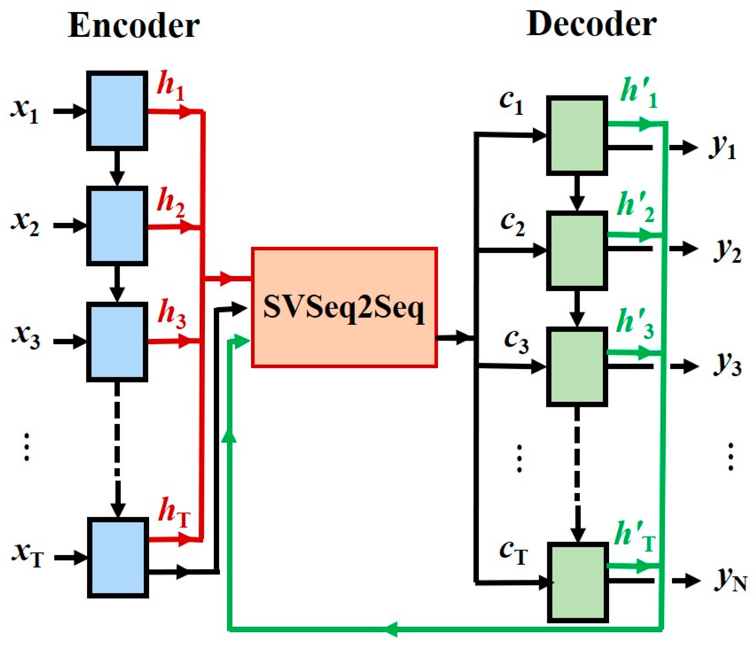
2.1. Encoder–Decoder Architecture of the RNN

First, the fundamental framework of the encoder–decoder architecture of the RNN is outlined, and based on this, an efficient strategy for state vector computation is developed.

In the encoder–decoder architecture, the encoder processes the input vector $\mathrm{x}=\left\{x_1,\dots ,x_{\mathrm{T}}\right\}$ and transforms it into a state vector $c$. The most common approach is to use an RNN, as shown in Equations (1) and (2):

$$h_t=f(x_t,h_{t-1})$$

(1)

and

$$c=q\left(\{h_1,\cdots ,h_{\mathrm{T}}\}\right),$$

(2)

where $h_t\in {\mathbb{R}}^n$ is a hidden state at time $t$, and $c$ is a vector generated from the sequence of the hidden states. The function $f$ can be a non-linear equation, with examples being naïve RNN, LSTM, or GRU, and $q\left(\right\{h_1,\cdots ,h_{\mathrm{T}}\left\}\right)=h_{\mathrm{T}}.$

The decoder derives the output $y_{t^{\prime }}$ utilizing the state vector $c$. In the context of the translation tasks, it is common for the decoder to establish a probability for the translation $y$, which is achieved by decomposing the joint probability into ordered conditionals, as shown in Equation (3):

$$p\left(y\right)={\prod }_{t=1}^{\mathrm{T}}\hspace{0.17em}p(y_t\mid \left\{y_1,\cdots ,y_{t-1}\right\},c),$$

(3)

where $y=\left(\begin{array}{c}{y}_1,\cdots ,y_{{\mathrm{T}}_y}\end{array}\right).$ Using an RNN, each conditional probability is formulated, as shown in Equation (4):

$$p(y_t\mid \{y_1,\cdots ,y_{t-1}\},c)=g(y_{t-1},h_t,c),$$

(4)

where $g$ is a non-linear function that outputs the probability of $y$ while $h$ is the hidden state of the RNN.

Within the Sequence-to-Sequence framework, the decoder has the capability to generate multiple $y_{t^{\prime }}$ by interpreting the state vector $c$.

As described above, the encoder produces the state vector $c$, which the decoder then uses to output the desired result $y$. Given the significant influence of the state vector $c$ on the output within the encoder–decoder framework, we propose an efficient approach to compute the state vector in the Sequence-to-Sequence structure.

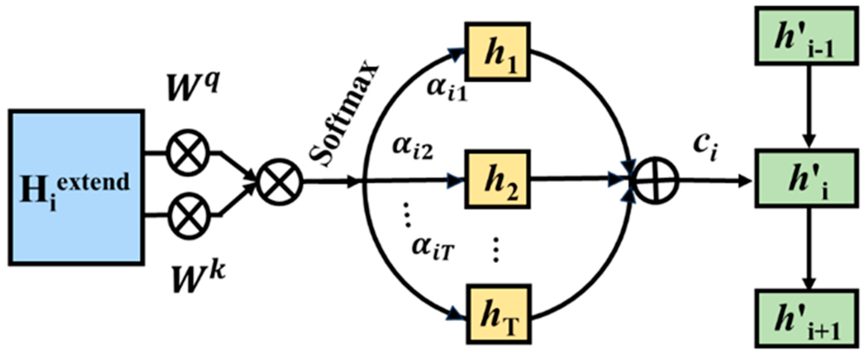
2.2. State Vector Computation

In our efficient state vector computation approach, we leverage the correlation between the decoder’s hidden layer $h^{\prime }$ and the encoder’s hidden layer $h$ to compute the weight $a$ of distinct $h$. This method allows us to generate unique state vectors $c$ corresponding to different $h^{\prime }$. Figure 2 illustrates the entire process of computing the state vector $c$.

The state vector $c$ depends on a sequence of $\{{h_1^{\prime },h}_1,\cdots ,h_{\mathrm{T}}\}$ onto which an encoder maps the input $\left\{x_1,\dots ,x_{\mathrm{T}}\right\}$. Each $h_i$ contains information about the whole input with a strong focus on the parts surrounding the i-th input. The state vector $c$ is computed by a weighted sum of $\{{h_1^{\prime },h}_1,\cdots ,h_{\mathrm{T}}\}$, as shown in Equation (5):

$$c_i={\sum }_{j=1}^{\mathrm{T}}\hspace{0.17em}{\alpha }_{ij}{h}_j.$$

(5)

We assume that the decoder input is $x_1^{\prime },x_2^{\prime },\dots ,x_{t^{\prime }}^{\prime }$. Since $x_1^{\prime }$ and $h_1^{\prime }$ are known, we can calculate $y_1$. This allows us to set $x_2^{\prime }=y_1$, indicating that the output from one time step becomes the input for the next. One might wonder about the origin of $x_1^{\prime }$. Typically, we use the special character “<BOS>” (beginning of sentence) to denote the beginning of an input $x_1^{\prime }$. The terminating condition reflects this approach. Specifically, the forecasting process terminates when the output is a special character “<EOS>” (end of sentence).

Let us use $h_1^{\prime }$ as a case study to illustrate the computation of the weight ${\alpha }_{1j}$. To start off, we establish two weight matrices, denoted as $W^q$ and $W^k$, as shown in Equation (6):

$$\left\{\begin{array}{c}{q}^1=w_1^q·h_1^{extend}\\ k^1=w_1^k·h_1^{extend}\end{array}{h}_1^{extend}=\{{h_1^{\prime },h}_1,\cdots ,h_{\mathrm{T}}\}\right.$$

(6)

Let us express this in vector form in Equation (7):

$$\left\{\begin{array}{c}Q=W^q·H_i^{extend}\\ K=W^k·H_i^{extend}\end{array}{H}_i^{extend}=\{{h_i^{\prime },h}_1,\cdots ,h_{\mathrm{T}}\}\right.$$

(7)

We use $Q$ and $K$ to compute the correlation between $h_i^{\prime }$ and the elements within the set $\{h_1,\cdots ,h_{\mathrm{T}}\}$ in $H_i^{extend}$, denoted as $a_{ij}^{\prime }$ and computed as Equation (8):

$$a_{ij}^{\prime }=(q^i{)}^{\tau }\cdot k^j$$

(8)

Let us express this in vector form in Equation (9):

$$A^{\prime }=K^{\mathrm{T}}·Q$$

(9)

The softmax operation is applied to the $A^{\prime }$ matrix, ensuring that its elements fall within the range [0, 1], and the result is denoted as $A$ in Equation (10):

$$A=softmax\left(A^{\prime }\right)$$

(10)

The state vector $c$ is computed by substituting the elements ${\alpha }_{ij}$ of the matrix $A$ into Equation (5).

To illustrate the computation process of the state vectors $c$, Algorithm 1 is provided, which shows the pseudocode in detail.

Algorithm 1: State vectors $c$

Input: The input vector $\left\{x_1,\dots ,x_{\mathrm{T}}\right\}$ of Encoder and $H_i^{extend}$  Output: State vectors $c$ 1 for $x_i$ in $\left\{x_1,\dots ,x_{\mathrm{T}}\right\}$ do 2  Calculate $q^i$ and $k^j$, Equation (7); 3  Calculate $a_{ij}^{\prime }$, Equation (8); 4  Express $a_{ij}^{\prime }$ in vector form, Equation (9); 5  Make sure the elements in $A^{\prime }$ within [0, 1], Equation (10); 6  Take the elements ${\alpha }_{ij}$ of $A$ into Equation (5); 7 ends 8 Get $c_i={\sum }_{j=1}^{\mathrm{T}}\hspace{0.17em}{\alpha }_{ij}{h}_j$

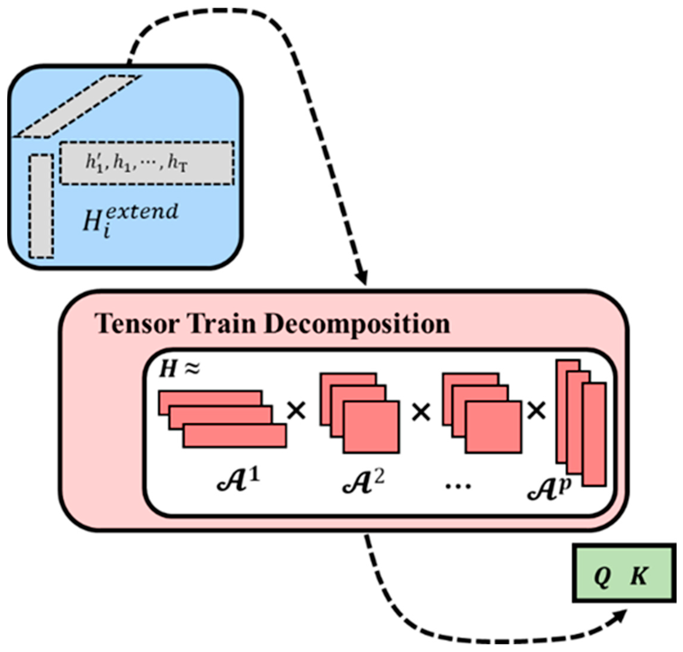
2.3. Tensor Train Networks

As the number of hidden layers in the encoder and decoder increases, the size of $H^{extend}$ also expands rapidly. This expansion complicates the computation of Equations (7) and (9), and consequently requires a larger size for training. To overcome this difficulty, we use tensor networks to approximate $H^{extend}$. Such networks encode a structural decomposition of tensors into low-dimensional components and have been shown to provide the most general approximation to smooth tensors (Figure 3) [26].

A tensor train model decomposes a $P$-dimensional tensor $H^{extend}$ into a network of sparsely connected low-dimensional tensors $\{{\mathcal{A}}^p\in {\mathbb{R}}^{r_{p-1}\times n_p\times r_p}\}$ such that Equation (11)

$$H_{i_1\cdots i_P}={\sum }_{{\alpha }_1\cdots {\alpha }_{P-1}}\hspace{0.17em}{\mathcal{A}}_{{\alpha }_0{i}_1{\alpha }_1}^1{\mathcal{A}}_{{\alpha }_1{i}_2{\alpha }_2}^2\cdots {\mathcal{A}}_{{\alpha }_{P-1}{i}_P{\alpha }_P}^P$$

(11)

In Equation (11), ${\alpha }_0={\alpha }_P=1.$ When $r_0=r_P=1$, the $\left\{r_p\right\}$ is called the rank of the tensor train. With tensor trains, we can reduce the number of parameters from ${(q+k)}^{\mathrm{T}+1}$ to $(q+k)R^2(\mathrm{T}+1)$, with $\mathrm{R}={max}_p{r}_p$ as the upper bound of the tensor train rank. Thus, a major advantage of tensor trains is that they do not suffer from the curse of dimensionality, which is in sharp contrast to many classical tensor decomposition models, such as the Tucker decomposition.

3. Experiment Results

3.1. Experimental Setup

To verify the effectiveness of our state vector computation method, we constructed a Sequence-to-Sequence structure using an LSTM. For all experiments, we used an initial sequence of length $t_0$ as input and varied the prediction time horizon T. We trained all models using stochastic gradient descent, with a regression loss function $L(y,\widehat{y})={\sum }_{t=1}^{\mathrm{T}}\hspace{0.17em}\left|\right|{\widehat{y}}_t-y_t|{|}_2^2$ applied to sequences of length T. In this case, $y_t=x_{t+1}$ represents the true values, while ${\widehat{y}}_t$ represents the predicted values from our model.

Two conventional machine learning-based methods, such as Support Vector Machines (SVM) and Random Forest (RF), were selected as the baselines to compare the performance with our proposed model. Further, we also selected seven popular prediction models as benchmarks from three categories, including Transformer-based methods such as Informer [10], FEDformer [27], and Crossformer [5]; Linear-based methods such as DLinear [6] and TiDE [7]; TCN-based methods such as SCINet [8] and TimesNet [9].

3.2. Dataset Preparation

Six real-world datasets including Electricity Transformer Temperature (ETT), weather, electricity, traffic used by Autoformer [4], solar-energy datasets proposed in LSTNet [28] and Performance Measurement System (PEMS) evaluated in SCINet [8] were selected in our experiments.

3.2.1. ETT Dataset

ETT dataset encompasses temperature recordings of electrical transformers over a period and typically includes corresponding information on electricity usage. Spanning data from several months to several years, the ETT dataset is recorded at regular intervals, such as every 15 min, every half hour, or hourly. The applicability of the ETT dataset is extensive, especially in areas where accurate short-term or long-term predictions of electrical demand are needed. This includes analyzing and forecasting supply and demand dynamics in the electricity market, predicting residential and industrial electricity consumption patterns in energy usage, and conducting short-term and long-term load forecasting for power systems.

3.2.2. Weather Dataset

The weather dataset comprehensively records meteorological indicators at 10 min intervals throughout the year 2020, encompassing 21 variables including air temperature and humidity. The dataset’s scope of application is exceptionally broad, ranging from analyzing and forecasting climate change trends to tracking environmental shifts, assessing pollution and ecosystem health, and utilizing historical and real-time data for predicting both short-term and long-term weather conditions.

3.2.3. Electricity Dataset

The electricity dataset encompasses hourly electricity consumption data for 321 customers spanning from the year 2012 to 2014. The utility of this data is remarkably broad, encompassing applications such as analyzing energy consumption patterns to drive efficiency improvements, forecasting short-term or long-term loads in power systems, predicting electricity prices in the energy market based on supply and demand conditions, and monitoring anomalous behaviors within the electrical grid.

3.2.4. Traffic Dataset

The traffic dataset is a compilation of data collected by the California Department of Transportation, characterizing road occupancy rates measured by various sensors located on highways in the San Francisco Bay Area. This dataset is applicable to a wide range of uses, such as forecasting traffic flow at specific times and locations, identifying bottleneck segments and periods of congestion, and supporting infrastructure planning and development through the analysis of traffic patterns.

3.2.5. Solar-Energy Dataset

Solar-Energy dataset chronicles the solar energy production in the year 2006, with samples collected every 10 min from 137 photovoltaic power stations in Alabama. This dataset has a similarly extensive range of applications, such as forecasting the energy output of solar power stations or photovoltaic systems, investigating the relationship between solar radiation and climate change, and assessing the impact of different geographical locations and seasons on the performance of photovoltaic systems.

3.2.6. PEMS Dataset

PEMS collects and stores real-time traffic data from across the entire highway system in California, including metrics such as traffic volumes, vehicle speeds, and lane occupancy rates. This information is primarily obtained through inductive loop detectors and other sensors deployed on the highways. The system aggregates data both temporally (e.g., every 5 min) and spatially (e.g., per detection point or region), thereby supporting traffic management, planning, and research initiatives. Spanning a wide network of California’s highways, the dataset provides several years of historical data, proving invaluable for transportation research, urban planning, traffic engineering, and environmental impact assessments.

3.3. MAE and MSE Calculation

For the purposes of this experiment within the context of sequence prediction tasks, we have selected two prevalent and extensively utilized evaluation metrics, i.e., MSE and MAE. The MSE represents the average of the squares of the differences between the predicted and actual values. The computational method for MSE is delineated in Equation (12):

$$\mathrm{M}\mathrm{S}\mathrm{E}=\frac{1}{m}{\sum }_{i=1}^m\hspace{0.17em}(y_{test}^{\left(i\right)}-{\widehat{y}}_{test}^{\left(i\right)}{)}^2$$

(12)

where $m$ denotes the number of samples, $y_{test}^{\left(i\right)}$ represents the actual values, and ${\widehat{y}}_{test}^{\left(i\right)}$ signifies the predicted values by the model. The squared term in MSE accentuates the impact of larger errors, rendering it particularly sensitive to outliers. This attribute can be advantageous in certain scenarios, such as when substantial prediction errors entail more severe consequences than minor ones. As a differentiable function, MSE possesses favorable mathematical properties during optimization processes, such as gradient descent, which are crucial for model training.

The MAE is the average of the absolute differences between the predicted values and the actual values. The MAE directly quantifies the average deviation between the predicted values and the actual values and is straightforward to interpret and comprehend. Due to the absence of a squared term, MAE is less sensitive to outliers compared to the MSE, offering a more robust error estimation in the presence of anomalous data points. The method for calculating MAE is presented in Equation (13):

$$\mathrm{M}\mathrm{A}\mathrm{E}=\frac{1}{m}{\sum }_{i=1}^m\hspace{0.17em}|y_{test}^{\left(i\right)}-{\widehat{y}}_{test}^{\left(i\right)}|$$

(13)

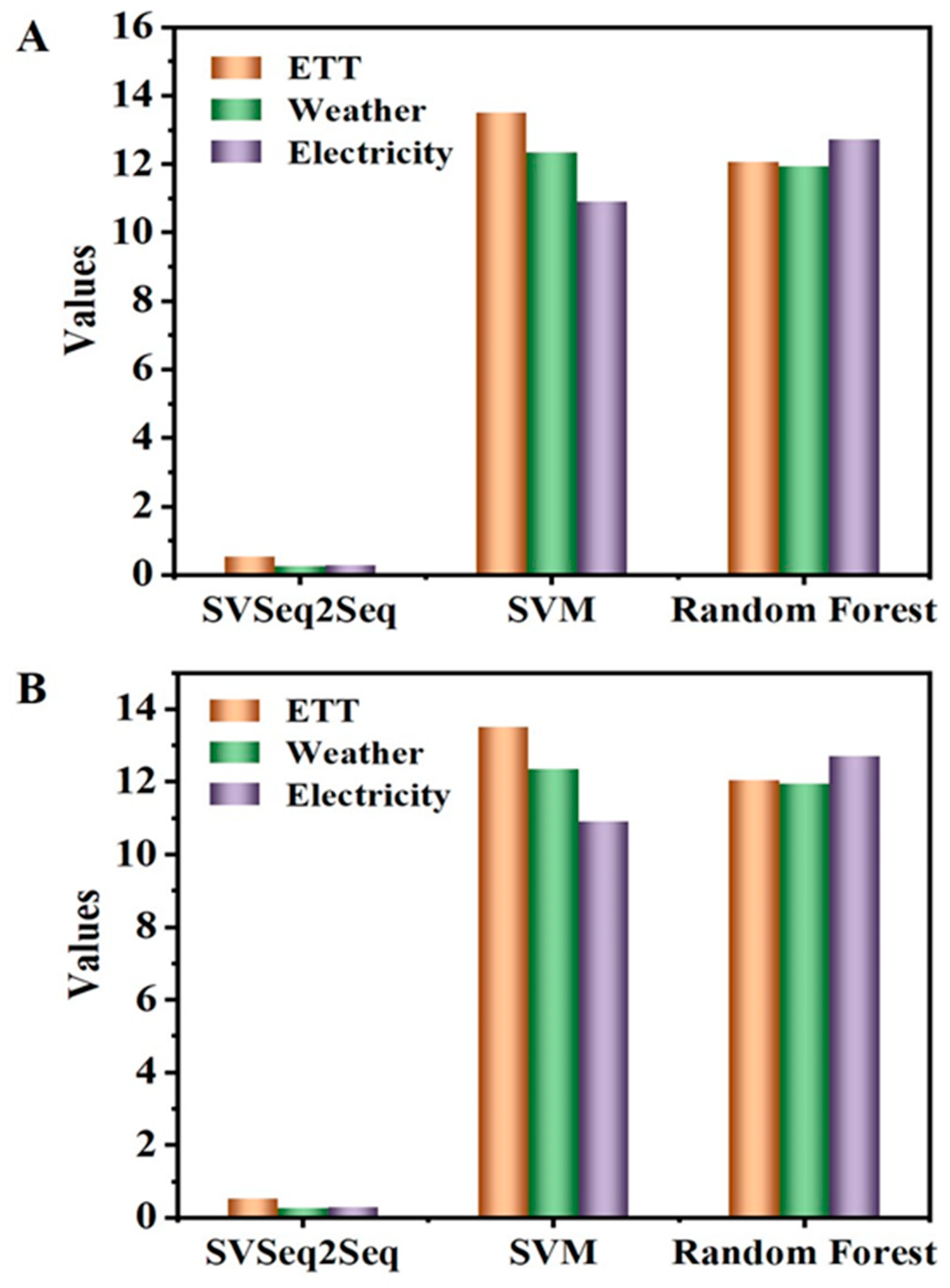
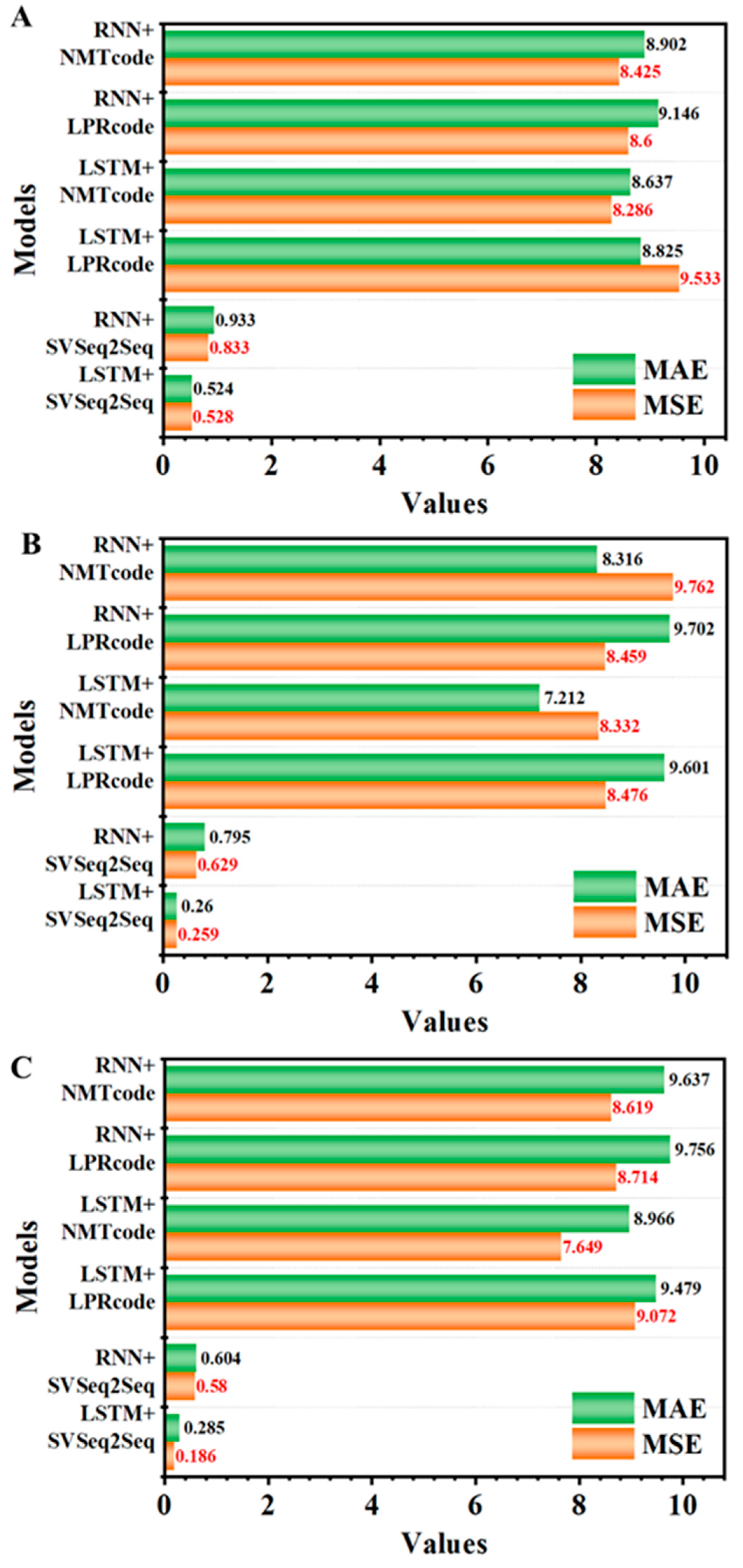
3.4. Comparison with Machine Learning-Based Methods

Traditional machine learning methods still hold advantages in sequence data forecasting. Therefore, we conduct extensive experiments to evaluate the forecasting performance of our proposed SVSeq2Seq model together with two conventional machine learning-based baselines, such as Support Vector Machines and Random Forest. As shown in

Table 1. The MSE and MAE values of the three models’ forecasting results.

Models	MSE 1			MAE 2
	SVSeq2Seq	SVM	RF	SVSeq2Seq	SVM	RF
ETT	0.528	12.971	14.562	0.524	13.518	12.057
Weather	0.259	14.732	11.604	0.260	12.351	11.943
Electricity	0.186	11.264	13.724	0.285	10.905	12.718

¹ Bold indicated the MSE optimal value; ² Bold indicated the MAE optimal value.

and Figure 4, our proposed SVSeq2Seq shows excellent prediction performance on the three datasets, both MSE and MAE, compared with the SVM and RF. In particular, the performance of the SVSeq2Seq model in the weather dataset was improved by 56.88 times in the weather dataset and 73.78 times in the electricity dataset at the MSE level, respectively.

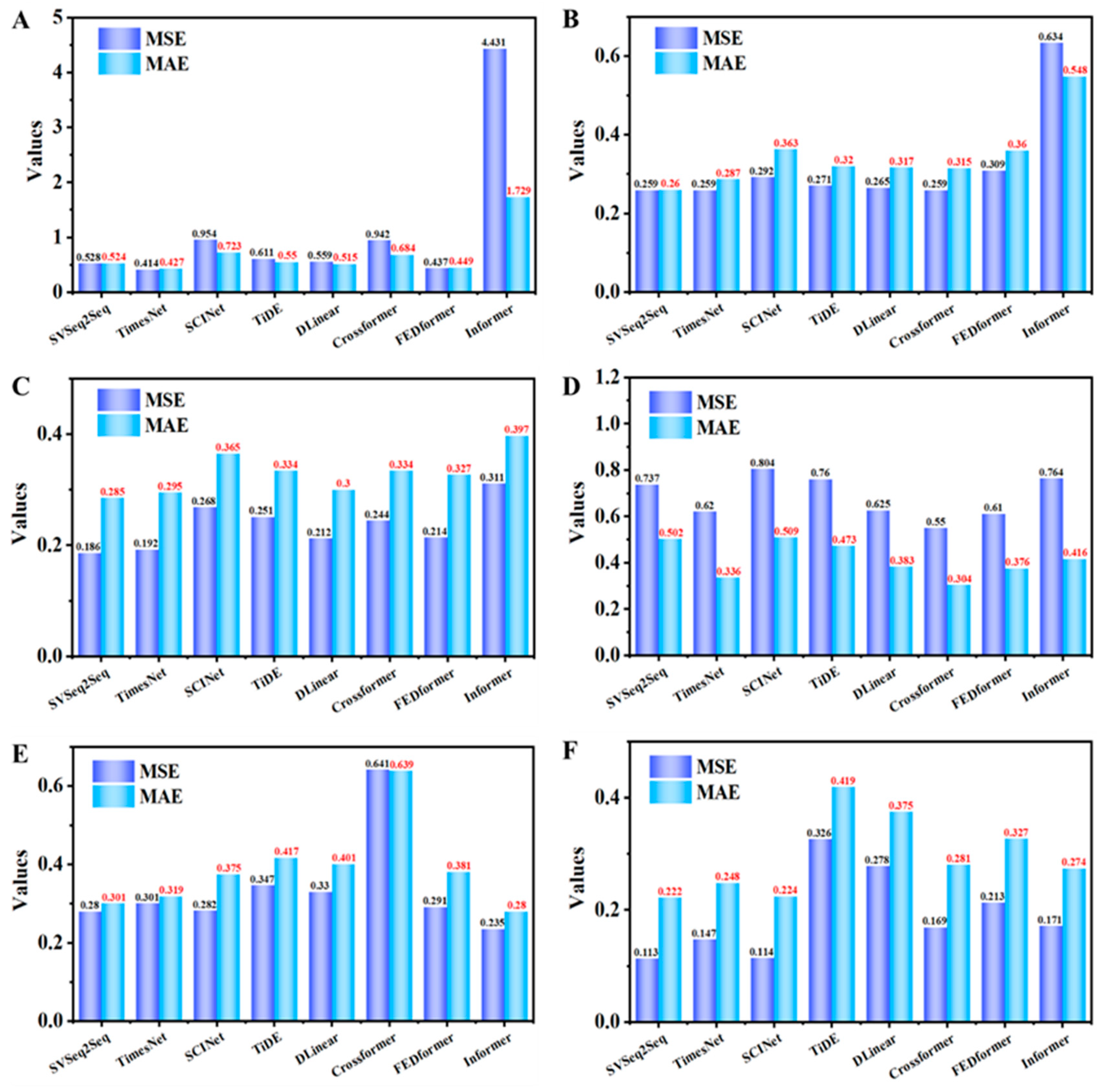
3.5. Comparison with Several Up-to-Date Methods

Further, we also compared our proposed model with several up-to-date methods, including Informer, FEDformer, Crossformer, DLinear, TiDE, SCINet, and TimesNet. The prediction results are shown in

Table 2. The MSE values of the eight models’ forecasting results.

Models	SVSeq2Seq	TimesNet	SCINet	TiDE	DLinear	Crossformer	FEDformer	Informer
ETT	0.528	0.414	0.954	0.611	0.559	0.942	0.437	4.431
Weather	0.259	0.259	0.292	0.271	0.265	0.259	0.309	0.634
Electricity	0.186	0.192	0.268	0.251	0.212	0.244	0.214	0.311
Traffic	0.737	0.620	0.804	0.760	0.625	0.550	0.610	0.764
Solar-Energy	0.280	0.301	0.282	0.347	0.330	0.641	0.291	0.235
PEMS	0.113	0.147	0.114	0.326	0.278	0.169	0.213	0.171

Bold indicated the MSE optimal value in different datasets.

and

Table 3. The MAE values of the eight models’ forecasting results.

Models	SVSeq2Seq	TimesNet	SCINet	TiDE	DLinear	Crossformer	FEDformer	Informer
ETT	0.524	0.427	0.723	0.550	0.515	0.684	0.449	1.729
Weather	0.260	0.287	0.363	0.320	0.317	0.315	0.360	0.548
Electricity	0.285	0.295	0.365	0.334	0.300	0.334	0.327	0.397
Traffic	0.502	0.336	0.509	0.473	0.383	0.304	0.376	0.416
Solar-Energy	0.301	0.319	0.375	0.417	0.401	0.639	0.381	0.280
PEMS	0.222	0.248	0.224	0.419	0.375	0.281	0.327	0.274

Bold indicated the MAE optimal value in different datasets.

, with the best results in bold. Lower MSE and MAE values indicate more accurate predictions. Our model outperforms other state-of-the-art baseline models on three out of the six datasets while achieving comparable results on the remaining three datasets. These results demonstrate the excellent performance of our model in sequence prediction scenarios.

As shown in Table 2, when evaluated using MSE as a metric, our proposed SVSeq2Seq model outperforms all other baseline models on the weather, electricity, and PEMS datasets. On the weather dataset, our proposed model performs comparable to TimesNet but outperforms Informer by up to 59.15%. On the electricity dataset, the SVSeq2Seq model we proposed performs up to 40.19% better than Informer. Similarly, the SVSeq2Seq model delivers up to 65.34% improvement over TiDE on the PEMS dataset.

When evaluated with MAE as the metric, the performance of the SVSeq2Seq model is essentially the same as when evaluated with MSE (Table 3). SVSeq2Seq shows an improvement of up to 52.55% over Informer in the weather dataset, up to 28.21% over Informer in the electricity dataset, and up to 47.01% over TiDE in the PEMS dataset.

Figure 5 illustrates the comparison of forecasting results between the SVSeq2Seq model and the other seven models on the ETT, weather, electricity, traffic, solar energy, and PEMS datasets. The results in Figure 5 show that the MSE and MAE of the SVSeq2Seq model exhibit significant advantages over the other seven baseline models in predicting the three datasets, i.e., weather, electricity, and PEMS. The MSE values are as low as 0.259, 0.186, and 0.113 in the weather, electricity, and PEMS datasets, respectively. Correspondingly, the MAE values were as low as 0.260, 0.285, and 0.222, respectively. In addition, the MAE and MSE values of the SVSeq2Seq model also perform well in the three other datasets, such as ETT, traffic, and solar energy. Therefore, our proposed SVSeq2Seq model displays exceptional forecasting ability in the six datasets.

3.6. Ablation Experiment

To verify the rationality and generality of our proposed state vector computation method, we performed detailed ablation experiments, including the replacement of different encoders, decoders, and state vector computation methods. LPRcode is a state vector computation method used in the reported study [3], where the output of the encoder is used as a direct input for the decoder. On the other hand, the reported NMTcode computes the state vector by summing the hidden states of the encoder [14]. The experimental results are shown in

Table 4. The MSE of the models’ forecasting results in ablation experiments.

Models	LSTM + SVSeq2Seq	RNN + SVSeq2Seq	LSTM + LPRcode	LSTM + NMTcode	RNN + LPRcode	RNN + NMTcode
ETT	0.528	0.833	9.533	8.286	8.600	8.425
Weather	0.259	0.629	8.476	8.332	8.459	9.762
Electricity	0.186	0.580	9.072	7.649	8.714	8.619

Bold indicated the MSE optimal value in different datasets.

and

Table 5. The MAE of the models’ forecasting results in ablation experiments.

Models	LSTM + SVSeq2Seq	RNN + SVSeq2Seq	LSTM + LPRcode	LSTM + NMTcode	RNN + LPRcode	RNN + NMTcode
ETT	0.524	0.933	8.825	8.637	9.146	8.902
Weather	0.260	0.795	9.601	7.212	9.702	8.316
Electricity	0.285	0.604	9.479	8.966	9.756	9.637

Bold indicated the MAE optimal value in different datasets.

.

The universality of the SVSeq2Seq model was confirmed in ablation experiments using MSE as the evaluation metric. To achieve this goal, LSTM and RNN were employed as encoders and decoders in sequential order. As shown in Table 4, the MSE of the ETT, weather, and electricity datasets exhibited minimal variations of 0.305, 0.37, and 0.304, respectively, demonstrating the robust universality of the SVSeq2Seq model. To provide additional evidence of the reliability of the SVSeq2Seq model, we also conducted a series of experiments using the LPRcode and NMTcode models, which resulted in a significant decrease in forecasting accuracy. Specifically, when LSTM was used as both the encoder and decoder on the ETT dataset, the MSE increased by 18.05 and 15.69 times, respectively. Similarly, when RNN was employed as both the encoder and decoder, the MSE increased by 10.32 times and 10.11 times, respectively. The significant increase in MSE after replacing SVSeq2Seq highlights the soundness of the proposed SVSeq2Seq model in the Sequence-to-Sequence framework.

The results of the ablation experiments were similar when using MAE as the evaluation metric and MSE as the benchmark. The chosen evaluation metrics did not appear to have a significant impact on the results. The LSTM and RNN were implemented sequentially as the encoder and decoder. Minor fluctuations in the MAE were observed on the ETT, weather, and electricity datasets, with values of 0.409, 0.535, and 0.319, correspondingly (Table 5). This confirms the superior adaptability of the SVSeq2Seq model. After replacing SVSeq2Seq with LPRcode and NMTcode, and using LSTM as both the encoder and decoder in the ETT dataset, MAE increased by 16.54 and 16.48 times, respectively. Similarly, when RNN was used as the encoder and decoder, the MAE increased by 9.8 folds and 9.5 times, respectively. These results affirm the effectiveness of the proposed SVSeq2Seq model.

Figure 6 shows the comparison of forecasting results for the ablation experiments in three real-world datasets, including ETT, weather, and electricity. As shown in Figure 6, regardless of whether LSTM or RNN is used as the encoder and decoder for the SVSeq2Seq model, the forecasting results are significantly superior to those obtained using LPRcode and NMTcode models. The above results indicate that the proposed SVSeq2Seq model has outstanding universality and rationality compared to the LPRcode and NMTcode models.

Furthermore, to validate the efficacy of the state vector, we eliminated all components of the state vector, such as SVSeq2Seq, LPRcode, and NMTcode. Compared with the proposed model with SVSeq2Seq as a state vector (Table 4 and Table 5), the MSE and MAE values of the model without state vector components increased substantially in both the LSTM and RNN models (

Table 6. The MSE and MAE of the models’ forecasting results.

Models	MSE 1		MAE 2
	LSTM	RNN	LSTM	RNN
ETT	9.603	10.492	9.548	10.734
Weather	8.972	9.776	9.670	9.809
Electricity	9.747	10.946	9.249	10.385

¹ Bold indicated the MSE optimal value; ² Bold indicated the MAE optimal value.

). These results demonstrated the significant contribution of the state vector, such as SVSeq2Seq, LPRcode, and NMTcode, within the Sequence-to-Sequence architecture.

4. Discussion

This study proposes an efficient method for computing state vectors in Sequence-to-Sequence architecture that can serve as a foundation for further research and development in sequence data forecasting. Even though we can mitigate the issue of gradient explosion and enhance the predictive performance of SVSeq2Seq by optimizing the computation of the state vector $c$ and employing tensor train, we still encountered numerous limitations and challenges during the early stages of modeling and development of SVSeq2Seq. Initially, computational and storage resources posed constraints on the model construction, hence we proposed the utilization of tensor train to alleviate this issue. Secondly, in terms of dataset selection, a significant amount of time was devoted to addressing the quality, quantity, and representativeness of the data. Lastly, the complexity of the model, hyperparameter tuning, interpretability, and the generalization ability of the SVSeq2Seq also presented considerable challenges throughout its development. After overcoming the above challenges, the SVSeq2Seq model has excellent performance in sequence data forecasting on multiple datasets.

Analyzing the above experimental results reveals that the SVSeq2Seq significantly outperforms traditional machine learning methods (e.g., SVM and RF) in the prediction of sequential data across ETT, weather, and electricity datasets. There are primarily two possible reasons for the suboptimal performance of machine learning algorithms in sequence prediction tasks. First, conventional SVMs and RFs do not inherently capture this sequential information as they assume the input features to be independent and identically distributed. This implies that without proper feature engineering to incorporate temporal information (such as using sliding windows, time lags, etc.), these models may fail to yield accurate predictions. Second, many sequence datasets exhibit non-linearities and non-stationarities. While RFs can capture a degree of non-linearity, they may not be sufficiently flexible for sequences with complex temporal dynamics. SVMs can address non-linearity issues by employing non-linear kernel functions, yet their predictive capacity might be compromised if the sequence data demonstrate significant non-stationarity.

In addition, our proposed SVSeq2Seq model still shows satisfactory performance compared with several up-to-date methods such as Informer, DLinear, and TimesNet in six real-world datasets. This observed significance can be attributed to the advantage of the tensor train network. A significant benefit of using a tensor train is that it is not affected by dimension enlargement. So, in practice, we can use a tensor train to approximate $f$. In SVSeq2Seq, we use the tensor train to reduce the parameter dimension from ${(q+k)}^{\mathrm{T}+1}$ to $(q+k)R^2(\mathrm{T}+1)$. This effectively reduces the amount of computation that increases sharply as $H^{extend}$ increases. Let $f\in {\mathcal{H}}_{\mu }^k$ be a Sobolev function defined on $\mathcal{I}=I_1\times I_2\times \cdots I_d$, where each $I_i$ is a set of vectors as given in Equation (14).

$${\mathcal{H}}_{\mathit{\mu }}^{\mathit{k}}=\left\{\mathit{f}\in {\mathit{L}}_{\mathit{\mu }}(\mathcal{I}):{\sum }_{\mathit{i}\le \mathit{k}}\hspace{0.17em}\parallel {\mathit{D}}^{\left(\mathit{i}\right)}\mathit{f}{\parallel }^{\mathbf{2}}<+\mathbf{\infty }\right\}$$

(14)

where $D^{\left(i\right)}f$ is i-th weak derivative of $f$ and $\mu \ge 0$. Any Sobolev function can be decomposed by Equation (15):

$$\mathit{f}(\cdot )={\sum }_{\mathbf{i}=\mathbf{0}}^{\mathbf{\infty }}\hspace{0.17em}\sqrt{\mathit{\lambda }\left(\mathit{i}\right)}\mathit{\gamma }(\cdot ;\mathit{i})\otimes \mathit{\varphi }(\mathit{i};\cdot )$$

(15)

where $\left\{\lambda \right\}$ is the eigenvalue and $\gamma \left(\right)$ and $\varphi \left(\right)$ are the eigenfunctions. Therefore, we will denote $f$ by Equation (16):

$$\mathit{f}\left(\mathbf{x}\right)={\sum }_{{\mathit{\alpha }}_{\mathbf{0}},\cdots ,{\mathit{\alpha }}_{\mathit{d}}=\mathbf{1}}^{\mathbf{\infty }}\hspace{0.17em}{\mathcal{A}}^{\mathbf{1}}({\mathit{\alpha }}_{\mathbf{0}},{\mathit{x}}_{\mathbf{1}},{\mathit{\alpha }}_{\mathbf{1}})\&\cdots {\mathcal{A}}^{\mathit{d}}({\mathit{\alpha }}_{\mathit{d}-\mathbf{1}},{\mathit{x}}_{\mathit{d}},{\mathit{\alpha }}_{\mathit{d}})$$

(16)

where $\left\{{\mathcal{A}}^d\right({\alpha }_{d-1},s_d,{\alpha }_d)=\sqrt{{\lambda }_{d-1}\left({\alpha }_{d-1}\right)}\varphi ({\alpha }_{d-1};s_d\left)\right\}$ is the basis function on each input dimension. Then, $f\left(\mathrm{x}\right)$ is truncated into a low-dimensional subspace $(\mathrm{r}<\mathbf{\infty })$ in Equation (17) as follows:

$$\mathit{f}\left(\mathbf{x}\right)={\sum }_{{\mathit{\alpha }}_{\mathbf{0}},\cdots ,{\mathit{\alpha }}_{\mathit{d}}}^{\mathbf{r}}\hspace{0.17em}{\mathcal{A}}^{\mathbf{1}}({\mathit{\alpha }}_{\mathbf{0}},{\mathit{x}}_{\mathbf{1}},{\mathit{\alpha }}_{\mathbf{1}})\cdots {\mathcal{A}}^{\mathit{d}}({\mathit{\alpha }}_{\mathit{d}-\mathbf{1}},{\mathit{x}}_{\mathit{d}},{\mathit{\alpha }}_{\mathit{d}})$$

(17)

5. Conclusions

In this paper, we propose a novel and efficient state vector calculation method for Sequence-to-Sequence architecture forecasting, in which the proposed SVSeq2Seq model uses the correlation between the hidden layers of the decoder and the encoder to compute the weight vector of the hidden layer of the encoder. It is worth noting that as the number of hidden layers in the encoder increases, the computational complexity of this method grows exponentially. In addition, we introduce the use of tensor train decomposition to approximate the extended tensor, which effectively mitigates the curse of the dimensionality problem. The experimental results demonstrate that the proposed SVSeq2Seq outperforms the reported baseline models in most scenarios. When using the MSE as an evaluation metric, the SVSeq2Seq model achieved the best results with scores of 0.259, 0.186, and 0.113 on the weather, electricity, and PEMS datasets, respectively. With the MAE as the evaluation metric, SVSeq2Seq obtained optimal results with scores of 0.260, 0.285, and 0.222 on the datasets, respectively, demonstrating the effectiveness of SVSeq2Seq in sequence prediction tasks. In the ablation experiment, regardless of whether MSE or MAE was used as the evaluation criterion, the SVSeq2Seq group achieved the best performance on the ETT, weather, and electricity datasets, indicating that our model possesses excellent generalizability. The experimental results demonstrate that SVSeq2Seq exhibits superior performance in sequence data prediction tasks, particularly in predicting long-term nonlinear sequence data. In the future, we plan to further enhance the flow of data within the encoder and decoder, and optimize the computation of memory information weights within the RNN to improve the sequence prediction capabilities of SVSeq2Seq. Regarding machine learning approaches, we will explore the use of ensemble learning techniques in conjunction with hyperparameter tuning to enhance the performance of machine learning methods in sequence prediction tasks. Additionally, we aim to further investigate the application of the state vector in time series analysis tasks using Transformer-based methods.

References

1. Barbosa, A.; Bittencourt, I.; Siqueira, S.W.; Dermeval, D.; Cruz, N.J.T. A context-independent ontological linked data alignment approach to instance matching. Int. J. Semant. Web. Inf. 2022, 18, 1–29. [Google Scholar] [CrossRef]
2. Hochreiter, S.; Schmidhuber, J. Long short-term memory. Neural Comput. 2010, 9, 1735–1780. [Google Scholar] [CrossRef] [PubMed]
3. Cho, K.; Merrienboer, B.V.; Gulcehre, C.; Bahdanau, D.; Bougares, F.; Schwenk, H.; Bengio, Y. Learning phrase representations using RNN encoder-decoder for statistical machine translation. In Proceedings of the 2014 Conference on Empirical Methods in Natural Language Processing, Doha, Qatar, 25–29 October 2014; Volume 1406, p. 1078. [Google Scholar] [CrossRef]
4. Wu, H.; Xu, J.; Wang, J.; Long, M. Autoformer: Decomposition transformers with auto-correlation for long-term series forecasting. In Proceedings of the 35th Conference on Neural Information Processing Systems, Online, 6–14 December 2021; pp. 22419–22430. [Google Scholar] [CrossRef]
5. Zhang, Y.; Yan, J. Crossformer: Transformer utilizing cross-dimension dependency for multivariate time series forecasting. In Proceedings of the Eleventh International Conference on Learning Representations, Kigali, Rwanda, 1–5 May 2023. [Google Scholar] [CrossRef]
6. Zeng, A.; Chen, M.; Zhang, L.; Xu, Q. Are transformers effective for time series forecasting? In Proceedings of the AAAI Conference on Artificial Intelligence, Washington, DC, USA, 7–14 February 2023. [Google Scholar] [CrossRef]
7. Das, A.; Kong, W.; Leach, A.; Mathur, S.; Sen, R.; Yu, R. Long-term forecasting with TiDE: Time-series dense encoder. Trans. Mach. Learn. Res. 2023, 2304, 08424. [Google Scholar] [CrossRef]
8. Liu, M.; Zeng, A.; Chen, M.; Xu, Z.; Lai, Q.; Ma, L.; Xu, Q. Scinet: Time series modeling and forecasting with sample convolution and interaction. In Proceedings of the 36th Conference on Neural Information Processing Systems, New Orleans, LA, USA, 28 November–9 December 2022; Volume 35, pp. 5816–5828. [Google Scholar] [CrossRef]
9. Wu, H.; Hu, T.; Liu, Y.; Zhou, H.; Wang, J.; Long, M. Timesnet: Temporal 2d-variation modeling for general time series analysis. In Proceedings of the Eleventh International Conference on Learning Representations, Virtual Event, 25–29 April 2022; Volume 2210, p. 02186. [Google Scholar] [CrossRef]
10. Zhou, H.; Zhang, S.; Peng, J.; Zhang, S.; Li, J.; Xiong, H.; Zhang, W. Informer: Beyond efficient transformer for long sequence time-series forecasting. In Proceedings of the AAAI Conference on Artificial Intelligence, Held Virtually, 2–9 February 2021. [Google Scholar] [CrossRef]
11. Li, C.; Li, D.; Zhang, Z.; Chu, D. MST-RNN: A multi-dimension spatiotemporal recurrent neural networks for recommending the next point of interest. Mathematics 2022, 10, 1838. [Google Scholar] [CrossRef]
12. Sneha, J.; Zhao, J.; Fan, Y.; Li, J.; Lin, H.; Yan, C.; Chen, M. Time-varying sequence model. Mathematics 2023, 11, 336. [Google Scholar] [CrossRef]
13. Sutskever, I.; Vinyals, O.; Le, Q.V. Sequence to sequence learning with neural networks. In Proceedings of the 27th International Conference on Neural Information Processing Systems (NeurIPS 2014), Montreal, QC, Canada, 8–13 December 2014. [Google Scholar] [CrossRef]
14. Rico, S.; Haddow, B.; Birch, A. Neural machine translation of rare words with subword units. In Proceedings of the 54th Annual Meeting of the Association for Computational Linguistics, Berlin, Germany, 7–12 August 2016. [Google Scholar] [CrossRef]
15. Serban, I.V.; Sordoni, A.; Bengio, Y.; Courville, A.; Pineau, J. Building end-to-end dialogue systems using generative hierarchical neural network models. AAAI Conf. Artif. Intell. 2016, 1410, 3916. [Google Scholar] [CrossRef]
16. Sordoni, A.; Bengio, Y.; Vahabi, H.; Lioma, C.; Simonsen, J.G.; Nie, J. A hierarchical recurrent encoder-decoder for generative context-aware query suggestion. In Proceedings of the 24th ACM International on Conference on Information and Knowledge Management, Melbourne, Australia, 19–23 October 2015; pp. 553–562. [Google Scholar] [CrossRef]
17. Serban, I.V.; Sordoni, A.; Lowe, R.; Charlin, L.; Pineau, J.; Courville, A.; Bengio, Y. A hierarchical latent variable encoder-decoder model for generating dialogues. In Proceedings of the AAAI Conference on Artificial Intelligence, San Francisco, CA, USA, 4–9 February 2017. [Google Scholar] [CrossRef]
18. Jason, W.; Chopra, S.; Bordes, A. Memory networks. In Proceedings of the 30th ACM International Conference on Multimedia, Lisboa, Portugal, 10–14 October 2022; pp. 7380–7382. [Google Scholar] [CrossRef]
19. Fernando, T.; Denman, S.; McFadyen, A.; Sridharan, S.; Fookes, C. Tree memory networks for modelling long-term temporal dependencies. Neurocomputing 2018, 304, 64–81. [Google Scholar] [CrossRef]
20. Cao, J.; Li, J.; Jiang, J. Link prediction for temporal heterogeneous networks based on the information lifecycle. Mathematics 2023, 11, 3541. [Google Scholar] [CrossRef]
21. Brown, T.B.; Mann, B.; Ryder, N.; Subbiah, M.; Kaplan, J.; Dhariwal, P.; Neelakantan, A.; Shyam, P.; Sastry, G.; Askell, A.; et al. Language models are few-shot learners. In Proceedings of the 34th International Conference on Neural Information Processing Systems, Online, 6–12 December 2020; Volume 33, pp. 1877–1901. [Google Scholar] [CrossRef]
22. Dosovitskiy, A.; Beyer, L.; Kolesnikov, A.; Weissenborn, D.; Zhai, X.; Unterthiner, T.; Dehghani, M.; Minderer, M.; Heigold, G.; Gelly, S.; et al. An image is worth 16×16 words: Transformers for image recognition at scale. arXiv 2021, arXiv:2010.11929. [Google Scholar] [CrossRef]
23. Liu, Y.; Wu, H.; Wang, J.; Long, M. Non-stationary transformers: Rethinking the stationarity in time series forecasting. arXiv 2022, arXiv:2205.14415. [Google Scholar] [CrossRef]
24. Nie, Y.; Nguyen, N.H.; Sinthong, P.; Kalagnanam, J. A time series is worth 64 words: Long-term forecasting with transformers. arXiv 2022, arXiv:2211.14730. [Google Scholar] [CrossRef]
25. Singh, S.K.; Chopra, M.; Sharma, A.; Gill, S.S. A comparative study of generative adversarial networks for text-to-image synthesis. Int. J. Softw. Sci. Comp. 2022, 14, 1–12. [Google Scholar] [CrossRef]
26. Román, O. A practical introduction to tensor networks: Matrix product states and projected entangled pair states. Ann. Phys. 2014, 349, 117–158. [Google Scholar] [CrossRef]
27. Zhou, T.; Ma, Z.; Wen, Q.; Wang, X.; Sun, L.; Jin, R. Fedformer: Frequency enhanced decomposed transformer for long-term series forecasting. Int. Conf. Mach. Learn. 2022, 2201, 12740. [Google Scholar] [CrossRef]
28. Lai, G.; Chang, W.C.; Yang, Y.; Liu, H. Modeling long-and short-term temporal patterns with deep neural networks. In Proceedings of the 41st International ACM SIGIR Conference on Research & Development in Information Retrieval, Ann Arbor, MI, USA, 8–12 July 2018; pp. 95–104. [Google Scholar] [CrossRef]
Figure 1. The operational status of SVseq2seq within the Sequence-to-Sequence structure.
Mathematics 12 00265 g001
Figure 2. The computation procedure of the state vector c .
Mathematics 12 00265 g002
Figure 3. Schematic diagram of the working of tensor train networks.
Mathematics 12 00265 g003
Figure 4. Comparison of the forecasting results of the SVSeq2Seq model with SVM and RF at the MSE (A) and MAE (B) level on three real-world datasets.
Mathematics 12 00265 g004
Figure 5. Comparison of the forecasting results of the SVSeq2Seq model with other models on six real-world datasets. (A) ETT dataset; (B) weather dataset; (C) electricity dataset; (D) traffic dataset; (E) solar energy dataset; (F) PEMS dataset. The black and red colors of numbers indicated the MSE and MAE values, respectively.
Mathematics 12 00265 g005
Figure 6. Comparison of forecasting results for ablation experiments in three real-world datasets. (A) ETT dataset; (B) weather dataset; (C) electricity dataset. The black and red colors of numbers indicated the MAE and MSE values, respectively.
Mathematics 12 00265 g006