Chaotic Binarization Schemes for Solving Combinatorial Optimization Problems Using Continuous Metaheuristics

Cisternas-Caneo, Felipe; Crawford, Broderick; Soto, Ricardo; Giachetti, Giovanni; Paz, Álex; Peña Fritz, Alvaro

doi:10.3390/math12020262

Open AccessArticle

Chaotic Binarization Schemes for Solving Combinatorial Optimization Problems Using Continuous Metaheuristics

¹

Escuela de Ingeniería Informática, Pontificia Universidad Católica de Valparaíso, Avenida Brasil 2241, Valparaíso 2362807, Chile

²

Facultad de Ingeniería, Universidad Andres Bello, Antonio Varas 880, Providencia, Santiago 7591538, Chile

³

Escuela de Ingeniería de Construcción y Transporte, Pontificia Universidad Católica de Valparaíso, Avenida Brasil 2147, Valparaíso 2362804, Chile

^*

Authors to whom correspondence should be addressed.

Mathematics 2024, 12(2), 262; https://doi.org/10.3390/math12020262

Submission received: 30 November 2023 / Revised: 22 December 2023 / Accepted: 8 January 2024 / Published: 12 January 2024

(This article belongs to the Special Issue Mathematical Optimization and Decision Making Analysis)

Download

Browse Figures

Versions Notes

Abstract

:

Chaotic maps are sources of randomness formed by a set of rules and chaotic variables. They have been incorporated into metaheuristics because they improve the balance of exploration and exploitation, and with this, they allow one to obtain better results. In the present work, chaotic maps are used to modify the behavior of the binarization rules that allow continuous metaheuristics to solve binary combinatorial optimization problems. In particular, seven different chaotic maps, three different binarization rules, and three continuous metaheuristics are used, which are the Sine Cosine Algorithm, Grey Wolf Optimizer, and Whale Optimization Algorithm. A classic combinatorial optimization problem is solved: the 0-1 Knapsack Problem. Experimental results indicate that chaotic maps have an impact on the binarization rule, leading to better results. Specifically, experiments incorporating the standard binarization rule and the complement binarization rule performed better than experiments incorporating the elitist binarization rule. The experiment with the best results was STD_TENT, which uses the standard binarization rule and the tent chaotic map.

Keywords:

chaotic maps; binarization schemes; knapsack problem; Sine Cosine Algorithm; Grey Wolf Optimizer; Whale Optimization Algorithm

MSC:

90C27

1. Introduction

Optimization problems are increasingly relevant across a wide range of sectors, including mining, energy, telecommunications, and health. A prominent type of these problems is combinatorial optimization problems, where the decision variables are of a categorical nature, such as binary. In these cases, the challenge is to identify the best possible combination of these variables.

The complexity of solving these problems increases exponentially with the number of decision variables. This is because, in a binary combinatorial problem, the search space of these problems is

2^{n}

, where n represents the total number of decision variables. This exponential growth of the search space poses significant computational and analytical challenges.

According to the literature [1], methods for addressing complex optimization problems are classified into two main categories: exact methods and approximate methods.

Exact Methods: These methods focus on ensuring an optimal solution by exhaustively exploring the entire search space. However, their applicability is limited due to scalability issues. As the complexity of the problem increases, the time required to find an optimal solution increases significantly, which can make them impractical for large-scale problems or those with an excessively large search space.
Approximate Methods: Unlike exact methods, approximate methods do not guarantee the attainment of an optimal solution. However, they are capable of providing high-quality solutions within reasonable computational times, making them very valuable in practice, especially for complex and large-scale problems. Within this category, metaheuristics are particularly notable. These techniques, which include Genetic Algorithms (GA), Particle Swarm Optimization (PSO), and Ant Colony Optimization (ACO), are known for their ability to find efficient solutions to complex problems through intelligent exploration of the search space, avoiding getting trapped in sub-optimal local solutions.

Thus, exact methods are ideal for smaller, manageable problems where precision is required, whereas approximate methods, especially metaheuristics, are the preferred option for larger-scale problems or those with time constraints, where a ”good enough” solution is acceptable and often necessary.

The study of metaheuristics has grown in recent years, with hybridizations emerging as the current trend. There exist hybridizations between metaheuristics such as those proposed in [2,3,4,5], hyperheuristic approaches where a high-level metaheuristic guides another low-level one [6,7,8], approaches where machine learning techniques enhance metaheuristics [9,10,11], and other approaches in which chaos theory is utilized to modify the stochastic behavior of metaheuristics [12,13,14,15].

The integration of chaotic maps into metaheuristics has caught the attention of the scientific community due to its advantages, such as low computational cost and rapid adaptability [16]. Chaotic maps are used as generators of random sequences, contributing to an improvement in the stochastic behavior of metaheuristics. This approach is utilized in various aspects of metaheuristics such as the initialization of solutions [17,18] or in the solution perturbation operators [19,20]. The hybridization of metaheuristics with chaotic maps is significant because it enhances the ability of metaheuristics to avoid getting trapped in local minima and improves global exploration of the search space.

In reviewing the different metaheuristics existing in the literature [21], we can observe that most of them are designed to solve continuous problems; therefore, to solve binary combinatorial problems, it is necessary to binarize them. According to the literature [22], there are different ways to binarize metaheuristics, among which the two-step technique stands out. This binarization process is carried out in two steps: (1) applying a transfer function and (2) applying a binarization rule. In the present work, chaotic maps were used to change the stochastic behavior of the binarization rule to binarize continuous metaheuristics. Specifically, seven chaotic maps were used, which were compared with the original stochastic behavior for binarizing three metaheuristics widely used in the literature.

Among the great variety of metaheuristics that exist in the literature, in the present work we chose the Sine Cosine Algorithm (SCA) [23], Grey Wolf Optimizer (GWO) [24], and Whale Optimization Algorithm (WOA) [25]. These three metaheuristics are population metaheuristics designed to solve continuous optimization problems of great interest to the scientific community. This interest is reflected in the use of these metaheuristics in different works where, for example, SCA was used in [26,27,28,29,30,31], GWO was used in [32,33,34,35,36,37,38,39], and WOA was used in [40,41,42,43,44,45,46].

Given this great interest, the good results obtained in different optimization problems, and the No Free Lunch Theorem [47,48], we are motivated to investigate the behavior of these three metaheuristics in a combinatorial optimization problem, the Knapsack Problem, with the hybridization of chaotic maps.

The main contributions of this work are the following:

Incorporate chaotic maps into binarization schemes to develop chaotic binarization schemes.
Use these chaotic binarization schemes in three continuous metaheuristics to solve the 0-1 Knapsack Problem.
Analyze the results obtained in terms of descriptive statistics, convergence, and non-parametric statistical test.

The following is a brief summary of the structure of this paper: Section 2 provides a comprehensive review of related works that utilize continuous metaheuristics (Section 2.1), defines chaotic maps (Section 2.2), and assesses their application in metaheuristics (Section 2.3). Section 3 examines how continuous metaheuristics can be leveraged to solve binary combinatorial optimization problems. Section 4 outlines our research proposal, which focuses on the implementation of chaotic binarization schemes. Section 5 of this paper details the 0-1 Knapsack Problem (Section 5.1), the experiment configuration (Section 5.2), the results analysis (Section 5.3), the algorithm convergence analysis (Section 5.4), and the non-parametric statistical test analysis (Section 5.5). Finally, Section 6 presents conclusions and future work.

2. Related Work

2.1. Metaheuristics

Metaheuristics are highly flexible and efficient algorithms, capable of delivering quality solutions in manageable computational times [1]. The efficacy of metaheuristics is largely due to their ability to balance two critical phases in the search process, diversification (or exploration) and intensification (or exploitation), using specific operators that vary according to the algorithm in question.

The development of metaheuristics, stimulated by the No Free Lunch Theorem [47,48,49], is based on a variety of sources of inspiration, including human behavior, genetic evolution, social interactions among animals, and physical phenomena. This theorem, fundamental in the field of optimization, states that there is no universal algorithm that is most efficient for solving all optimization problems. The following section will introduce and define the three metaheuristics employed in this research.

2.1.1. Sine Cosine Algorithm

The Sine Cosine Algorithm (SCA) is a metaheuristic proposed by Mirjalili in 2016 [23]. This metaheuristic was designed to solve continuous optimization problems and is inspired by the dual behavior of the trigonometric functions sine and cosine. Algorithm 1 presents the behavior of SCA.

2.1.2. Grey Wolf Optimizer

The Grey Wolf Optimizer [24], proposed by Mirjalili in 2014, is a metaheuristic inspired by the hunting behavior and hierarchical social structure of the grey wolf. The efficacy of this technique is based on the imitation of the dynamics and social interactions observed in a pack of wolves.

In a wolf pack, there are four types of hierarchical roles that are essential in the structure of the GWO.

Alpha ( $α$ ): These are the wolves that lead the pack. In the context of GWO, they represent the current best solution. The alpha guides the search process and decision making during optimization.
Beta ( $β$ ): These wolves support the alpha and are considered the second-best solution. In the metaheuristic, they assist in directing the search, providing a secondary perspective in the solution space.
Delta ( $δ$ ): Though strong, delta wolves lack leadership skills. They are the third-best solution in the optimization process and contribute to the diversity of the search, bringing variability and preventing the pack (the algorithm) from becoming stagnant.
Omega ( $ω$ ): These wolves are the lowest in the social hierarchy. They have no leadership power and are dedicated to following and protecting the younger members of the pack. In GWO, they represent the other possible solutions, following the lead of the higher-ranking wolves.

Algorithm 1 Sine Cosine Algorithm

Input: The population

X =

{X_{1}, X_{2}, \dots, X_{i}}

Output: The updated population

X^{'} =

{X_{1}^{'}, X_{2}^{'}, \dots, X_{i}^{'}}

and

X_{b e s t}

1:: Initialize random population X
2:: Evaluate the objective function of each individual in the population X
3:: Identify the best individual in the population ( $X_{b e s t}$ )
4:: a = 2
5:: for $i t e r a t i o n (t)$ do
6:: $r_{1} = a - (t \cdot (a / m a x I t e r))$
7:: for $s o l u t i o n (i)$ do
8:: for $d i m e n s i o n (j)$ do
9:: $r a n d = r a n d (0, 1)$
10:: $r_{2} = (2 \cdot π) \cdot r a n d (0, 1)$
11:: $r a n d = r a n d (0, 1)$
12:: $r_{3} = 2 \cdot r a n d (0, 1)$
13:: $r_{4} = r a n d (0, 1)$
14:: if $r_{4} < 0.5$ then
15:: $X_{i, j}^{t} = X_{i, j}^{t} + (r_{1} \cdot s i n (r_{2}) \cdot | r_{3} \cdot X_{b e s t, j} - X_{i, j}^{t} |)$
16:: else
17:: $X_{i, j}^{t} = X_{i, j}^{t} + (r_{1} \cdot c o s (r_{2}) \cdot | r_{3} \cdot X_{b e s t, j} - X_{i, j}^{t} |)$
18:: end if
19:: end for
20:: end for
21:: Evaluate the objective function of each individual in the population X
22:: Update $X_{b e s t}$
23:: end for
24:: Return the updated population X where $X_{b e s t}$ is the best result

The implementation of these hierarchies in the GWO allows the algorithm to effectively balance exploration (diversification) and exploitation (intensification) of the solution space. The inspiration from the behavior and social structure of grey wolves brings a unique methodology for solving complex optimization problems. Algorithm 2 presents the behavior of GWO.

2.1.3. Whale Optimization Algorithm

The Whale Optimization Algorithm (WOA) is a metaheuristic developed by Mirjalili and Lewis in 2016 [25], inspired by the hunting behavior and social structure of whales. This algorithm mimics the hunting strategy known as “bubble-net feeding”, a sophisticated and coordinated method used by whales to capture their prey. The WOA is characterized by three main phases in its search and optimization process:

Search for the prey: The whales (search agents) explore the solution space to locate the prey (the best solution). Notably in WOA, unlike other metaheuristics, the position update of each search agent is based on a randomly selected agent, not necessarily the best one found so far. This allows for a broader and more diversified exploration of the solution space.
Encircling the prey: Once the prey (best solution) is identified, the whales position themselves to encircle it. This stage represents an intensification phase, where the algorithm concentrates on the area around the promising solution identified in the search phase.
Bubble-net attacking: In the final phase, the whales attack the prey using the bubble-net technique. This phase represents a coordinated and focused effort to refine the search in the selected region and optimize the solution.

Algorithm 2 Grey Wolf Optimizer

Input: The population

X =

{X_{1}, X_{2}, \dots, X_{i}}

Output: The updated population

X^{'} =

{X_{1}^{'}, X_{2}^{'}, \dots, X_{i}^{'}}

and

X_{b e s t}

1:: Initialize random population X
2:: Evaluate the objective function of each individual in the population X
3:: Identify the best individual in the population ( $X_{b e s t}$ )
4:: for $i t e r a t i o n (t)$ do
5:: a = 2 − t · (2/maxIter)
6:: Determine alpha wolf ( $X_{a l p h a}$ ) ▹ $X_{a l p h a}$ is the best solution
7:: Determine beta wolf ( $X_{b e t a}$ ) ▹ $X_{b e t a}$ is the second best solution
8:: Determine delta wolf ( $X_{d e l t a}$ ) ▹ $X_{d e l t a}$ is the third best solution
9:: for $s o l u t i o n (i)$ do
10:: for $d i m e n s i o n (j)$ do
11:: $r_{1}$ = rand(0,1)
12:: $r_{2}$ = rand(0,1)
13:: $A_{1}$ = $2 \cdot a \cdot r_{1} - a$
14:: $C_{1}$ = $2 \cdot r_{2}$
15:: $d_{a l p h a} = | (C_{1} \cdot X_{a l p h a, j}^{t}) - X_{i, j}^{t} |$
16:: $X_{1} = X_{a l p h a, j}^{t} - (A_{1} \cdot d_{a l p h a})$
17:: $r_{1}$ = rand(0,1)
18:: $r_{2}$ = rand(0,1)
19:: $A_{2}$ = $2 \cdot a \cdot r_{1} - a$
20:: $C_{2}$ = $2 \cdot r_{2}$
21:: $d_{b e t a} = | (C_{2} \cdot X_{b e t a, j}^{t}) - X_{i, j}^{t} |$
22:: $X_{2} = X_{b e t a, j}^{t} - (A_{2} \cdot d_{b e t a})$
23:: $r_{1}$ = rand(0,1)
24:: $r_{2}$ = rand(0,1)
25:: $A_{3}$ = $2 \cdot a \cdot r_{1} - a$
26:: $C_{3}$ = $2 \cdot r_{2}$
27:: $d_{d e l t a} = | (C_{3} \cdot X_{d e l t a, j}^{t}) - X_{i, j}^{t} |$
28:: $X_{3} = X_{d e l t a, j}^{t} - (A_{3} \cdot d_{d e l t a})$
29:: $X_{i, j}^{t} = (X_{1} + X_{2} + X_{3}) / 3$
30:: end for
31:: end for
32:: Evaluate the objective function of each individual in the population X
33:: Update $X_{b e s t}$
34:: end for
35:: Return the updated population X where $X_{b e s t}$ is the best result

The structure of these phases enables the WOA to effectively balance between exploration and exploitation, making it suitable for solving a wide range of complex optimization problems. Algorithm 3 presents the behavior of WOA.

2.2. Chaotic Maps

Dynamic systems, characterized by their lack of linearity and periodicity, exhibit chaos in a way that is both deterministic and seemingly random [50]. Such a characteristic of the dynamic system is recognized as a generator of random behaviors [51]. It is crucial to understand that chaos, although it follows specific patterns and is based on chaotic variables, is not synonymous with absolute randomness [52]. The implementation of chaotic mappings is valued for its ability to minimize computational costs and because it requires only a limited set of initial parameters [16].

Chaotic behavior demonstrates high sensitivity to variations in initial conditions, meaning that any modification of these conditions will influence the resulting sequence [53]. There are numerous chaotic maps referenced in the scientific literature, of which ten are of special relevance [50,52,54]. 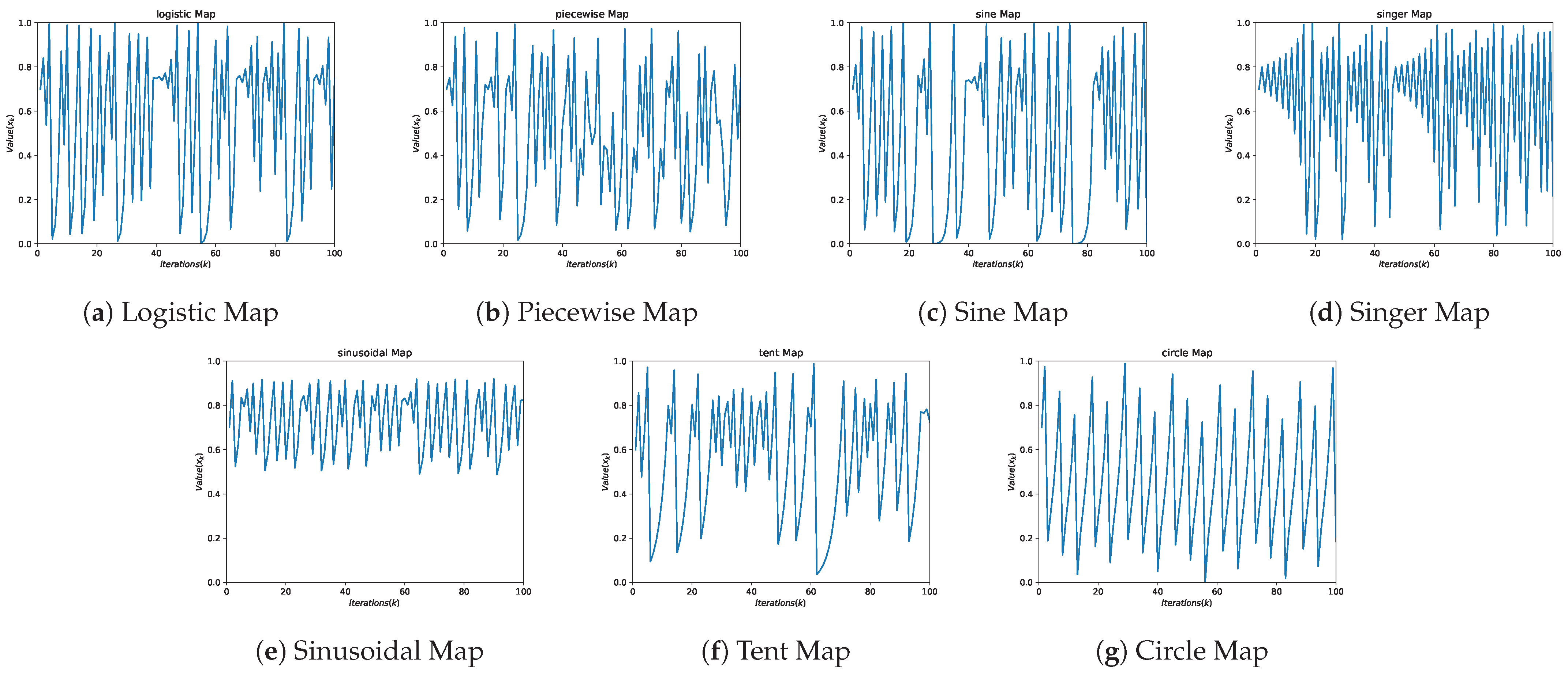Equations (1)–(7) shows seven of these chaotic maps, and Figure 1 details the behavior of each of the previously mentioned chaotic maps.

Algorithm 3 Whale Optimization Algorithm

Input: The population

X =

{X_{1}, X_{2}, \dots, X_{i}}

Output: The updated population

X^{'} =

{X_{1}^{'}, X_{2}^{'}, \dots, X_{i}^{'}}

and

X_{b e s t}

1:: Initialize random population X
2:: Evaluate the objective function of each individual in the population X
3:: Identify the best individual in the population ( $X_{b e s t}$ )
4:: $b = 1$
5:: for $i t e r a t i o n (t)$ do
6:: $a = 2 - ((2 \cdot t) / m a x I t e r)$
7:: for $s o l u t i o n (i)$ do
8:: $p = r a n d (0, 1)$
9:: $r a n d = r a n d (0, 1)$
10:: $A = 2 \cdot a \cdot (r a n d - a$
11:: $r a n d = r a n d (0, 1)$
12:: $C = 2 \cdot r a n d$
13:: $l = r a n d (- 1, 1)$
14:: if $p < 0.5$ then
15:: if $| A | < 1$ then
16:: for $d i m e n s i o n (j)$ do
17:: $D = | (C \cdot X_{b e s t, j}) - X_{i, j}^{t} |$
18:: $X_{i, j}^{t} = X_{b e s t, j} - (A \cdot D)$
19:: end for
20:: else
21:: $X_{r a n d o m} =$ random individual from the population
22:: for $d i m e n s i o n (j)$ do
23:: $D = | (C \cdot X_{r a n d o m, j}) - X_{i, j}^{t} |$
24:: $X_{i, j}^{t} = X_{r a n d o m, j} - (A \cdot D)$
25:: end for
26:: end if
27:: else
28:: for $d i m e n s i o n (j)$ do
29:: $D^{^{'}} = X_{b e s t, j} - X_{i, j}^{t}$
30:: $X_{i, j}^{t} = (D^{^{'}} \cdot e^{b \cdot l} \cdot c o s (2 \cdot π \cdot l)) + X_{b e s t, j}$
31:: end for
32:: end if
33:: end for
34:: Evaluate the objective function of each individual in the population X
35:: Update $X_{b e s t}$
36:: end for
37:: Return the updated population X where $X_{b e s t}$ is the best result

L o g i s t i c M a p ⟶ x_{k + 1} = c \cdot x_{k} (1 - x_{k}), c = 4

(1)

P i e c e w i s e M a p ⟶ x_{k + 1} = \{\begin{matrix} \frac{x_{k}}{l} & 0 \leq x_{k} < l \\ \frac{x_{k} - l}{0.5 - l} & l \leq x_{k} < 0.5 \\ \frac{1 - l - x_{k}}{0.5 - l} & 0.5 \leq x_{k} < 1 - l \\ \frac{1 - x_{k}}{l} & 1 - l \leq x_{k} < 1 \end{matrix}, l = 0.4

(2)

S i n e M a p ⟶ x_{k + 1} = \frac{c}{4} s i n (π x_{k}), c = 4

(3)

S i n g e r M a p ⟶ μ (7.86 x_{k} - 23.31 x_{k}^{2} + 23.75 x_{k}^{3}) - 13.302875 x_{k}^{4}, μ = 1.07

(4)

S i n u s o i d a l M a p ⟶ x_{k + 1} = c x_{k}^{2} s i n (π x_{k}), c = 2.3

(5)

T e n t M a p ⟶ x_{k + 1} = \{\begin{matrix} \frac{x_{k}}{0.7} & x_{k} < 0.7 \\ \frac{10}{3} (1 - x_{k}) & x_{k} \geq 0.7 \end{matrix}

(6)

C i r c l e M a p ⟶ x_{k + 1} = m o d (x_{k} + d - (\frac{c}{2 π}) \cdot s i n (2 π x_{k} >), 1), c = 0.5 a n d d = 0.2

(7)

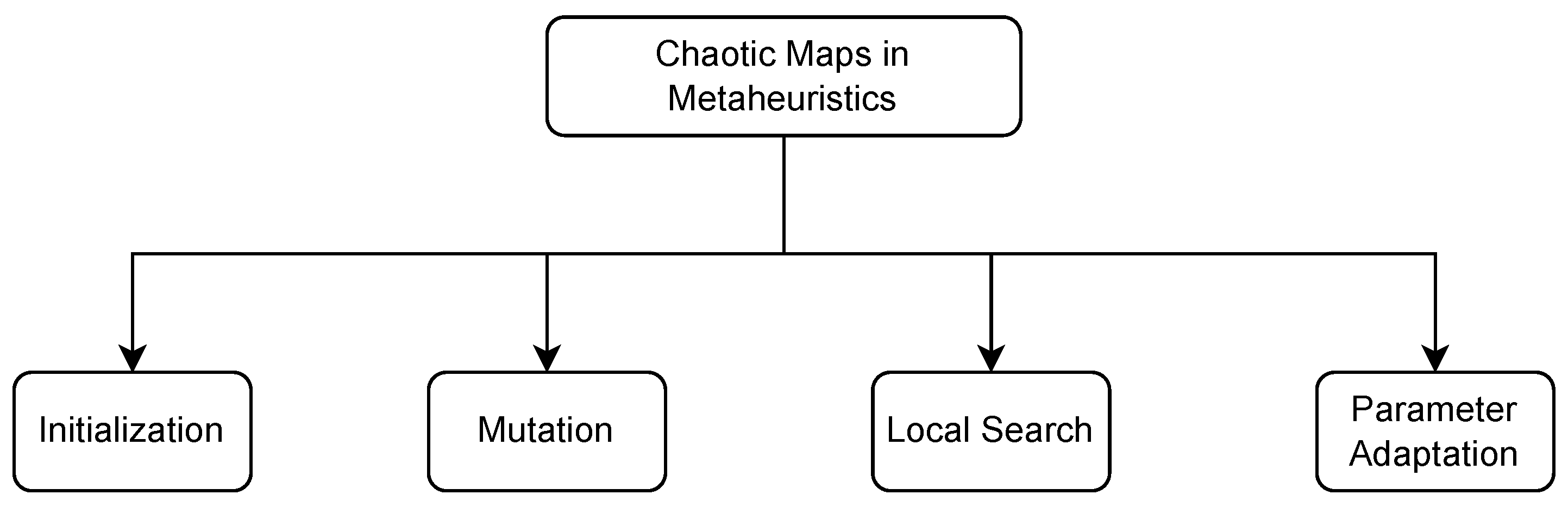
2.3. Chaotic Maps in Metaheuristics

Hybridization between metaheuristics and chaotic maps can be classified into four categories, which are summarized in Figure 2.

Initialization: The implementation of chaotic maps can be effective in creating initial solutions or populations in metaheuristic techniques, thereby replacing the random generation of these solutions. The nature of chaotic dynamics facilitates the distribution of initial solutions in different areas of the search space, thereby enhancing the exploration phase [13,17,18,55,56,57,58,59].
Mutation: Chaotic maps can be employed to perturb or mutate solutions. By using the chaotic behavior as a source of randomness, the metaheuristic algorithm can introduce diverse and unpredictable variations in the solutions, aiding in exploration [15,60,61].
Local Search: Chaotic maps have the potential to effectively steer the local search process within metaheuristic algorithms. By integrating chaotic dynamics into the metaheuristics, the algorithm gains the ability to break free from local optima and delve into various segments of the solution space [14,50,62,63,64,65,66].
Parameter Adaptation: Chaos maps can be employed to dynamically adapt the parameters of a metaheuristic. The inherent chaotic behavior aids in the real-time adjustment of metaheuristic-specific parameters such as mutation rates and crossover probabilities in a genetic algorithm, thereby enhancing the algorithm’s adaptability throughout the optimization process [12,19,20,67,68,69,70,71,72,73].

3. Continuous Metaheuristics for Solving Combinatorial Problems

The No Free Lunch (NFL) theorem [47,48,49] indicates that there is no optimization algorithm capable of solving all existing optimization problems effectively. This is the primary motivation behind binarizing continuous metaheuristics, as evident in the literature where authors have presented binary versions for the Bat Algorithm [74,75], Particle Swarm Optimization [76], Sine Cosine Algorithm [10,11,77,78], Salp Swarm Algorithm [79,80], Grey Wolf Optimizer [11,81,82], Dragonfly Algorithm [83,84], Whale Optimization Algorithm [11,77,85], and Magnetic Optimization Algorithm [86].

The binarization process aims to transfer continuous solutions from a metaheuristic to the binary domain. In the literature [22], various binarization methods are found, with the two-step technique being a notable one. Researchers use this technique because of its quick implementation and integration into metaheuristics [87,88].

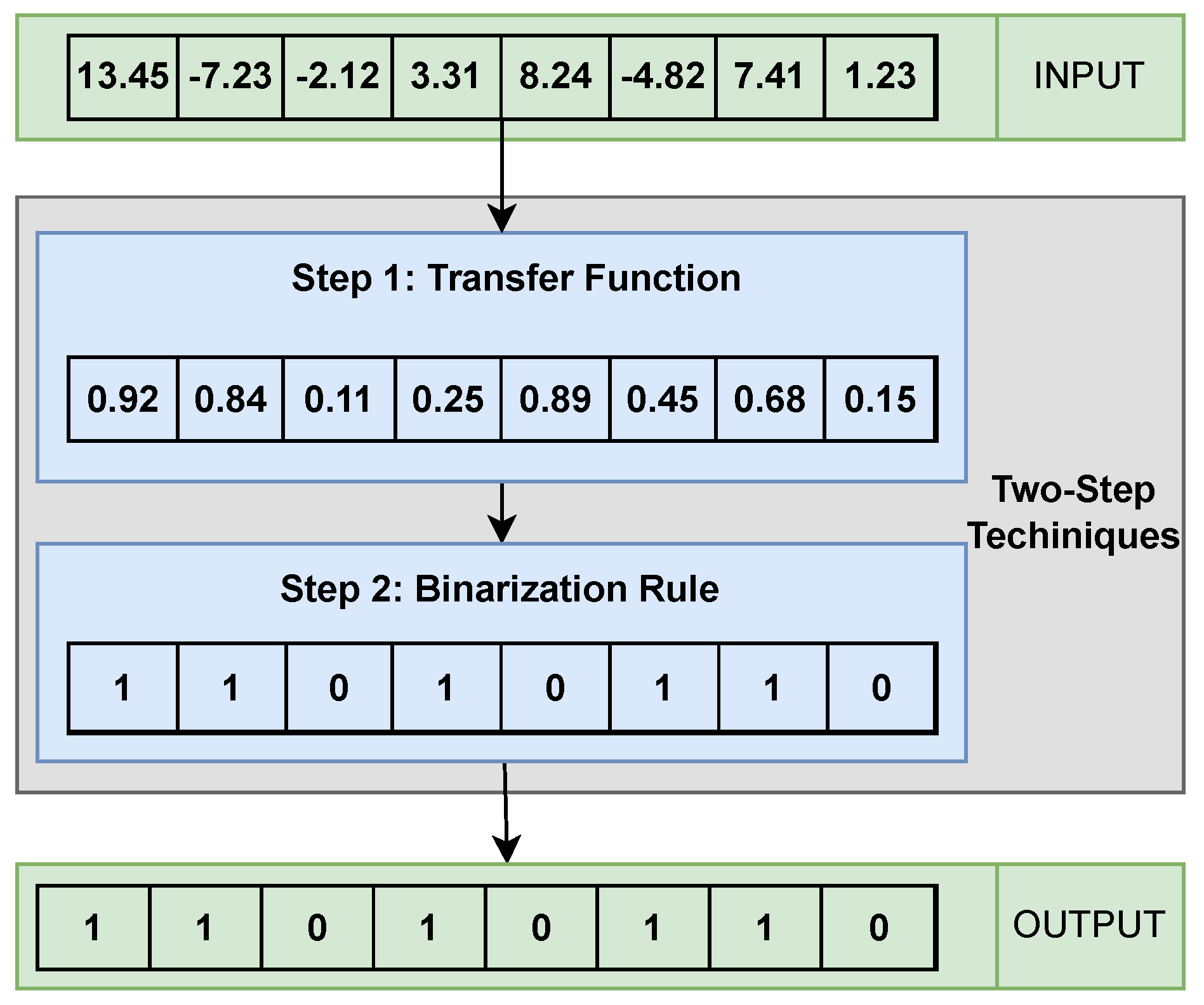
3.1. Two-Step Technique

The two-step technique, as its name suggests, performs the binarization process in two stages. In the first stage, a transfer function is applied, which maps continuous solutions to the real domain

[0, 1]

. Then, in the second stage, a binarization rule is applied, discretizing the transferred value, thereby completing the binarization process. Figure 3 provides an overview of the two-step technique.

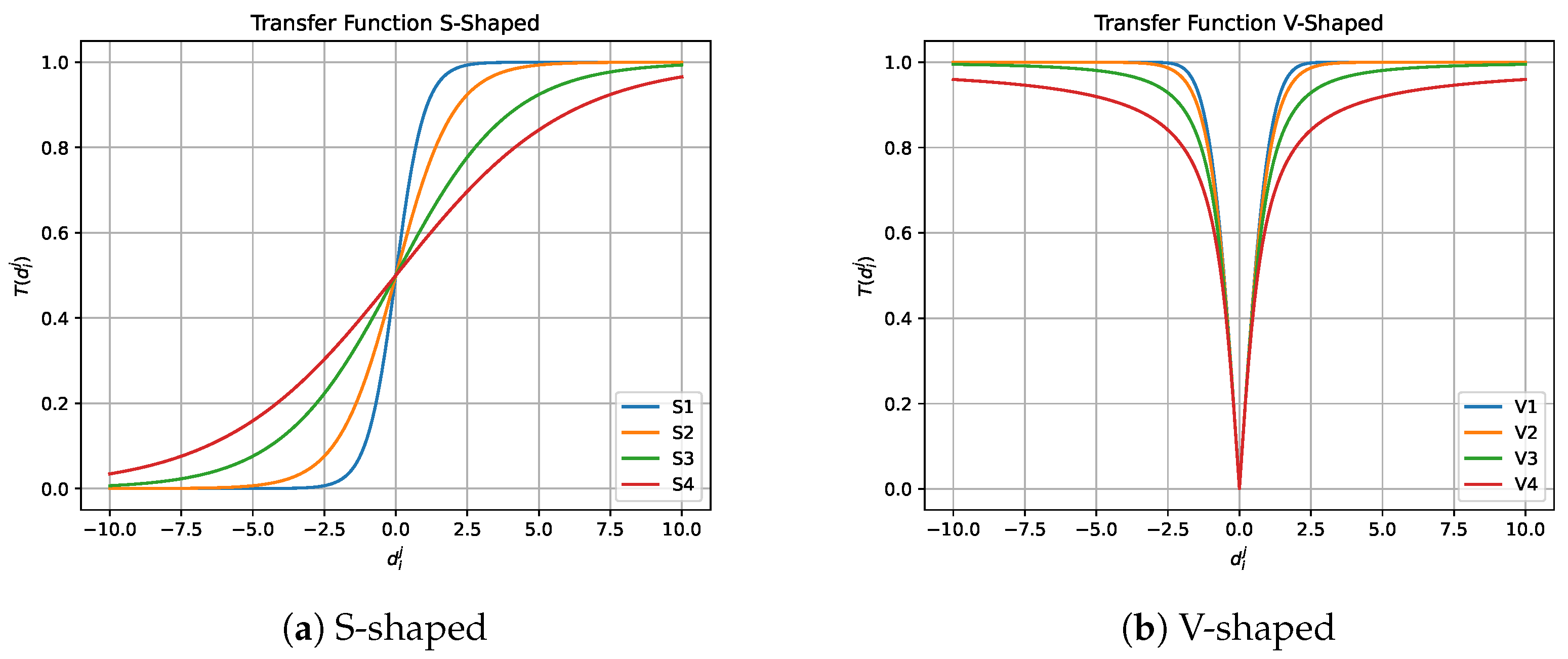
3.1.1. Transfer Function

In 1997, Kennedy et al. [89] introduced transfer functions in the field of optimization. New transfer functions have been introduced over the years [22], and we can observe that there are different types of transfer functions, among which S-Shaped transfer functions [76,90] and V-Shaped transfer functions [91] stand out.

Table 1 and Figure 4 show the S-Shaped transfer functions and V-Shaped transfer functions found in the literature. The notation

d_{i}^{j}

observed in Table 1 corresponds to the continuous value of the j-th dimension of the i-th individual resulting after the perturbation performed by the continuous metaheuristic.

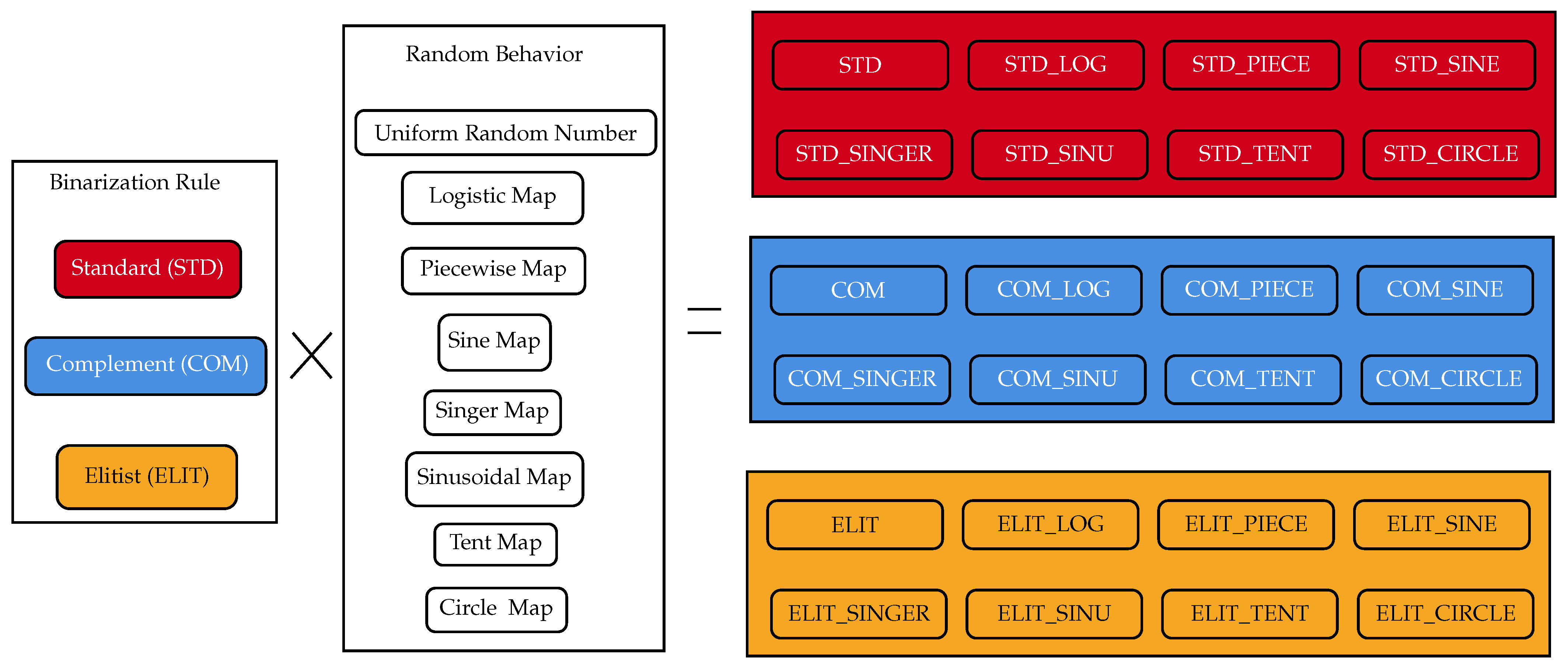
3.1.2. Binarization Rule

The process of binarization involves converting continuous values into binary values, that is, values of 0 or 1. In this context, binarization rules are applied to the probability obtained from the transfer function to obtain a binary value. There are various different rules described in scientific literature [92] that can be utilized for this binarization process. The choice of the binarization rule is crucial since it can vary depending on the context and specific problem needs. It is crucial to consider the appropriate use of the binarization rule to obtain accurate and reliable results. Table 2 shows the five binarization rules found in the literature [87].

The notation

X_{i}^{j}

observed in Table 2 corresponds to the j-th dimension binary value of the i-th current individual, and

X_{B e s t}^{j}

, observed also in Table 2, corresponds to the j-th dimension binary value of the best solution. Algorithm 4 shows the general scheme of a continuous metaheuristic being binarized. The

Δ

symbol observed there refers to the perturbation of solutions, which is implemented by each metaheuristic in its own way depending on its inspiration.

Algorithm 4 General scheme of continuous MHs for solving combinatorial problems

Input: The population

X = {X_{1}, X_{2}, \dots, X_{p o p}}

Output: The updated population

X^{'} =

{X_{1}^{'}, X_{2}^{'}, \dots, X_{p o p}^{'}}

and

X_{b e s t}

1:: Initialize random binary population X
2:: for $t = 1$ to $M a x_{i t e r}$ do
3:: for $i = 1$ to $p o p$ do
4:: for $j = 1$ to $d i m$ do
5:: $X_{i, j}^{t + 1} = X_{i, j}^{t} + Δ$
6:: end for
7:: end for
8:: for $i = 1$ to $p o p$ do ▹ Binarization Process
9:: for $j = 1$ to $d i m$ do
10:: Get $T (d_{i}^{j})$ by applying transfer function
11:: Get $X_{n e w}^{j}$ by applying binarization rule
12:: end for
13:: end for
14:: Evaluate each solution on the objective function
15:: Update $X_{b e s t}$
16:: end for

4. Proposal: Chaotic Binarization Schemes

Authors who have incorporated chaotic behavior into their metaheuristics indicate that they improve the balance of exploration and exploitation because they obtain better results. On the other hand, Senkerik in [93] shows us a study on chaos dynamics in metaheuristics and tells us the choice of chaotic maps depends closely on the problem to be solved.

As observed in Section 2.3, chaotic maps have been applied to replace the random numbers used in metaheuristics. In this context, we propose using chaotic behavior to carry out the binarization process.

Specifically, we propose replacing the random numbers used in the standard binarization rule, complement binarization rule, and elitist binarization rule with the chaotic numbers generated by the chaotic maps.

As shown in Section 2.2, there are different chaotic maps; some of them can encourage exploration, and others can encourage exploitation. Thus, each original binarization rule will be compared with seven new chaotic variants for each binarization rule; these are detailed in Figure 5.

In other words, our proposal consists of changing the uniform distribution between [0, 1] of the random number existing in the standard binarization rule, complementary binarization rule, and elitist binarization rule by the chaotic distribution of the 7 chaotic maps defined in the present work.

The dimensionality of the chaotic maps will be related to the number of iterations (

M a x_{i t e r}

), population size (

p o p

), and number of decision variables of the optimization problem (

d i m

). Thus, the dimensionality of the chaotic maps in the present proposal will be

M a x_{i t e r} \cdot p o p \cdot d i m

. Suppose we have an optimization problem with 100 decision variables and we use a population of 10 individuals and 500 iterations. In this case, the generated chaotic map will contain

100 \cdot 10 \cdot 500

values. Algorithm 5 presents a summary of the proposal.

Algorithm 5 Chaotic binarization schemes

Input: The population

X = {X_{1}, X_{2}, \dots, X_{p o p}}

Output: The updated population

X^{'} =

{X_{1}^{'}, X_{2}^{'}, \dots, X_{p o p}^{'}}

and

X_{b e s t}

1:: Initialize random binary population X
2:: Initialize the chaotic maps using $M a x_{i t e r}$ , $p o p$ and $d i m$
3:: for $t = 1$ to $M a x_{i t e r}$ do
4:: for $i = 1$ to $p o p$ do
5:: for $j = 1$ to $d i m$ do
6:: $X_{i, j}^{t + 1} = X_{i, j}^{t} + Δ$
7:: end for
8:: end for
9:: for $i = 1$ to $p o p$ do ▹ Binarization Process
10:: for $j = 1$ to $d i m$ do
11:: Get $T (d_{i}^{j})$ by applying transfer function
12:: Get chaotic map value
13:: Get $X_{n e w}^{j}$ by applying binarization rule using chaotic number
14:: end for
15:: end for
16:: Evaluate each solution on the objective function
17:: Update $X_{b e s t}$
18:: end for

5. Experimental Results

To validate our proposal we used the Grey Wolf Optimizer, Sine Cosine Algorithm, and Whale Optimization Algorithm. Each of these continuous metaheuristics was used to solve a set of benchmark instances of the 0-1 Knapsack Problem. The binarization process of each of these metaheuristics is shown in Figure 5. We have 24 different versions of each metaheuristic. To test our proposal, we use benchmark instances widely used in the literature.

5.1. 0-1 Knapsack Problem

The Knapsack Problem is another NP-hard combinatorial optimization problem. Mathematically, it is modeled as follows: Given N objects, where the j-th object has its own weight

w_{j}

and profit

p_{j}

, and a knapsack that can holds a limited weight capability C, the problem consists of finding the objects that maximize the profit whose sum of weights does not exceed the capacity of the knapsack [94,95,96]. The objective function is as follows:

max f (x) = \sum_{j = 1}^{N} p_{j} x_{j}

(8)

This is subject to the following restrictions:

\begin{matrix} \sum_{j = 1}^{N} w_{j} x_{j} \leq C \\ x_{j} \in {0, 1} \forall j \in J \end{matrix}

(9)

where

x_{j}

represents the binary decision variables (i.e., whether an element is considered in the knapsack (value 1 in the decision variable) or not considered in the knapsack (value 0 in the decision variable)).

According to the authors in [97], this problem has different practical applications in the real world, such as capital budgeting allocation problems [98], resource allocation problems [99], stock-cutting problems [100], and investment decision making [101].

We use the instances proposed by Pisinger in [102,103] where he presents three sets of benchmark instances that differ due to the correlation between each element. Table 3 shows the details of the benchmark instances of the Knapsack Problem used in this work, where the first column of this table presents the name of the instance, the second column presents the number of items to select, and the third column presents the global optimum of the instance.

5.2. Parameter Setting

Regarding the setup of the experiments, each variation of the metaheuristics was run 31 times independently, a population size of 20 individuals was used, and 500 iterations were used. The details of each configuration are detailed in Table 4.

Thus,

3 \times 31 \times 15 \times 24 = 33, 480

experiments were carried out. Regarding the software and hardware used in the experimentation, we used Python in version 3.10.5 64-bit as the programming language. All the experiments were executed on a machine with Windows 10, an Intel Core i9-10900k 3.70 GHz processor, and 64 GB of RAM.

5.3. Summary of Results

Table 5 shows us the performance of each experiment with the three metaheuristics used in each solved instance. The first column of the table indicates the experiment, while the second and third columns pertain to the solved instance. The second column shows two symbols. The symbol “✓” indicates that the experiment under analysis reached the known global optimum, while the symbol “×” indicates that the experiment under analysis did not reach the known global optimum. Finally, in the third column we will also observe two things. In case the experiment under analysis has reached the known global optimum, this column will indicate in bold and underlined the metaheuristic(s) that reached the global optimum. In case no metaheuristic has reached the optimum, the metaheuristic or metaheuristics that reached the value closest to the optimum will be reported without bold and underlined. This last case applies to instances knapPI_2_100_1000_1, knapPI_2_1000_1000_1, knapPI_1_2000_1000_1, knapPI_2_2000_1000_1, and knapPI_3_2000_1000_1.

By analyzing Table 5 we can observe that the experiments incorporating the standard binarization rule and the complement binarization rule have the best results. In particular, we can highlight the family of experiments incorporating the standard binarization rule since they reach the optimum in instances knapPI_1_500_1000_1, knapPI_2_500_1000_1, knapPI_3_500_1000_1, knapPI_1_1000_1000_1, and knapPI_3_1000_1000_1.

Table 6, Table 7 and Table 8 show the results obtained using GWO, WOA, and SCA, respectively. In these tables, we observe the following: in the first column, we observe the experiment used as defined in Figure 5, and the second, third, and fourth columns are repeated for each solved instance. The first of them indicates the best result obtained, the second of them indicates the average obtained with the 31 runs performed, and the third of them indicates the Relative Percentage Distance (RPD), which is calculated based on Equation (10). The experiments are grouped by base binarization rule, and the best result obtained per family is highlighted in bold and underlined.

RPD = \frac{100 \cdot (O p t - B e s t)}{O p t} .

(10)

where

O p t

corresponds to the optimum of the instance and

B e s t

corresponds to the best value obtained for the experiment.

When analyzing the results obtained in Table 6, Table 7 and Table 8, we can observe that the best binarization rule is STD_TENT, which reached the optimum with the three metaheuristics in 8 instances out of the 15 solved, and with WOA the optimum was reached in 2 more instances. In addition, with WOA the best result was reached in 1 instance.

This confirms what the authors have previously pointed out: the incorporation of chaotic maps improves performance in metaheuristics.

On the other hand, when we look at the largest instances (i.e., instances knapPI_1_1000_ 1000_1, knapPI_2_1000_1000_1, knapPI_3_1000_1000_1, knapPI_1_2000_1000_1, knapPI_2_ 2000_1000_1, and knapPI_3_2000_1000_1), we can observe that the WOA with the standard binarization rule achieves the best results, reaching the optimum in one and two. This indicates that the perturbation operators used by WOA to move the solutions in the search space are more efficient than the SCA and GWO operators.

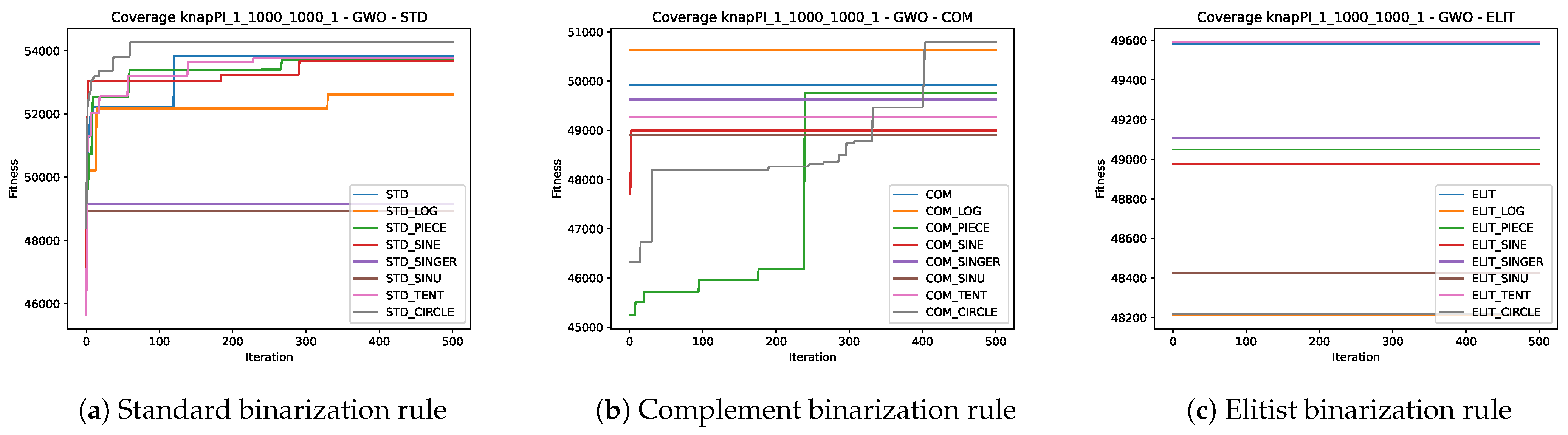
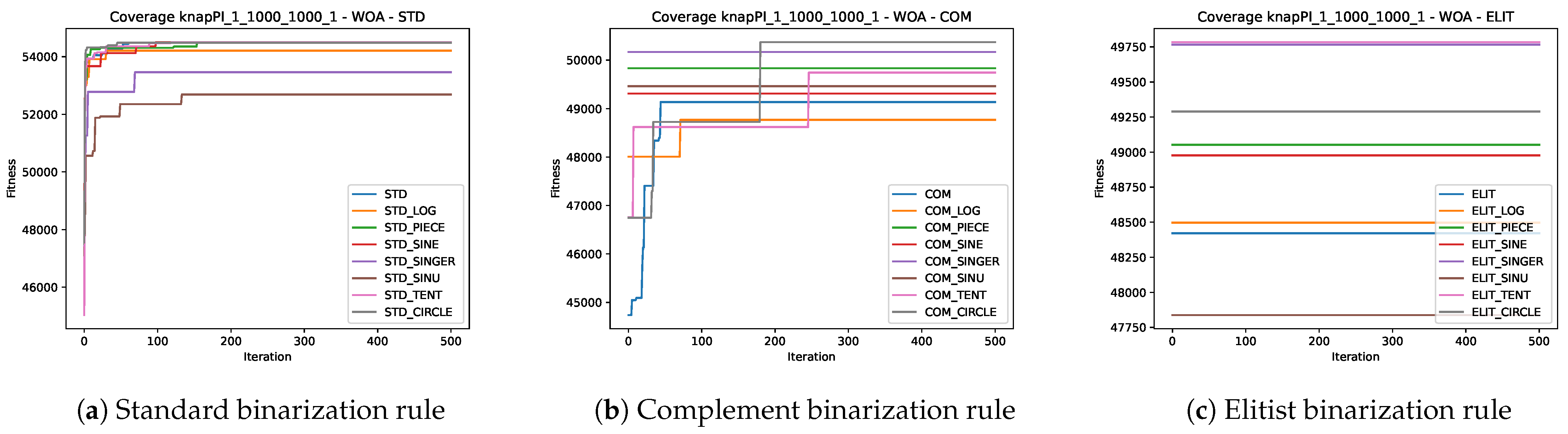
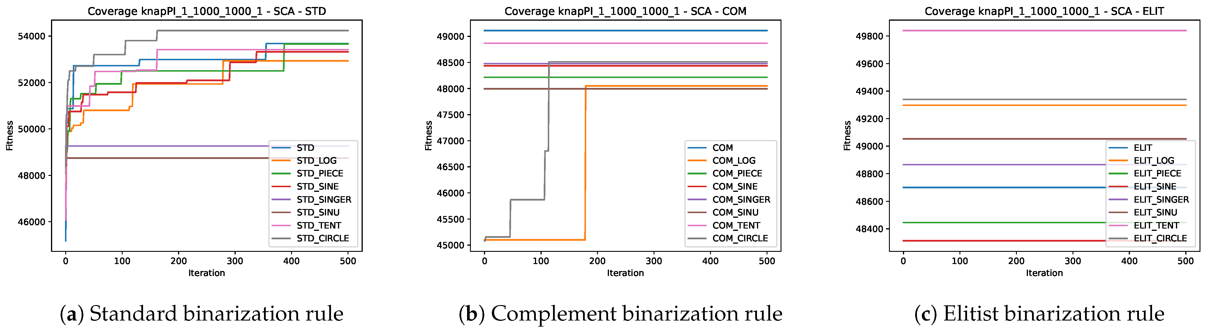
5.4. Convergence Analysis

In this section, the convergence speed of the 24 experiments associated with the three metaheuristics will be analyzed by solving the knapPI_1_1000_1000_1 instance. This instance was selected since all the algorithms have similar behaviors in all instances, so the choice was random. For more information, you can consult the GitHub repository associated with this paper so you can see the behavior in the other instances.

Figure 6a, Figure 7a, and Figure 8a show us the behavior of the experiments that include the standard binarization rule in GWO, WOA, and SCA, respectively. In all three metaheuristics, we can observe that the STD_SINGER and STD_SINU experiments exhibit premature stagnation, unlike the others, which demonstrate decent convergence.

On the other hand, in Figure 6b, Figure 7b, and Figure 8b, the behavior of the experiments that include the complement binarization rule in GWO, WOA, and SCA is observed respectively. An unusual behavior is observed where several experiments fail to improve the initial optimum generated by the initial solutions. Furthermore, this behavior is not uniform across the three metaheuristics. For GWO, the experiments COM_PIECE and COM_CIRCLE converge, while for WOA, it is COM, COM_CIRCLE, and COM_TENT, and for SCA, it is COM_TENT and COM_CIRCLE.

Finally, Figure 6c, Figure 7c, and Figure 8c show us the behavior of the experiments that include the elitist binarization rule in GWO, WOA, and SCA, respectively. In this case, it is even more noticeable since all experiments for the three metaheuristics do not improve upon the initial solutions obtained with the generation of initial solutions. This is striking and suggests that when using the elitist binarization rule, the solutions become lost in the search space.

Here again, we can observe two important things. The first is that the binarization rule plays a significant role, and the second is that chaotic maps do have an impact on convergence.

On the other hand, observing the behavior of the experiments that use as a basis the standard binarization rule and complement binarization rule within WOA, we can observe that it has a premature convergence and good results, unlike SCA and GWO, which have a slower convergence. This confirms what we mentioned in Section 5.3: the perturbation operators of WOA solutions are more efficient in exploring and exploiting the search space.

5.5. Statistical Test

In the literature [9,104,105,106], it can be seen that the authors perform a static test to compare the experimental results to determine if there is any significant difference between each experiment. For this type of experimentation, a non-parametric statistical test must be applied. In response to this, we have applied the Wilcoxon–Mann–Whitney test [107,108].

From the Scipy Python library, we can apply this statistical test. The python function is called scipy.stats.mannwhitneyu. One parameter of the above function is “alternative”, which we define as “greater”. We evaluate and contrast two distinct experiments, as previously stated in Figure 5. Thus, we can state the following hypotheses:

H_{0} = E x p e r i m e n t A \leq E x p e r i m e n t B

H_{1} = E x p e r i m e n t A > E x p e r i m e n t B

If the result of the statistical test is with obtained a p-value < 0.05, we cannot assume that

E x p e r i m e n t

B has worse performance than

E x p e r i m e n t

A, rejecting

H_{0}

. This comparison is made because our problem is a maximization problem.

Table 9 shows a summary of the statistical comparisons made. The first column indicates the 24 experiments, the second column indicates how many times the experiment was better than another when we used GWO, the third column indicates how many times the experiment was better than another when we used WOA, the fourth column tells us how many times the experiment was better than the other when we used SCA, and the fifth column tells us how many times one experiment was better than the other when we consider the three metaheuristics. In such a case, metaheuristics compare one experiment against 23 others.

By analyzing Table 9, we can see that the experiments that include the elitist binarization rule are the best in the three metaheuristics. If we check carefully, we can see that ELIT_CIRCLE is statistically worse than the rest of the experiments that include the binarization rule except when we compare with SCA, where only ELIT and ELIT_LOG are statistically better than ELIT_CIRCLE.

After observing all the experiments of the elitist binarization rule family, we can observe the experiments COM_SINU, composed of the complement binarization rule and the capotic sinusoidal map, and STD_SINU, composed of the standard binarization rule and the chaotic sinusoidal map. This is interesting since we can see that the incorporation of the chaotic sinusoidal map contributed to obtaining better results. Although they do not reach optimality in each instance, they are statistically better than the other experiments that include the complement and standard binarization rules.

Another interesting point is that the family of experiments composed by the complement binarization rule obtains statistically better results than those composed of the standard binarization rule with the three metaheuristics used. Finally, the worst experiments are those that include the standard binarization rule, except STD_SINU, since statistically, they fail to beat any other experiment.

Given the experimental results and the statistical tests applied, we can indicate that the binarization rule has a high impact on the binarization process of continuous metaheuristics, as indicated by the authors in [104]. In addition to this, chaotic maps also have an impact on the behavior of metaheuristics, which can be observed in the experimental results, convergence graphs, and statistical tests.

Table 10 shows the results when comparing the 24 experiments applied in GWO, Table 11 shows the results when comparing the 24 experiments applied in WOA, and Table 12 show the results when 24 experiments applied in WOA. These tables are structured as follows: the first column presents the techniques used (Experiment A), and the following columns present the average p-values of the seven instances compared with the version indicated in the column title (Experiment B). The values highlighted in bold and underlined show when the statistical test gives us a value less than 0.05, which is when the null hypothesis (

H_{0}

) is rejected. Additionally, when we compare the same experiment, it is marked with an “X” symbol.

6. Conclusions

Binary combinatorial problems, such as the Set Covering Problem [9,11,77,104,105], Knapsack Problem [109,110], or Cell Formation Problem [106], are increasingly common in the industry. Given the demand for good results in reasonable times, metaheuristics have begun to gain ground as resolution techniques.

In the literature [21], we can find different continuous metaheuristics, most of which are designed to solve continuous optimization problems. In view of this, it is necessary to apply a binarization process so that they can solve binary combinatorial problems.

Among the best-known binarization processes [22] found is the two-step technique, which uses a transfer function and the binarization rule [87]. Among the binarization rules are the standard binarization rule, the complement binarization rule, and the elitist binarization rule. These three have one factor in common, and that is that they use a random number within the rules.

Our proposal consists of changing the behavior of the random number of the three binarization rules mentioned above by replacing it with chaotic maps. In particular, we use seven different chaotic maps within the three binarization rules mentioned above, thus creating eight experiments, where seven of them use the chaotic maps and the remaining is the original version that uses a random number with a uniform distribution. Regarding the experiments, seven instances and three metaheuristics were widely solved in the literature.

In the present work, it was shown that the incorporation of chaotic maps has a great impact on the behavior of the three metaheuristics considered. This is interesting since it confirms what has been said in the literature, that chaotic maps impact exploration and exploitation and, consequently, obtain better results.

Of all the experiments carried out, we can highlight all those that are based on the standard binarization rule and complement binarization rule since they are statistically better in the three metaheuristics compared to the experiment that is based on the elitist binarization rule.

Given this, we propose a strategy to select the best binarization rule and chaotic map. First, experiment with some instances of the problem using the three binarization rules without modification (i.e., use the standard, complement, and elitist binarization rules) to see which rule is the most suitable. Once the rule is chosen, proceed to experiment with the incorporation of chaotic maps to show which one has more impact during the optimization process. This strategy can be used independently of the binary combinatorial optimization problem to be solved.

As future work, we propose to use this approach in other binary combinatorial optimization problems, such as the Feature Selection Problem or Set Covering Problem, as well as to incorporate these chaotic maps in other binarization rules, such as elitist roulette.

Furthermore, in the literature, there are proposals that use machine learning techniques from the reinforcement learning family to dynamically select binarization schemes during the optimization process [9,10,11,81,85,111]. This work can be extended to use these new binarization schemes as actions to be decided by machine learning techniques to dynamically balance exploration and exploitation.

Author Contributions

Conceptualization, F.C.-C. and B.C.; methodology, F.C.-C. and B.C.; software, F.C.-C.; validation, B.C., R.S., G.G., Á.P. and A.P.F.; formal analysis, F.C.-C.; investigation, F.C.-C., B.C., R.S., G.G., Á.P. and A.P.F.; resources, F.C.-C.; writing—original draft F.C.-C. and B.C.; writing—review and editing, R.S., G.G., Á.P. and A.P.F.; supervision, B.C. and R.S.; funding acquisition, B.C. and R.S. All authors have read and agreed to the published version of the manuscript.

Funding

This research received no external funding.

Data Availability Statement

All the results of this work are available at the GitHub repository (https://github.com/FelipeCisternasCaneo/Chaotic-Binarization-Schemes-for-Solving-Combinatorial-Optimization-Problems.git (accessed on 1 January 2024)) and the database with results (https://drive.google.com/drive/folders/1MpSG6qlQ8d8k-qpalebzJFzbJ-DhFObb?usp=sharing (accessed on 1 January 2024)). GitHub has a limit of 100 MB for a file uploaded to the repository. This is why we have left the database shared on Google Drive. To perform validations, you only need to download the file in the shared Google Drive folder, clone the repository, and incorporate the downloaded file in the “BD” folder of the cloned repository.

Acknowledgments

Broderick Crawford and Ricardo Soto are supported by the grant ANID/FONDECYT/REGULAR/1210810. Felipe Cisternas-Caneo is supported by the National Agency for Research and Development (ANID)/Scholarship Program/DOCTORADO NACIONAL/2023-21230203. Felipe Cisternas-Caneo, Broderick Crawford, Ricardo Soto, Álex Paz, and Alvaro Peña Fritz are supported by grant DI Centenario/VINCI/PUCV/039.368/2023.

Conflicts of Interest

The authors declare no conflicts of interest.

References

Talbi, E.G. Metaheuristics: From Design to Implementation; John Wiley & Sons: Hoboken, NJ, USA, 2009. [Google Scholar]
Abdel-Basset, M.; Sallam, K.M.; Mohamed, R.; Elgendi, I.; Munasinghe, K.; Elkomy, O.M. An Improved Binary Grey-Wolf Optimizer With Simulated Annealing for Feature Selection. IEEE Access 2021, 9, 139792–139822. [Google Scholar] [CrossRef]
Zhao, M.; Hou, R.; Li, H.; Ren, M. A hybrid grey wolf optimizer using opposition-based learning, sine cosine algorithm and reinforcement learning for reliable scheduling and resource allocation. J. Syst. Softw. 2023, 205, 111801. [Google Scholar] [CrossRef]
Ahmed, K.; Salah Kamel, F.J.; Youssef, A.R. Hybrid Whale Optimization Algorithm and Grey Wolf Optimizer Algorithm for Optimal Coordination of Direction Overcurrent Relays. Electr. Power Components Syst. 2019, 47, 644–658. [Google Scholar] [CrossRef]
Seyyedabbasi, A. WOASCALF: A new hybrid whale optimization algorithm based on sine cosine algorithm and levy flight to solve global optimization problems. Adv. Eng. Softw. 2022, 173, 103272. [Google Scholar] [CrossRef]
Tapia, D.; Crawford, B.; Soto, R.; Cisternas-Caneo, F.; Lemus-Romani, J.; Castillo, M.; García, J.; Palma, W.; Paredes, F.; Misra, S. A Q-Learning Hyperheuristic Binarization Framework to Balance Exploration and Exploitation. In Proceedings of the International Conference on Applied Informatics, Ota, Nigeria, 29–31 October 2020; Florez, H., Misra, S., Eds.; Springer International Publishing: Cham, Switzerland, 2020; pp. 14–28. [Google Scholar] [CrossRef]
De Oliveira, S.G.; Silva, L.M. Evolving reordering algorithms using an ant colony hyperheuristic approach for accelerating the convergence of the ICCG method. Eng. Comput. 2020, 36, 1857–1873. [Google Scholar] [CrossRef]
Gonzaga de Oliveira, S.; Silva, L. An ant colony hyperheuristic approach for matrix bandwidth reduction. Appl. Soft Comput. 2020, 94, 106434. [Google Scholar] [CrossRef]
Becerra-Rozas, M.; Lemus-Romani, J.; Cisternas-Caneo, F.; Crawford, B.; Soto, R.; García, J. Swarm-Inspired Computing to Solve Binary Optimization Problems: A Backward Q-Learning Binarization Scheme Selector. Mathematics 2022, 10, 4776. [Google Scholar] [CrossRef]
Cisternas-Caneo, F.; Crawford, B.; Soto, R.; de la Fuente-Mella, H.; Tapia, D.; Lemus-Romani, J.; Castillo, M.; Becerra-Rozas, M.; Paredes, F.; Misra, S. A Data-Driven Dynamic Discretization Framework to Solve Combinatorial Problems Using Continuous Metaheuristics. In Proceedings of the International Conference on Innovations in Bio-Inspired Computing and Applications, Ibica, Spain, 16–18 December 2021; Abraham, A., Sasaki, H., Rios, R., Gandhi, N., Singh, U., Ma, K., Eds.; Springer International Publishing: Cham, Switzerland, 2021; pp. 76–85. [Google Scholar] [CrossRef]
Lemus-Romani, J.; Becerra-Rozas, M.; Crawford, B.; Soto, R.; Cisternas-Caneo, F.; Vega, E.; Castillo, M.; Tapia, D.; Astorga, G.; Palma, W.; et al. A Novel Learning-Based Binarization Scheme Selector for Swarm Algorithms Solving Combinatorial Problems. Mathematics 2021, 9, 2887. [Google Scholar] [CrossRef]
Ibrahim, A.M.; Tawhid, M.A. Chaotic electromagnetic field optimization. Artif. Intell. Rev. 2022, 56, 9989–10030. [Google Scholar] [CrossRef]
Chou, J.S.; Truong, D.N. Multiobjective forensic-based investigation algorithm for solving structural design problems. Autom. Constr. 2022, 134, 104084. [Google Scholar] [CrossRef]
Gao, S.; Yu, Y.; Wang, Y.; Wang, J.; Cheng, J.; Zhou, M. Chaotic Local Search-Based Differential Evolution Algorithms for Optimization. IEEE Trans. Syst. Man, Cybern. Syst. 2021, 51, 3954–3967. [Google Scholar] [CrossRef]
Agrawal, P.; Ganesh, T.; Mohamed, A.W. Chaotic gaining sharing knowledge-based optimization algorithm: An improved metaheuristic algorithm for feature selection. Soft Comput. 2021, 25, 9505–9528. [Google Scholar] [CrossRef]
Naanaa, A. Fast chaotic optimization algorithm based on spatiotemporal maps for global optimization. Appl. Math. Comput. 2015, 269, 402–411. [Google Scholar] [CrossRef]
Yang, H.; Yu, Y.; Cheng, J.; Lei, Z.; Cai, Z.; Zhang, Z.; Gao, S. An intelligent metaphor-free spatial information sampling algorithm for balancing exploitation and exploration. Knowl.-Based Syst. 2022, 250, 109081. [Google Scholar] [CrossRef]
Khosravi, H.; Amiri, B.; Yazdanjue, N.; Babaiyan, V. An improved group teaching optimization algorithm based on local search and chaotic map for feature selection in high-dimensional data. Expert Syst. Appl. 2022, 204, 117493. [Google Scholar] [CrossRef]
Mohmmadzadeh, H.; Gharehchopogh, F.S. An efficient binary chaotic symbiotic organisms search algorithm approaches for feature selection problems. J. Supercomput. 2021, 77, 9102–9144. [Google Scholar] [CrossRef]
Pichai, S.; Sunat, K.; Chiewchanwattana, S. An asymmetric chaotic competitive swarm optimization algorithm for feature selection in high-dimensional data. Symmetry 2020, 12, 1782. [Google Scholar] [CrossRef]
Rajwar, K.; Deep, K.; Das, S. An exhaustive review of the metaheuristic algorithms for search and optimization: Taxonomy, applications, and open challenges. Artif. Intell. Rev. 2023, 56, 13187–13257. [Google Scholar] [CrossRef]
Becerra-Rozas, M.; Lemus-Romani, J.; Cisternas-Caneo, F.; Crawford, B.; Soto, R.; Astorga, G.; Castro, C.; García, J. Continuous Metaheuristics for Binary Optimization Problems: An Updated Systematic Literature Review. Mathematics 2022, 11, 129. [Google Scholar] [CrossRef]
Mirjalili, S. SCA: A sine cosine algorithm for solving optimization problems. Knowl.-Based Syst. 2016, 96, 120–133. [Google Scholar] [CrossRef]
Mirjalili, S.; Mirjalili, S.M.; Lewis, A. Grey wolf optimizer. Adv. Eng. Softw. 2014, 69, 46–61. [Google Scholar] [CrossRef]
Mirjalili, S.; Lewis, A. The whale optimization algorithm. Adv. Eng. Softw. 2016, 95, 51–67. [Google Scholar] [CrossRef]
Banerjee, A.; Nabi, M. Re-entry trajectory optimization for space shuttle using sine-cosine algorithm. In Proceedings of the 2017 8th International Conference on Recent Advances in Space Technologies (RAST), Istanbul, Turkey, 19–22 June 2017; pp. 73–77. [Google Scholar] [CrossRef]
Sindhu, R.; Ngadiran, R.; Yacob, Y.M.; Zahri, N.A.H.; Hariharan, M. Sine–cosine algorithm for feature selection with elitism strategy and new updating mechanism. Neural Comput. Appl. 2017, 28, 2947–2958. [Google Scholar] [CrossRef]
Mahdad, B.; Srairi, K. A new interactive sine cosine algorithm for loading margin stability improvement under contingency. Electr. Eng. 2018, 100, 913–933. [Google Scholar] [CrossRef]
Padmanaban, S.; Priyadarshi, N.; Holm-Nielsen, J.B.; Bhaskar, M.S.; Azam, F.; Sharma, A.K.; Hossain, E. A novel modified sine-cosine optimized MPPT algorithm for grid integrated PV system under real operating conditions. IEEE Access 2019, 7, 10467–10477. [Google Scholar] [CrossRef]
Gonidakis, D.; Vlachos, A. A new sine cosine algorithm for economic and emission dispatch problems with price penalty factors. J. Inf. Optim. Sci. 2019, 40, 679–697. [Google Scholar] [CrossRef]
Abd Elfattah, M.; Abuelenin, S.; Hassanien, A.E.; Pan, J.S. Handwritten arabic manuscript image binarization using sine cosine optimization algorithm. In Proceedings of the International Conference on Genetic and Evolutionary Computing, Fuzhou, China, 7–9 November 2016; pp. 273–280. [Google Scholar] [CrossRef]
Emary, E.; Zawbaa, H.M.; Grosan, C.; Hassenian, A.E. Feature subset selection approach by gray-wolf optimization. In Proceedings of the Afro-European Conference for Industrial Advancement, Villejuif, France, 9–11 September 2015; pp. 1–13. [Google Scholar] [CrossRef]
Kumar, V.; Chhabra, J.K.; Kumar, D. Grey wolf algorithm-based clustering technique. J. Intell. Syst. 2017, 26, 153–168. [Google Scholar] [CrossRef]
Eswaramoorthy, S.; Sivakumaran, N.; Sekaran, S. Grey wolf optimization based parameter selection for support vector machines. COMPEL Int. J. Comput. Math. Electr. Electron. Eng. 2016, 35, 1513–1523. [Google Scholar] [CrossRef]
Li, S.X.; Wang, J.S. Dynamic modeling of steam condenser and design of PI controller based on grey wolf optimizer. Math. Probl. Eng. 2015, 2015, 120975. [Google Scholar] [CrossRef]
Wong, L.I.; Sulaiman, M.; Mohamed, M.; Hong, M.S. Grey Wolf Optimizer for solving economic dispatch problems. In Proceedings of the 2014 IEEE International Conference on Power and Energy (PECon), Kuching Sarawak, Malaysia, 1–3 December 2014; pp. 150–154. [Google Scholar] [CrossRef]
Tsai, P.W.; Nguyen, T.T.; Dao, T.K. Robot path planning optimization based on multiobjective grey wolf optimizer. In Proceedings of the International Conference on Genetic and Evolutionary Computing, Fuzhou, China, 7–9 November 2016; pp. 166–173. [Google Scholar] [CrossRef]
Lu, C.; Gao, L.; Li, X.; Xiao, S. A hybrid multi-objective grey wolf optimizer for dynamic scheduling in a real-world welding industry. Eng. Appl. Artif. Intell. 2017, 57, 61–79. [Google Scholar] [CrossRef]
Mosavi, M.R.; Khishe, M.; Ghamgosar, A. Classification of sonar data set using neural network trained by gray wolf optimization. Neural Netw. World 2016, 26, 393. [Google Scholar] [CrossRef]
Bentouati, B.; Chaib, L.; Chettih, S. A hybrid whale algorithm and pattern search technique for optimal power flow problem. In Proceedings of the 2016 8th International Conference on Modelling, Identification and Control (ICMIC), Algiers, Algeria, 15–17 November 2016; pp. 1048–1053. [Google Scholar] [CrossRef]
Touma, H.J. Study of the economic dispatch problem on IEEE 30-bus system using whale optimization algorithm. Int. J. Eng. Technol. Sci. 2016, 3, 11–18. [Google Scholar] [CrossRef]
Yin, X.; Cheng, L.; Wang, X.; Lu, J.; Qin, H. Optimization for hydro-photovoltaic-wind power generation system based on modified version of multi-objective whale optimization algorithm. Energy Procedia 2019, 158, 6208–6216. [Google Scholar] [CrossRef]
Abd El Aziz, M.; Ewees, A.A.; Hassanien, A.E. Whale optimization algorithm and moth-flame optimization for multilevel thresholding image segmentation. Expert Syst. Appl. 2017, 83, 242–256. [Google Scholar] [CrossRef]
Mafarja, M.M.; Mirjalili, S. Hybrid whale optimization algorithm with simulated annealing for feature selection. Neurocomputing 2017, 260, 302–312. [Google Scholar] [CrossRef]
Tharwat, A.; Moemen, Y.S.; Hassanien, A.E. Classification of toxicity effects of biotransformed hepatic drugs using whale optimized support vector machines. J. Biomed. Inform. 2017, 68, 132–149. [Google Scholar] [CrossRef]
Zhao, H.; Guo, S.; Zhao, H. Energy-related CO2 emissions forecasting using an improved LSSVM model optimized by whale optimization algorithm. Energies 2017, 10, 874. [Google Scholar] [CrossRef]
Igel, C. No Free Lunch Theorems: Limitations and Perspectives of Metaheuristics. In Theory and Principled Methods for the Design of Metaheuristics; Borenstein, Y., Moraglio, A., Eds.; Springer: Berlin/Heidelberg, Germany, 2014; pp. 1–23. [Google Scholar] [CrossRef]
Wolpert, D.; Macready, W. No free lunch theorems for optimization. IEEE Trans. Evol. Comput. 1997, 1, 67–82. [Google Scholar] [CrossRef]
Ho, Y.C.; Pepyne, D.L. Simple explanation of the no-free-lunch theorem and its implications. J. Optim. Theory Appl. 2002, 115, 549–570. [Google Scholar] [CrossRef]
Li, X.D.; Wang, J.S.; Hao, W.K.; Zhang, M.; Wang, M. Chaotic arithmetic optimization algorithm. Appl. Intell. 2022, 52, 16718–16757. [Google Scholar] [CrossRef]
Gandomi, A.; Yang, X.S.; Talatahari, S.; Alavi, A. Firefly algorithm with chaos. Commun. Nonlinear Sci. Numer. Simul. 2013, 18, 89–98. [Google Scholar] [CrossRef]
Arora, S.; Singh, S. An improved butterfly optimization algorithm with chaos. J. Intell. Fuzzy Syst. 2017, 32, 1079–1088. [Google Scholar] [CrossRef]
Lu, H.; Wang, X.; Fei, Z.; Qiu, M. The effects of using chaotic map on improving the performance of multiobjective evolutionary algorithms. Math. Probl. Eng. 2014, 2014, 924652. [Google Scholar] [CrossRef]
Khennaoui, A.A.; Ouannas, A.; Boulaaras, S.; Pham, V.T.; Taher Azar, A. A fractional map with hidden attractors: Chaos and control. Eur. Phys. J. Spec. Top. 2020, 229, 1083–1093. [Google Scholar] [CrossRef]
Verma, M.; Sreejeth, M.; Singh, M.; Babu, T.S.; Alhelou, H.H. Chaotic Mapping Based Advanced Aquila Optimizer With Single Stage Evolutionary Algorithm. IEEE Access 2022, 10, 89153–89169. [Google Scholar] [CrossRef]
Wang, Y.; Liu, H.; Ding, G.; Tu, L. Adaptive chimp optimization algorithm with chaotic map for global numerical optimization problems. J. Supercomput. 2023, 79, 6507–6537. [Google Scholar] [CrossRef]
Elgamal, Z.; Sabri, A.Q.M.; Tubishat, M.; Tbaishat, D.; Makhadmeh, S.N.; Alomari, O.A. Improved Reptile Search Optimization Algorithm Using Chaotic Map and Simulated Annealing for Feature Selection in Medical Field. IEEE Access 2022, 10, 51428–51446. [Google Scholar] [CrossRef]
Agrawal, U.; Rohatgi, V.; Katarya, R. Normalized Mutual Information-based equilibrium optimizer with chaotic maps for wrapper-filter feature selection. Expert Syst. Appl. 2022, 207, 118107. [Google Scholar] [CrossRef]
Wang, L.; Gao, Y.; Li, J.; Wang, X. A feature selection method by using chaotic cuckoo search optimization algorithm with elitist preservation and uniform mutation for data classification. Discret. Dyn. Nat. Soc. 2021, 2021, 7796696. [Google Scholar] [CrossRef]
Mohd Yusof, N.; Muda, A.K.; Pratama, S.F.; Carbo-Dorca, R.; Abraham, A. Improving Amphetamine-type Stimulants drug classification using chaotic-based time-varying binary whale optimization algorithm. Chemom. Intell. Lab. Syst. 2022, 229, 104635. [Google Scholar] [CrossRef]
Wang, R.; Hao, K.; Chen, L.; Wang, T.; Jiang, C. A novel hybrid particle swarm optimization using adaptive strategy. Inf. Sci. 2021, 579, 231–250. [Google Scholar] [CrossRef]
Feizi-Derakhsh, M.R.; Kadhim, E.A. An Improved Binary Cuckoo Search Algorithm For Feature Selection Using Filter Method And Chaotic Map. J. Appl. Sci. Eng. 2022, 26, 897–903. [Google Scholar] [CrossRef]
Hussien, A.G.; Amin, M. A self-adaptive Harris Hawks optimization algorithm with opposition-based learning and chaotic local search strategy for global optimization and feature selection. Int. J. Mach. Learn. Cybern. 2022, 13, 309–336. [Google Scholar] [CrossRef]
Hu, J.; Heidari, A.A.; Zhang, L.; Xue, X.; Gui, W.; Chen, H.; Pan, Z. Chaotic diffusion-limited aggregation enhanced grey wolf optimizer: Insights, analysis, binarization, and feature selection. Int. J. Intell. Syst. 2022, 37, 4864–4927. [Google Scholar] [CrossRef]
Zhang, Y.; Zhang, Y.; Zhang, C.; Zhou, C. Multiobjective Harris Hawks Optimization With Associative Learning and Chaotic Local Search for Feature Selection. IEEE Access 2022, 10, 72973–72987. [Google Scholar] [CrossRef]
Zhang, X.; Xu, Y.; Yu, C.; Heidari, A.A.; Li, S.; Chen, H.; Li, C. Gaussian mutational chaotic fruit fly-built optimization and feature selection. Expert Syst. Appl. 2020, 141, 112976. [Google Scholar] [CrossRef]
Jalali, S.M.J.; Ahmadian, M.; Ahmadian, S.; Hedjam, R.; Khosravi, A.; Nahavandi, S. X-ray image based COVID-19 detection using evolutionary deep learning approach. Expert Syst. Appl. 2022, 201, 116942. [Google Scholar] [CrossRef] [PubMed]
Joshi, S.K. Chaos embedded opposition based learning for gravitational search algorithm. Appl. Intell. 2023, 53, 5567–5586. [Google Scholar] [CrossRef]
Too, J.; Abdullah, A.R. Chaotic atom search optimization for feature selection. Arab. J. Sci. Eng. 2020, 45, 6063–6079. [Google Scholar] [CrossRef]
Sayed, G.I.; Tharwat, A.; Hassanien, A.E. Chaotic dragonfly algorithm: An improved metaheuristic algorithm for feature selection. Appl. Intell. 2019, 49, 188–205. [Google Scholar] [CrossRef]
Ewees, A.A.; El Aziz, M.A.; Hassanien, A.E. Chaotic multi-verse optimizer-based feature selection. Neural Comput. Appl. 2019, 31, 991–1006. [Google Scholar] [CrossRef]
Hegazy, A.E.; Makhlouf, M.; El-Tawel, G.S. Feature selection using chaotic salp swarm algorithm for data classification. Arab. J. Sci. Eng. 2019, 44, 3801–3816. [Google Scholar] [CrossRef]
Sayed, G.I.; Hassanien, A.E.; Azar, A.T. Feature selection via a novel chaotic crow search algorithm. Neural Comput. Appl. 2019, 31, 171–188. [Google Scholar] [CrossRef]
Mirjalili, S.; Mirjalili, S.M.; Yang, X.S. Binary bat algorithm. Neural Comput. Appl. 2014, 25, 663–681. [Google Scholar] [CrossRef]
Rodrigues, D.; Pereira, L.A.; Nakamura, R.Y.; Costa, K.A.; Yang, X.S.; Souza, A.N.; Papa, J.P. A wrapper approach for feature selection based on Bat Algorithm and Optimum-Path Forest. Expert Syst. Appl. 2014, 41, 2250–2258. [Google Scholar] [CrossRef]
Mirjalili, S.; Lewis, A. S-shaped versus V-shaped transfer functions for binary particle swarm optimization. Swarm Evol. Comput. 2013, 9, 1–14. [Google Scholar] [CrossRef]
Crawford, B.; Soto, R.; Lemus-Romani, J.; Becerra-Rozas, M.; Lanza-Gutiérrez, J.M.; Caballé, N.; Castillo, M.; Tapia, D.; Cisternas-Caneo, F.; García, J.; et al. Q-Learnheuristics: Towards Data-Driven Balanced Metaheuristics. Mathematics 2021, 9, 1839. [Google Scholar] [CrossRef]
Taghian, S.; Nadimi-Shahraki, M. Binary Sine Cosine Algorithms for Feature Selection from Medical Data. arXiv 2019, arXiv:1911.07805. [Google Scholar] [CrossRef]
Faris, H.; Mafarja, M.M.; Heidari, A.A.; Aljarah, I.; Ala’M, A.Z.; Mirjalili, S.; Fujita, H. An efficient binary salp swarm algorithm with crossover scheme for feature selection problems. Knowl.-Based Syst. 2018, 154, 43–67. [Google Scholar] [CrossRef]
Tubishat, M.; Ja’afar, S.; Alswaitti, M.; Mirjalili, S.; Idris, N.; Ismail, M.A.; Omar, M.S. Dynamic Salp swarm algorithm for feature selection. Expert Syst. Appl. 2021, 164, 113873. [Google Scholar] [CrossRef]
Tapia, D.; Crawford, B.; Soto, R.; Palma, W.; Lemus-Romani, J.; Cisternas-Caneo, F.; Castillo, M.; Becerra-Rozas, M.; Paredes, F.; Misra, S. Embedding Q-Learning in the selection of metaheuristic operators: The enhanced binary grey wolf optimizer case. In Proceedings of the 2021 IEEE International Conference on Automation/XXIV Congress of the Chilean Association of Automatic Control (ICA-ACCA), Valparaíso, Chile, 22–26 March 2021; pp. 1–6. [Google Scholar] [CrossRef]
Sharma, P.; Sundaram, S.; Sharma, M.; Sharma, A.; Gupta, D. Diagnosis of Parkinson’s disease using modified grey wolf optimization. Cogn. Syst. Res. 2019, 54, 100–115. [Google Scholar] [CrossRef]
Mafarja, M.; Aljarah, I.; Heidari, A.A.; Faris, H.; Fournier-Viger, P.; Li, X.; Mirjalili, S. Binary dragonfly optimization for feature selection using time-varying transfer functions. Knowl.-Based Syst. 2018, 161, 185–204. [Google Scholar] [CrossRef]
Eluri, R.K.; Devarakonda, N. Binary Golden Eagle Optimizer with Time-Varying Flight Length for feature selection. Knowl.-Based Syst. 2022, 247, 108771. [Google Scholar] [CrossRef]
Becerra-Rozas, M.; Lemus-Romani, J.; Crawford, B.; Soto, R.; Cisternas-Caneo, F.; Embry, A.T.; Molina, M.A.; Tapia, D.; Castillo, M.; Misra, S.; et al. Reinforcement Learning Based Whale Optimizer. In Proceedings of the International Conference on Computational Science and Its Applications—ICCSA 2021, Cagliari, Italy, 13–16 September 2021; Gervasi, O., Murgante, B., Misra, S., Garau, C., Blečić, I., Taniar, D., Apduhan, B.O., Rocha, A.M.A.C., Tarantino, E., Torre, C.M., Eds.; Springer International Publishing: Cham, Switzerland, 2021; pp. 205–219. [Google Scholar] [CrossRef]
Mirjalili, S.; Hashim, S.Z.M. BMOA: Binary magnetic optimization algorithm. Int. J. Mach. Learn. Comput. 2012, 2, 204. [Google Scholar] [CrossRef]
Crawford, B.; Soto, R.; Astorga, G.; García, J.; Castro, C.; Paredes, F. Putting continuous metaheuristics to work in binary search spaces. Complexity 2017, 2017, 8404231. [Google Scholar] [CrossRef]
Saremi, S.; Mirjalili, S.; Lewis, A. How important is a transfer function in discrete heuristic algorithms. Neural Comput. Appl. 2015, 26, 625–640. [Google Scholar] [CrossRef]
Kennedy, J.; Eberhart, R.C. A discrete binary version of the particle swarm algorithm. In Proceedings of the 1997 IEEE International Conference on Systems, Man, and Cybernetics. Computational Cybernetics and Simulation, Orlando, FL, USA, 12–15 October 1997; Volume 5, pp. 4104–4108. [Google Scholar] [CrossRef]
Crawford, B.; Soto, R.; Olivares-Suarez, M.; Palma, W.; Paredes, F.; Olguin, E.; Norero, E. A binary coded firefly algorithm that solves the set covering problem. Rom. J. Inf. Sci. Technol. 2014, 17, 252–264. [Google Scholar]
Rajalakshmi, N.; Padma Subramanian, D.; Thamizhavel, K. Performance enhancement of radial distributed system with distributed generators by reconfiguration using binary firefly algorithm. J. Inst. Eng. India Ser. B 2015, 96, 91–99. [Google Scholar] [CrossRef]
Lanza-Gutierrez, J.M.; Crawford, B.; Soto, R.; Berrios, N.; Gomez-Pulido, J.A.; Paredes, F. Analyzing the effects of binarization techniques when solving the set covering problem through swarm optimization. Expert Syst. Appl. 2017, 70, 67–82. [Google Scholar] [CrossRef]
Senkerik, R. A brief overview of the synergy between metaheuristics and unconventional dynamics. In AETA 2018-Recent Advances in Electrical Engineering and Related Sciences: Theory and Application; Springer: Cham, Switzerland, 2020; pp. 344–356. [Google Scholar] [CrossRef]
Zou, D.; Gao, L.; Li, S.; Wu, J. Solving 0–1 knapsack problem by a novel global harmony search algorithm. Appl. Soft Comput. 2011, 11, 1556–1564. [Google Scholar] [CrossRef]
Sahni, S. Approximate Algorithms for the 0/1 Knapsack Problem. J. ACM 1975, 22, 115–124. [Google Scholar] [CrossRef]
Martello, S.; Pisinger, D.; Toth, P. New trends in exact algorithms for the 0–1 knapsack problem. Eur. J. Oper. Res. 2000, 123, 325–332. [Google Scholar] [CrossRef]
Zhou, Y.; Shi, Y.; Wei, Y.; Luo, Q.; Tang, Z. Nature-inspired algorithms for 0-1 knapsack problem: A survey. Neurocomputing 2023, 554, 126630. [Google Scholar] [CrossRef]
Bas, E. A capital budgeting problem for preventing workplace mobbing by using analytic hierarchy process and fuzzy 0–1 bidimensional knapsack model. Expert Syst. Appl. 2011, 38, 12415–12422. [Google Scholar] [CrossRef]
Reniers, G.L.L.; Sörensen, K. An Approach for Optimal Allocation of Safety Resources: Using the Knapsack Problem to Take Aggregated Cost-Efficient Preventive Measures. Risk Anal. 2013, 33, 2056–2067. [Google Scholar] [CrossRef] [PubMed]
İbrahim, M.; Sezer, Z. Algorithms for the one-dimensional two-stage cutting stock problem. Eur. J. Oper. Res. 2018, 271, 20–32. [Google Scholar] [CrossRef]
Peeta, S.; Sibel Salman, F.; Gunnec, D.; Viswanath, K. Pre-disaster investment decisions for strengthening a highway network. Comput. Oper. Res. 2010, 37, 1708–1719. [Google Scholar] [CrossRef]
Pisinger, D. Where are the hard knapsack problems? Comput. Oper. Res. 2005, 32, 2271–2284. [Google Scholar] [CrossRef]
Pisinger, D. Instances of 0/1 Knapsack Problem. 2005. Available online: http://artemisa.unicauca.edu.co/~johnyortega/instances_01_KP (accessed on 1 January 2024).
Lemus-Romani, J.; Crawford, B.; Cisternas-Caneo, F.; Soto, R.; Becerra-Rozas, M. Binarization of Metaheuristics: Is the Transfer Function Really Important? Biomimetics 2023, 8, 400. [Google Scholar] [CrossRef]
Becerra-Rozas, M.; Cisternas-Caneo, F.; Crawford, B.; Soto, R.; García, J.; Astorga, G.; Palma, W. Embedded Learning Approaches in the Whale Optimizer to Solve Coverage Combinatorial Problems. Mathematics 2022, 10, 4529. [Google Scholar] [CrossRef]
Figueroa-Torrez, P.; Durán, O.; Crawford, B.; Cisternas-Caneo, F. A Binary Black Widow Optimization Algorithm for Addressing the Cell Formation Problem Involving Alternative Routes and Machine Reliability. Mathematics 2023, 11, 3475. [Google Scholar] [CrossRef]
Mann, H.B.; Whitney, D.R. On a test of whether one of two random variables is stochastically larger than the other. Ann. Math. Stat. 1947, 18, 50–60. [Google Scholar] [CrossRef]
García, S.; Molina, D.; Lozano, M.; Herrera, F. A study on the use of non-parametric tests for analyzing the evolutionary algorithms’ behaviour: A case study on the CEC’2005 special session on real parameter optimization. J. Heuristics 2009, 15, 617–644. [Google Scholar] [CrossRef]
García, J.; Leiva-Araos, A.; Crawford, B.; Soto, R.; Pinto, H. Exploring Initialization Strategies for Metaheuristic Optimization: Case Study of the Set-Union Knapsack Problem. Mathematics 2023, 11, 2695. [Google Scholar] [CrossRef]
García, J.; Moraga, P.; Crawford, B.; Soto, R.; Pinto, H. Binarization Technique Comparisons of Swarm Intelligence Algorithm: An Application to the Multi-Demand Multidimensional Knapsack Problem. Mathematics 2022, 10, 3183. [Google Scholar] [CrossRef]
Ábrego-Calderón, P.; Crawford, B.; Soto, R.; Rodriguez-Tello, E.; Cisternas-Caneo, F.; Monfroy, E.; Giachetti, G. Multi-armed Bandit-Based Metaheuristic Operator Selection: The Pendulum Algorithm Binarization Case. In Proceedings of the International Conference on Optimization and Learning, Malaga, Spain, 3–5 May 2023; Dorronsoro, B., Chicano, F., Danoy, G., Talbi, E.G., Eds.; Springer Nature Switzerland: Cham, Switzerland, 2023; pp. 248–259. [Google Scholar] [CrossRef]

Figure 1. Chaotic maps.

Figure 2. Chaotic maps in metaheuristics.

Figure 3. Two-step technique.

Figure 4. S-Shaped and V-Shaped transfer functions.

Figure 5. Chaotic binarization rules.

Figure 6. Convergence graphs of the best execution obtained for the knapPI_1_1000_1000_1 instance using GWO.

Figure 7. Convergence graphs of the best execution obtained for the knapPI_1_1000_1000_1 instance using WOA.

Figure 8. Convergence graphs of the best execution obtained for the knapPI_1_1000_1000_1 instance using SCA.

Table 1. S-Shaped and V-Shaped transfer functions.

S-Shaped		V-Shaped
Name	Equation	Name	Equation
S1	$T (d_{i}^{j}) = \frac{1}{1 + e^{- 2 d_{i}^{j}}}$	V1	$T (d_{i}^{j}) = \|e r f (\frac{\sqrt{π}}{2} d_{i}^{j})\|$
S2	$T (d_{i}^{j}) = \frac{1}{1 + e^{- d_{i}^{j}}}$	V2	$T (d_{i}^{j}) = \|t a n h (d_{i}^{j})\|$
S3	$T (d_{i}^{j}) = \frac{1}{1 + e^{\frac{- d_{i}^{j}}{2}}}$	V3	$T (d_{i}^{j}) = \|\frac{d_{i}^{j}}{\sqrt{1 + {(d_{i}^{j})}^{2}}}\|$
S4	$T (d_{i}^{j}) = \frac{1}{1 + e^{\frac{- d_{i}^{j}}{3}}}$	V4	$T (d_{i}^{j}) = \|\frac{2}{π} a r c t a n (\frac{π}{2} d_{i}^{j})\|$

Table 2. Binarization rules.

Type	Binarization Rules
Standard (STD)	$X_{n e w}^{j}$ = $\{\begin{matrix} 1 & i f r a n d \leq T (d_{w}^{j}) \\ 0 & e l s e . \end{matrix}$
Complement (COM)	$X_{n e w}^{j}$ = $\{\begin{matrix} C o m p l e m e n t (X_{w}^{j}) & i f r a n d \leq T (d_{w}^{j}) \\ 0 & e l s e . \end{matrix}$
Static Probability (SP)	$X_{n e w}^{j}$ = $\{\begin{matrix} 0 & i f T (d_{w}^{j}) \leq α \\ X_{w}^{j} & i f α < T (d_{w}^{j}) \leq \frac{1}{2} (1 + α) \\ 1 & i f T (d_{w}^{j}) \geq \frac{1}{2} (1 + α) \end{matrix}$
Elitist (ELIT)	$X_{n e w}^{j}$ = $\{\begin{matrix} X_{B e s t}^{j} & i f r a n d < T (d_{w}^{j}) \\ 0 & e l s e . \end{matrix}$
Roulette Elitist (ROU_ELIT)	$X_{n e w}^{j}$ = $\{\begin{matrix} P [X_{n e w}^{j} = ζ_{j}] = \frac{f (ζ)}{\sum_{δ \in Q_{g}} f (δ)} & if rand \leq T (d_{w}^{j}) \\ P [X_{n e w}^{j} = 0] = 1 & e l s e . \end{matrix}$

Table 3. Instances of Knapsack Problem.

Instance	Number of Items	Optimum
knapPI_1_100_1000_1	100	9147
knapPI_1_200_1000_1	200	11,238
knapPI_1_500_1000_1	500	28,857
knapPI_1_1000_1000_1	1000	54,503
knapPI_1_2000_1000_1	2000	110,625
knapPI_2_100_1000_1	100	1514
knapPI_2_200_1000_1	200	1634
knapPI_2_500_1000_1	500	4566
knapPI_2_1000_1000_1	1000	9052
knapPI_2_2000_1000_1	2000	18,051
knapPI_3_100_1000_1	100	2397
knapPI_3_200_1000_1	200	2697
knapPI_3_500_1000_1	500	7117
knapPI_3_1000_1000_1	1000	14,390
knapPI_3_2000_1000_1	2000	28,919

Table 4. Parameters setting.

Parameter	Value
Number of metaheuristics	3
Independent runs	31
Transfer Function	S2 (see in Table 1)
Number of binarization schemes	24 (see in Figure 5)
Number of KP instances	15 (see in Table 3)
Number of populations	20
Number of iterations	500
parameter a of SCA	2
parameter a of GWO	decreases linearly from 2 to 0
parameter a of WOA	decreases linearly from 2 to 0
parameter b of WOA	1

Table 5. Summary of the performance of each experiment in each instance with the three metaheuristics.

Experiment	knapPI_1_100_1000_1		knapPI_2_100_1000_1		knapPI_3_100_1000_1		knapPI_1_200_1000_1		knapPI_2_200_1000_1		knapPI_3_200_1000_1
Experiment	Op?	MH	Op?	MH	Op?	MH	Op?	MH	Op?	MH	Op?	MH
STD_TENT	✓	GWO-WOA-SCA	×		✓	GWO-WOA-SCA	✓	GWO-WOA-SCA	✓	GWO-WOA-SCA	✓	GWO-WOA-SCA
STD_CIRCLE	✓	GWO-WOA-SCA	×		✓	GWO-SCA	✓	GWO-WOA-SCA	✓	GWO-WOA-SCA	✓	GWO-WOA-SCA
STD	✓	GWO-WOA-SCA	×		✓	GWO-WOA-SCA	✓	GWO-WOA-SCA	✓	GWO-WOA-SCA	✓	GWO-WOA-SCA
STD_SINE	✓	GWO-WOA-SCA	×		✓	GWO-WOA-SCA	✓	GWO-WOA-SCA	✓	GWO-WOA-SCA	✓	GWO-WOA-SCA
STD_PIECE	✓	GWO-WOA-SCA	×		✓	GWO-WOA-SCA	✓	GWO-WOA-SCA	✓	GWO-WOA-SCA	✓	GWO-WOA-SCA
STD_LOG	✓	GWO-WOA-SCA	×		✓	GWO-WOA-SCA	✓	GWO-WOA-SCA	✓	GWO-WOA-SCA	✓	GWO-WOA-SCA
STD_SINU	✓	GWO-WOA-SCA	×	WOA-SCA	✓	GWO-WOA-SCA	✓	GWO-WOA-SCA	✓	GWO-WOA-SCA	✓	GWO-WOA-SCA
STD_SINGER	✓	GWO-WOA-SCA	×		✓	GWO-WOA-SCA	✓	GWO-WOA-SCA	✓	GWO-WOA-SCA	✓	GWO-WOA-SCA
COM	✓	GWO-WOA-SCA	×		✓	GWO-WOA-SCA	✓	GWO-WOA-SCA	✓	GWO-WOA-SCA	✓	GWO-WOA-SCA
COM_LOG	✓	GWO-WOA-SCA	×		✓	GWO-WOA-SCA	✓	GWO-WOA-SCA	✓	GWO-WOA-SCA	✓	GWO-WOA-SCA
COM_PIECE	✓	GWO-WOA-SCA	×		✓	GWO-WOA-SCA	✓	GWO-WOA-SCA	✓	GWO-WOA-SCA	✓	GWO-WOA-SCA
COM_SINE	✓	GWO-WOA-SCA	×		✓	GWO-WOA-SCA	✓	GWO-WOA-SCA	✓	GWO-WOA-SCA	✓	GWO-WOA-SCA
COM_SINGER	✓	GWO-WOA-SCA	×		✓	GWO-WOA-SCA	✓	GWO-WOA-SCA	✓	GWO-WOA-SCA	✓	GWO-WOA-SCA
COM_SINU	✓	GWO-WOA-SCA	×		✓	GWO-WOA-SCA	✓	GWO-WOA-SCA	✓	GWO-WOA-SCA	✓	GWO-WOA-SCA
COM_TENT	✓	GWO-WOA-SCA	×		✓	GWO-WOA-SCA	✓	GWO-WOA-SCA	✓	GWO-WOA-SCA	✓	GWO-WOA-SCA
COM_CIRCLE	✓	GWO-WOA-SCA	×		✓	GWO-WOA-SCA	✓	GWO-WOA-SCA	✓	GWO-WOA-SCA	✓	GWO-WOA-SCA
ELIT_SINE	✓	GWO-WOA-SCA	×		✓	SCA	✓	GWO-SCA	✓	GWO-WOA-SCA	✓	GWO-WOA-SCA
ELIT_SINGER	✓	GWO-WOA-SCA	×		✓	WOA-SCA	✓	WOA-SCA	✓	GWO-SCA	✓	GWO-WOA-SCA
ELIT_PIECE	✓	GWO-WOA-SCA	×		✓	GWO	✓	GWO-WOA-SCA	✓	WOA-SCA	✓	GWO-WOA
ELIT_CIRCLE	✓	GWO-WOA-SCA	×		✓	GWO-WOA	✓	GWO-SCA	✓	GWO-WOA	✓	GWO-SCA
ELIT_TENT	✓	GWO-WOA-SCA	×		✓	SCA	✓	WOA	✓	GWO-WOA	✓	GWO-WOA-SCA
ELIT	✓	GWO-WOA-SCA	×		×		✓	WOA-SCA	✓	GWO-WOA	✓	WOA-SCA
ELIT_LOG	✓	GWO-WOA-SCA	×		✓	GWO	✓	WOA	✓	GWO-SCA		GWO-SCA
ELIT_SINU	✓	GWO-WOA-SCA	×		✓	WOA	✓	GWO	✓	GWO-WOA	✓	WOA
STD_TENT	✓	GWO-WOA-SCA	✓	GWO-WOA-SCA	✓	GWO-WOA-SCA	✓	WOA	×	WOA	✓	WOA
STD_CIRCLE	✓	GWO-WOA-SCA	✓	SCA	✓	GWO-WOA-SCA	×		×	WOA	✓	WOA
STD	✓	GWO-WOA-SCA	✓	GWO-WOA-SCA	✓	GWO-WOA	×		×	WOA	✓	WOA
STD_SINE	✓	GWO-WOA-SCA	✓	GWO-WOA-SCA	✓	GWO-WOA	✓	WOA	×	WOA	×
STD_PIECE	✓	GWO-WOA	✓	GWO-WOA-SCA	✓	GWO-WOA	✓	WOA	×	WOA	×
STD_LOG	✓	WOA	✓	GWO-WOA-SCA	✓	WOA	×		×		×
STD_SINU	✓	WOA	✓	WOA	✓	WOA	×		×		×
STD_SINGER	✓	WOA	✓	WOA	✓	WOA	×		×		×
COM	×		×		×		×		×		×
COM_LOG	×		×		×		×		×		×
COM_PIECE	×		×		×		×		×		×
COM_SINE	×		×		×		×		×		×
COM_SINGER	×		×		×		×		×		×
COM_SINU	×		×		×		×		×		×
COM_TENT	×		×		×		×		×		×
COM_CIRCLE	×		×		×		×		×		×
ELIT_SINE	×		×		×		×		×		×
ELIT_SINGER	×		×		×		×		×		×
ELIT_PIECE	×		×		×		×		×		×
ELIT_CIRCLE	×		×		×		×		×		×
ELIT_TENT	×		×		×		×		×		×
ELIT	×		×		×		×		×		×
ELIT_LOG	×		×		×		×		×		×
ELIT_SINU	×		×		×		×		×		×
STD_TENT	×				×				×
STD_CIRCLE	×		WOA		×		WOA		×		WOA
STD	×				×				×
STD_SINE	×				×				×
STD_PIECE	×				×				×
STD_LOG	×				×				×
STD_SINU	×				×				×
STD_SINGER	×				×				×
COM	×				×				×
COM_LOG	×				×				×
COM_PIECE	×				×				×
COM_SINE	×				×				×
COM_SINGER	×				×				×
COM_SINU	×				×				×
COM_TENT	×				×				×
COM_CIRCLE	×				×				×
ELIT_SINE	×				×				×
ELIT_SINGER	×				×				×
ELIT_PIECE	×				×				×
ELIT_CIRCLE	×				×				×
ELIT_TENT	×				×				×
ELIT	×				×				×
ELIT_LOG	×				×				×
ELIT_SINU	×				×				×

Table 6. Results obtained with GWO for instances (a) knapPI_1_100_1000_1, knapPI_2_100_1000_1, and knapPI_3_100_1000_1; (b) knapPI_1_200_1000_1, knapPI_2_200_1000_1, and knapPI_3_200_1000_1; (c) knapPI_1_500_1000_1, knapPI_2_500_1000_1, and knapPI_3_500_1000_1; (d) knapPI_1_1000_1000_1, knapPI_2_1000_1000_1, and knapPI_3_1000_1000_1; (e) knapPI_1_2000_1000_1, knapPI_2_2000_1000_1, and knapPI_3_2000_1000_1.

Experiment	knapPI_1_100_1000_1			knapPI_2_100_1000_1			knapPI_3_100_1000_1
Experiment	Best	Avg.	RPD	Best	Avg.	RPD	Best	Avg.	RPD
STD	9147.0	9147.0	0.0	1512.0	1512.0	0.132	2397.0	2397.0	0.0
STD_LOG	9147.0	9147.0	0.0	1512.0	1512.0	0.132	2397.0	2397.0	0.0
STD_PIECE	9147.0	9147.0	0.0	1512.0	1512.0	0.132	2397.0	2397.0	0.0
STD_SINE	9147.0	9147.0	0.0	1512.0	1512.0	0.132	2397.0	2397.0	0.0
STD_SINGER	9147.0	9147.0	0.0	1512.0	1512.0	0.132	2397.0	2397.0	0.0
STD_SINU	9147.0	9147.0	0.0	1512.0	1512.0	0.132	2397.0	2397.0	0.0
STD_TENT	9147.0	9147.0	0.0	1512.0	1512.0	0.132	2397.0	2397.0	0.0
STD_CIRCLE	9147.0	9147.0	0.0	1512.0	1512.0	0.132	2397.0	2396.097	0.0
COM	9147.0	9147.0	0.0	1512.0	1512.0	0.132	2397.0	2396.968	0.0
COM_LOG	9147.0	9147.0	0.0	1512.0	1512.0	0.132	2397.0	2396.516	0.0
COM_PIECE	9147.0	9147.0	0.0	1512.0	1512.0	0.132	2397.0	2396.935	0.0
COM_SINE	9147.0	9147.0	0.0	1512.0	1512.0	0.132	2397.0	2396.71	0.0
COM_SINGER	9147.0	9147.0	0.0	1512.0	1512.0	0.132	2397.0	2395.29	0.0
COM_SINU	9147.0	9147.0	0.0	1512.0	1512.0	0.132	2397.0	2397.0	0.0
COM_TENT	9147.0	9147.0	0.0	1512.0	1512.0	0.132	2397.0	2396.903	0.0
COM_CIRCLE	9147.0	9147.0	0.0	1512.0	1512.0	0.132	2397.0	2396.29	0.0
ELIT	9147.0	8903.355	0.0	1512.0	1500.742	0.132	2396.0	2314.71	0.042
ELIT_LOG	9147.0	8907.677	0.0	1512.0	1502.032	0.132	2397.0	2306.968	0.0
ELIT_PIECE	9147.0	8910.161	0.0	1512.0	1499.581	0.132	2397.0	2330.419	0.0
ELIT_SINE	9147.0	8913.871	0.0	1512.0	1499.71	0.132	2390.0	2317.355	0.292
ELIT_SINGER	9147.0	8868.968	0.0	1512.0	1501.065	0.132	2396.0	2312.677	0.042
ELIT_SINU	9147.0	8933.355	0.0	1512.0	1501.0	0.132	2396.0	2305.839	0.042
ELIT_TENT	9147.0	8922.194	0.0	1512.0	1496.29	0.132	2390.0	2308.968	0.292
ELIT_CIRCLE	9147.0	8914.226	0.0	1512.0	1501.032	0.132	2397.0	2300.452	0.0
Experiment	knapPI_1_200_1000_1			knapPI_2_200_1000_1			knapPI_3_200_1000_1
Experiment	Best	Avg.	RPD	Best	Avg.	RPD	Best	Avg.	RPD
STD	11,238.0	11,238.0	0.0	1634.0	1634.0	0.0	2697.0	2697.0	0.0
STD_LOG	11,238.0	11,238.0	0.0	1634.0	1634.0	0.0	2697.0	2697.0	0.0
STD_PIECE	11,238.0	11,238.0	0.0	1634.0	1634.0	0.0	2697.0	2697.0	0.0
STD_SINE	11,238.0	11,238.0	0.0	1634.0	1634.0	0.0	2697.0	2697.0	0.0
STD_SINGER	11,238.0	11,238.0	0.0	1634.0	1633.935	0.0	2697.0	2697.0	0.0
STD_SINU	11,238.0	11,238.0	0.0	1634.0	1633.355	0.0	2697.0	2697.0	0.0
STD_TENT	11,238.0	11,238.0	0.0	1634.0	1634.0	0.0	2697.0	2697.0	0.0
STD_CIRCLE	11,238.0	11,238.0	0.0	1634.0	1632.968	0.0	2697.0	2697.0	0.0
COM	11,238.0	11,237.645	0.0	1634.0	1634.0	0.0	2697.0	2696.774	0.0
COM_LOG	11,238.0	11,233.129	0.0	1634.0	1634.0	0.0	2697.0	2696.645	0.0
COM_PIECE	11,238.0	11,232.548	0.0	1634.0	1634.0	0.0	2697.0	2696.871	0.0
COM_SINE	11,238.0	11,236.581	0.0	1634.0	1633.935	0.0	2697.0	2696.871	0.0
COM_SINGER	11,238.0	11,201.903	0.0	1634.0	1633.097	0.0	2697.0	2692.323	0.0
COM_SINU	11,238.0	11,232.677	0.0	1634.0	1630.323	0.0	2697.0	2694.323	0.0
COM_TENT	11,238.0	11,236.935	0.0	1634.0	1633.935	0.0	2697.0	2696.935	0.0
COM_CIRCLE	11,238.0	11,228.774	0.0	1634.0	1633.194	0.0	2697.0	2697.0	0.0
ELIT	11,227.0	10,938.839	0.098	1634.0	1618.452	0.0	2695.0	2637.355	0.074
ELIT_LOG	11,227.0	10,836.935	0.098	1634.0	1620.484	0.0	2697.0	2640.065	0.0
ELIT_PIECE	11,238.0	10,882.0	0.0	1633.0	1617.871	0.061	2697.0	2650.581	0.0
ELIT_SINE	11,238.0	10,855.935	0.0	1634.0	1623.387	0.0	2697.0	2637.516	0.0
ELIT_SINGER	11,227.0	10,878.613	0.098	1634.0	1614.032	0.0	2697.0	2637.806	0.0
ELIT_SINU	11,238.0	10,889.871	0.0	1634.0	1619.323	0.0	2696.0	2639.581	0.037
ELIT_TENT	11,227.0	10,854.161	0.098	1634.0	1615.645	0.0	2697.0	2637.935	0.0
ELIT_CIRCLE	11,238.0	10,870.516	0.0	1634.0	1618.871	0.0	2697.0	2650.129	0.0
Experiment	knapPI_1_200_1000_1			knapPI_2_200_1000_1			knapPI_3_200_1000_1
Experiment	Best	Avg.	RPD	Best	Avg.	RPD	Best	Avg.	RPD
STD	28,857.0	28,834.774	0.0	4566.0	4561.29	0.0	7117.0	7112.129	0.0
STD_LOG	28,834.0	28,689.065	0.08	4566.0	4557.355	0.0	7017.0	7016.935	1.405
STD_PIECE	28,857.0	28,831.258	0.0	4566.0	4566.0	0.0	7117.0	7104.71	0.0
STD_SINE	28,857.0	28,758.323	0.0	4566.0	4566.0	0.0	7117.0	7062.871	0.0
STD_SINGER	28,328.0	27,587.419	1.833	4544.0	4516.774	0.482	6914.0	6824.548	2.852
STD_SINU	27,513.0	26,267.645	4.657	4534.0	4460.935	0.701	6816.0	6664.065	4.229
STD_TENT	28,857.0	28,829.548	0.0	4566.0	4561.968	0.0	7117.0	7108.29	0.0
STD_CIRCLE	28,857.0	28,850.323	0.0	4557.0	4551.258	0.197	7117.0	7117.0	0.0
COM	28,132.0	27,365.097	2.512	4554.0	4503.226	0.263	6915.0	6767.806	2.838
COM_LOG	27,389.0	26,985.839	5.087	4514.0	4478.548	1.139	6909.0	6734.871	2.923
COM_PIECE	28,272.0	27,334.839	2.027	4520.0	4497.387	1.007	6909.0	6787.419	2.923
COM_SINE	28,164.0	27,289.774	2.401	4541.0	4491.871	0.548	6915.0	6774.0	2.838
COM_SINGER	27,045.0	26,142.387	6.279	4503.0	4439.516	1.38	6817.0	6462.927	4.215
COM_SINU	27,483.0	26,101.355	4.761	4492.0	4410.032	1.621	6815.0	6659.613	4.243
COM_TENT	28,320.0	27,390.968	1.861	4528.0	4496.516	0.832	6915.0	6787.0	2.838
COM_CIRCLE	27,999.0	27,297.935	2.973	4537.0	4506.871	0.635	7013.0	6937.355	1.461
ELIT	27,516.0	26,179.677	4.647	4492.0	4406.71	1.621	6916.0	6707.613	2.824
ELIT_LOG	27,952.0	26,336.645	3.136	4495.0	4415.484	1.555	6812.0	6687.968	4.286
ELIT_PIECE	27,624.0	26,220.355	4.273	4503.0	4409.129	1.38	6805.0	6648.258	4.384
ELIT_SINE	27,473.0	26,107.548	4.796	4530.0	4416.065	0.788	6811.0	6658.258	4.3
ELIT_SINGER	27,238.0	25,954.613	5.61	4532.0	4402.0	0.745	6815.0	6678.548	4.243
ELIT_SINU	26,995.0	26,075.935	6.453	4486.0	4388.645	1.752	6889.0	6661.161	3.204
ELIT_TENT	27,007.0	25,860.194	6.411	4500.0	4397.452	1.445	6812.0	6653.29	4.286
ELIT_CIRCLE	26,947.0	25,897.935	6.619	4482.0	4409.484	1.84	6814.0	6676.903	4.257
Experiment	knapPI_1_1000_1000_1			knapPI_2_1000_1000_1			knapPI_3_1000_1000_1
Experiment	Best	Avg.	RPD	Best	Avg.	RPD	Best	Avg.	RPD
STD	53,838.0	53,373.613	1.22	9030.0	9010.29	0.243	14,189.0	14,101.645	1.397
STD_LOG	52,617.0	52,172.355	3.46	8997.0	8965.71	0.608	13,988.0	13,904.226	2.794
STD_PIECE	53,702.0	53,227.484	1.47	9033.0	9011.419	0.21	14,189.0	14,101.613	1.397
STD_SINE	53,673.0	52,915.032	1.523	9029.0	8991.516	0.254	14,187.0	14,067.839	1.411
STD_SINGER	49,162.0	48,070.29	9.799	8888.0	8778.581	1.812	13,387.0	13,219.484	6.97
STD_SINU	48,934.0	46,859.129	10.218	8738.0	8594.29	3.469	13,381.0	13,052.452	7.012
STD_TENT	53,760.0	53,386.548	1.363	9032.0	9006.065	0.221	14,188.0	14,118.032	1.404
STD_CIRCLE	54,264.0	54,064.484	0.439	9028.0	9011.258	0.265	14,290.0	14,288.0	0.695
COM	49,922.0	47,741.871	8.405	8764.0	8702.226	3.182	13,383.0	13,128.71	6.998
COM_LOG	50,637.0	47,340.677	7.093	8826.0	8672.258	2.497	13,485.0	13,076.613	6.289
COM_PIECE	49,765.0	47,890.452	8.693	8822.0	8697.29	2.541	13,386.0	13,154.032	6.977
COM_SINE	49,002.0	47,232.645	10.093	8797.0	8681.774	2.817	13,481.0	13,126.613	6.317
COM_SINGER	49,632.0	46,531.935	8.937	8765.0	8619.419	3.171	13,383.0	13,052.968	6.998
COM_SINU	48,900.0	46,937.065	10.28	8699.0	8586.387	3.9	13,467.0	13,030.161	6.414
COM_TENT	49,271.0	47,830.839	9.599	8806.0	8716.194	2.718	13,283.0	13,102.323	7.693
COM_CIRCLE	50,789.0	50,053.581	6.814	8869.0	8802.742	2.022	13,789.0	13,630.0	4.177
ELIT	49,583.0	46,430.839	9.027	8731.0	8572.323	3.546	13,284.0	13,036.613	7.686
ELIT_LOG	48,212.0	46,662.355	11.542	8767.0	8590.935	3.148	13,386.0	13,057.871	6.977
ELIT_PIECE	49,049.0	46,628.677	10.007	8789.0	8587.355	2.905	13,178.0	13,008.161	8.423
ELIT_SINE	48,975.0	46,480.968	10.143	8727.0	8574.194	3.59	13,290.0	13,011.452	7.644
ELIT_SINGER	49,107.0	46,625.387	9.9	8752.0	8591.839	3.314	13,284.0	13,027.484	7.686
ELIT_SINU	48,424.0	46,412.774	11.154	8795.0	8581.29	2.839	13,482.0	13,062.613	6.31
ELIT_TENT	49,590.0	46,663.806	9.014	8753.0	8597.032	3.303	13,285.0	12,979.323	7.679
ELIT_CIRCLE	48,220.0	46,387.839	11.528	8721.0	8580.774	3.657	13,384.0	12,997.484	6.991
Experiment	knapPI_1_200_1000_1			knapPI_2_200_1000_1			knapPI_3_200_1000_1
Experiment	Best	Avg.	RPD	Best	Avg.	RPD	Best	Avg.	RPD
STD	106,338.0	104,652.935	3.875	17,818.0	17,725.677	1.291	27,910.0	27,679.806	3.489
STD_LOG	103,254.0	101,973.0	6.663	17,640.0	17,548.258	2.277	27,315.0	27,116.548	5.547
STD_PIECE	105,308.0	104,361.613	4.806	17,778.0	17,704.645	1.512	27,811.0	27,652.323	3.831
STD_SINE	104,502.0	103,313.387	5.535	17,706.0	17,648.097	1.911	27,616.0	27,408.871	4.506
STD_SINGER	94,623.0	91,299.226	14.465	17,081.0	16,891.935	5.374	25,815.0	25,341.323	10.733
STD_SINU	95,130.0	90,711.0	14.007	16,932.0	16,712.71	6.199	25,818.0	25,276.29	10.723
STD_TENT	106,008.0	105,053.065	4.174	17,787.0	17,711.032	1.463	28,112.0	27,790.548	2.791
STD_CIRCLE	108,462.0	108,065.452	1.955	17,970.0	17,923.355	0.449	28,419.0	28,334.065	1.729
COM	94,380.0	90,898.935	14.685	16,945.0	16,804.742	6.127	25,818.0	25,310.355	10.723
COM_LOG	95,370.0	91,262.032	13.79	17,215.0	16,740.581	4.631	25,618.0	25,276.065	11.415
COM_PIECE	95,187.0	91,238.548	16.219	17,048.0	16,787.903	5.556	26,004.0	25,338.065	10.08
COM_SINE	93,710.0	90,704.839	15.29	17,033.0	16,798.935	5.64	25,909.0	25,381.742	10.408
COM_SINGER	93,587.0	90,654.323	15.402	17,051.0	16,712.903	5.54	25,616.0	25,264.645	11.422
COM_SINU	93,509.0	90,323.065	15.472	17,041.0	16,731.677	5.595	26,014.0	25,318.71	10.045
COM_TENT	95,343.0	90,914.774	13.814	17,029.0	16,802.548	5.662	26,113.0	25,271.71	9.703
COM_CIRCLE	93,994.0	91,883.742	15.034	17,005.0	16,776.258	5.795	25,818.0	25,363.129	10.723
ELIT	94,037.0	90,814.613	14.995	16,933.0	16,668.71	6.194	25,619.0	25,241.484	11.411
ELIT_LOG	93,222.0	90,393.161	15.732	16,984.0	16,719.742	5.911	26,111.0	25,367.677	9.71
ELIT_PIECE	95,236.0	90,678.806	13.911	17,164.0	16,792.129	4.914	25,806.0	25,369.774	10.765
ELIT_SINE	94,328.0	91,036.806	14.732	17,000.0	16,718.613	5.822	26,216.0	25,342.806	9.347
ELIT_SINGER	92,560.0	90,297.355	16.33	16,954.0	16,709.871	6.077	25,619.0	25,271.71	11.411
ELIT_SINU	93,540.0	90,357.613	15.444	17,129.0	16,735.097	5.108	25,817.0	25,296.935	10.727
ELIT_TENT	93,337.0	90,308.484	15.628	17,059.0	16,700.226	5.496	25,714.0	25,245.452	11.083
ELIT_CIRCLE	93,257.0	90,411.548	15.7	16,992.0	16,732.355	5.867	25,916.0	25,247.839	10.384

Table 7. Results obtained with WOA for instances (a) knapPI_1_100_1000_1, knapPI_2_100_1000_1, and knapPI_3_100_1000_1; (b) knapPI_1_200_1000_1, knapPI_2_200_1000_1, and knapPI_3_200_1000_1; (c) knapPI_1_500_1000_1, knapPI_2_500_1000_1, and knapPI_3_500_1000_1; (d) knapPI_1_1000_1000_1, knapPI_2_1000_1000_1, and knapPI_3_1000_1000_1; (e) knapPI_1_2000_1000_1, knapPI_2_2000_1000_1, and knapPI_3_2000_1000_1.

Experiment	knapPI_1_100_1000_1			knapPI_2_100_1000_1			knapPI_3_100_1000_1
Experiment	Best	Avg.	RPD	Best	Avg.	RPD	Best	Avg.	RPD
STD	9147.0	9147.0	0.0	1512.0	1512.0	0.132	2397.0	2397.0	0.0
STD_LOG	9147.0	9147.0	0.0	1512.0	1512.0	0.132	2397.0	2397.0	0.0
STD_PIECE	9147.0	9147.0	0.0	1512.0	1512.0	0.132	2397.0	2397.0	0.0
STD_SINE	9147.0	9147.0	0.0	1512.0	1512.0	0.132	2397.0	2397.0	0.0
STD_SINGER	9147.0	9147.0	0.0	1512.0	1512.0	0.132	2397.0	2397.0	0.0
STD_SINU	9147.0	9147.0	0.0	1513.0	1512.097	0.066	2397.0	2397.0	0.0
STD_TENT	9147.0	9147.0	0.0	1512.0	1512.0	0.132	2397.0	2397.0	0.0
STD_CIRCLE	9147.0	9147.0	0.0	1512.0	1512.0	0.132	2396.0	2396.0	0.042
COM	9147.0	9147.0	0.0	1512.0	1512.0	0.132	2397.0	2396.968	0.0
COM_LOG	9147.0	9147.0	0.0	1512.0	1512.0	0.132	2397.0	2396.903	0.0
COM_PIECE	9147.0	9147.0	0.0	1512.0	1512.0	0.132	2397.0	2396.968	0.0
COM_SINE	9147.0	9147.0	0.0	1512.0	1512.0	0.132	2397.0	2396.935	0.0
COM_SINGER	9147.0	9147.0	0.0	1512.0	1512.0	0.132	2397.0	2396.935	0.0
COM_SINU	9147.0	9147.0	0.0	1512.0	1509.871	0.132	2397.0	2397.0	0.0
COM_TENT	9147.0	9147.0	0.0	1512.0	1512.0	0.132	2397.0	2396.968	0.0
COM_CIRCLE	9147.0	9147.0	0.0	1512.0	1512.0	0.132	2397.0	2396.968	0.0
ELIT	9147.0	8855.355	0.0	1512.0	1499.548	0.132	2396.0	2313.226	0.042
ELIT_LOG	9147.0	8930.355	0.0	1512.0	1498.484	0.132	2390.0	2322.226	0.292
ELIT_PIECE	9147.0	8971.774	0.0	1512.0	1495.161	0.132	2396.0	2312.387	0.042
ELIT_SINE	9147.0	8925.742	0.0	1512.0	1499.161	0.132	2396.0	2309.226	0.042
ELIT_SINGER	9147.0	8886.419	0.0	1512.0	1498.516	0.132	2397.0	2313.194	0.0
ELIT_SINU	9147.0	8912.452	0.0	1512.0	1498.161	0.132	2397.0	2306.839	0.0
Experiment	knapPI_1_200_1000_1			knapPI_2_200_1000_1			knapPI_3_200_1000_1
Experiment	Best	Avg.	RPD	Best	Avg.	RPD	Best	Avg.	RPD
ELIT_TENT	9147.0	8876.065	0.0	1512.0	1495.903	0.132	2390.0	2326.903	0.292
ELIT_CIRCLE	9147.0	8863.613	0.0	1512.0	1497.645	0.132	2397.0	2305.677	0.0
STD	11,238.0	11,238.0	0.0	1634.0	1634.0	0.0	2697.0	2697.0	0.0
STD_LOG	11,238.0	11,238.0	0.0	1634.0	1634.0	0.0	2697.0	2697.0	0.0
STD_PIECE	11,238.0	11,238.0	0.0	1634.0	1634.0	0.0	2697.0	2697.0	0.0
STD_SINE	11,238.0	11,238.0	0.0	1634.0	1634.0	0.0	2697.0	2697.0	0.0
STD_SINGER	11,238.0	11,238.0	0.0	1634.0	1634.0	0.0	2697.0	2697.0	0.0
STD_SINU	11,238.0	11,238.0	0.0	1634.0	1634.0	0.0	2697.0	2697.0	0.0
STD_TENT	11,238.0	11,238.0	0.0	1634.0	1634.0	0.0	2697.0	2697.0	0.0
STD_CIRCLE	11,238.0	11,238.0	0.0	1634.0	1634.0	0.0	2697.0	2697.0	0.0
COM	11,238.0	11,236.935	0.0	1634.0	1634.0	0.0	2697.0	2697.0	0.0
COM_LOG	11,238.0	11,235.871	0.0	1634.0	1634.0	0.0	2697.0	2696.871	0.0
COM_PIECE	11,238.0	11,236.226	0.0	1634.0	1634.0	0.0	2697.0	2696.968	0.0
COM_SINE	11,238.0	11,236.097	0.0	1634.0	1634.0	0.0	2697.0	2696.871	0.0
COM_SINGER	11,238.0	11,233.484	0.0	1634.0	1633.516	0.0	2697.0	2696.032	0.0
COM_SINU	11,238.0	11,236.581	0.0	1634.0	1629.71	0.0	2697.0	2696.645	0.0
COM_TENT	11,238.0	11,237.645	0.0	1634.0	1634.0	0.0	2697.0	2697.0	0.0
COM_CIRCLE	11,238.0	11,233.742	0.0	1634.0	1633.548	0.0	2697.0	2697.0	0.0
ELIT	11,238.0	10,900.387	0.0	1634.0	1617.065	0.0	2697.0	2657.032	0.0
ELIT_LOG	11,238.0	10,874.161	0.0	1633.0	1615.129	0.061	2694.0	2626.774	0.111
ELIT_PIECE	11,238.0	10,862.226	0.0	1634.0	1617.161	0.0	2697.0	2639.0	0.0
ELIT_SINE	11,227.0	10,839.29	0.098	1634.0	1617.323	0.0	2697.0	2642.065	0.0
ELIT_SINGER	11,238.0	10,919.548	0.0	1633.0	1616.935	0.061	2697.0	2659.355	0.0
ELIT_SINU	11,223.0	10,896.516	0.133	1634.0	1613.613	0.0	2697.0	2648.387	0.0
ELIT_TENT	11,238.0	10,782.806	0.0	1634.0	1617.0	0.0	2697.0	2658.355	0.0
ELIT_CIRCLE	11,227.0	10,790.129	0.098	1634.0	1621.032	0.0	2695.0	2628.258	0.074
Experiment	knapPI_1_500_1000_1			knapPI_2_500_1000_1			knapPI_3_500_1000_1
Experiment	Best	Avg.	RPD	Best	Avg.	RPD	Best	Avg.	RPD
STD	28,857.0	28,856.258	0.0	4566.0	4565.484	0.0	7117.0	7117.0	0.0
STD_LOG	28,857.0	28,845.871	0.0	4566.0	4565.613	0.0	7117.0	7116.903	0.0
STD_PIECE	28,857.0	28,856.258	0.0	4566.0	4566.0	0.0	7117.0	7117.0	0.0
STD_SINE	28,857.0	28,849.581	0.0	4566.0	4565.548	0.0	7117.0	7117.0	0.0
STD_SINGER	28,857.0	28,759.29	0.0	4566.0	4557.774	0.0	7117.0	7051.226	0.0
STD_SINU	28,857.0	28,674.71	0.0	4566.0	4560.839	0.0	7117.0	7023.032	0.0
STD_TENT	28,857.0	28,853.29	0.0	4566.0	4566.0	0.0	7117.0	7117.0	0.0
STD_CIRCLE	28,857.0	28,834.742	0.0	4552.0	4551.29	0.307	7117.0	7117.0	0.0
COM	28,076.0	27,386.677	2.706	4555.0	4507.968	0.241	6913.0	6790.355	2.866
COM_LOG	27,788.0	27,144.065	3.704	4549.0	4491.581	0.372	6912.0	6755.129	2.88
COM_PIECE	28,108.0	27,405.774	2.596	4529.0	4500.387	0.81	6917.0	6804.839	2.81
COM_SINE	27,953.0	27,397.419	3.133	4533.0	4501.452	0.723	6900.0	6788.355	3.049
COM_SINGER	27,972.0	26,589.097	3.067	4513.0	4458.452	1.161	6908.0	6699.258	2.937
COM_SINU	27,347.0	26,271.161	5.233	4525.0	4452.161	0.898	6817.0	6677.484	4.215
COM_TENT	28,173.0	27,497.774	2.37	4555.0	4507.581	0.241	6901.0	6788.194	3.035
COM_CIRCLE	28,247.0	27,596.935	2.114	4551.0	4507.581	0.329	6998.0	6816.0	1.672
ELIT	27,670.0	26,169.129	4.113	4509.0	4402.355	1.248	6904.0	6681.935	2.993
ELIT_LOG	28,187.0	26,043.774	2.322	4526.0	4418.613	0.876	6908.0	6671.097	2.937
ELIT_PIECE	27,241.0	25,960.355	5.6	4472.0	4400.323	2.059	6816.0	6660.097	4.229
ELIT_SINE	27,318.0	25,972.29	5.333	4507.0	4398.548	1.292	7016.0	6664.806	1.419
ELIT_SINGER	27,655.0	25,919.452	4.165	4535.0	4414.355	0.679	6815.0	6666.581	4.243
ELIT_SINU	27,717.0	26,085.613	3.951	4486.0	4399.161	1.752	6808.0	6666.968	4.342
ELIT_TENT	27,442.0	26,103.839	4.903	4508.0	4410.71	1.27	6908.0	6653.355	2.937
ELIT_CIRCLE	27,296.0	26,013.194	5.409	4473.0	4402.774	2.037	6914.0	6663.935	2.852
Experiment	knapPI_1_200_1000_1			knapPI_2_200_1000_1			knapPI_3_200_1000_1
Experiment	Best	Avg.	RPD	Best	Avg.	RPD	Best	Avg.	RPD
STD	54,485.0	54,352.774	0.033	9051.0	9050.0	0.011	14,390.0	14,329.871	0.0
STD_LOG	54,205.0	53,928.097	0.547	9048.0	9031.484	0.044	14,290.0	14,235.903	0.695
STD_PIECE	54,503.0	54,370.194	0.0	9051.0	9049.323	0.011	14,389.0	14,326.258	0.007
STD_SINE	54,503.0	54,118.871	0.0	9051.0	9043.387	0.011	14,290.0	14,280.29	0.695
STD_SINGER	53,458.0	52,809.032	1.917	9027.0	8989.645	0.276	14,186.0	14,053.226	1.418
STD_SINU	52,687.0	52,146.323	3.332	9006.0	8968.806	0.508	13,989.0	13,873.645	2.787
STD_TENT	54,503.0	54,371.0	0.0	9051.0	9049.774	0.011	14,390.0	14,311.806	0.0
STD_CIRCLE	54,481.0	54,475.355	0.04	9051.0	9049.839	0.011	14,390.0	14,389.613	0.0
COM	49,135.0	48,006.0	9.849	8893.0	8746.484	1.757	13,469.0	13,161.645	6.4
COM_LOG	48,767.0	47,592.226	10.524	8826.0	8701.516	2.497	13,290.0	13,084.032	7.644
COM_PIECE	49,832.0	47,974.226	8.57	8810.0	8745.871	2.673	13,489.0	13,176.032	6.261
COM_SINE	49,312.0	47,966.194	9.524	8790.0	8716.516	2.894	13,486.0	13,178.161	6.282
COM_SINGER	50,170.0	46,691.161	7.95	8758.0	8609.71	3.248	13,375.0	13,009.419	7.054
COM_SINU	49,464.0	46,881.032	9.245	8830.0	8558.516	2.452	13,282.0	13,046.548	7.7
COM_TENT	49,743.0	48,183.645	8.733	8944.0	8746.258	1.193	13,366.0	13,131.194	7.116
COM_CIRCLE	50,372.0	49,047.355	7.579	8879.0	8778.226	1.911	13,985.0	13,426.806	2.814
ELIT	48,421.0	46,461.742	11.159	8720.0	8592.29	3.668	13,385.0	12,983.839	6.984
ELIT_LOG	48,497.0	46,619.903	11.02	8677.0	8571.258	4.143	13,482.0	13,058.968	6.31
ELIT_PIECE	49,052.0	46,461.161	10.001	8748.0	8592.935	3.358	13,283.0	13,043.839	7.693
ELIT_SINE	48,976.0	46,446.516	10.141	8734.0	8589.516	3.513	13,284.0	13,009.484	7.686
ELIT_SINGER	49,767.0	46,828.258	8.689	8737.0	8577.903	3.48	13,289.0	12,997.258	7.651
ELIT_SINU	47,838.0	46,475.677	12.229	8732.0	8570.419	3.535	13,484.0	13,036.645	6.296
ELIT_TENT	49,784.0	47,014.29	8.658	8802.0	8590.774	2.762	13,482.0	13,055.194	6.31
ELIT_CIRCLE	49,289.0	46,553.29	9.566	8780.0	8597.194	3.005	13,380.0	13,045.323	7.019
Experiment	knapPI_1_2000_1000_1			knapPI_2_2000_1000_1			knapPI_3_2000_1000_1
Experiment	Best	Avg.	RPD	Best	Avg.	RPD	Best	Avg.	RPD
STD	109,623.0	108,875.903	0.906	18,027.0	17,969.613	0.133	28,809.0	28,617.29	0.38
STD_LOG	108,467.0	106,985.742	1.951	17,960.0	17,877.871	0.504	28,319.0	28,210.032	2.075
STD_PIECE	109,791.0	105,507.292	0.754	18,022.0	17,971.806	0.161	28,713.0	28,583.806	0.712
STD_SINE	108,598.0	107,846.419	1.832	17,981.0	17,905.161	0.388	28,519.0	28,376.161	1.383
STD_SINGER	104,903.0	103,691.387	5.172	17,774.0	17,658.903	1.535	27,808.0	27,553.613	3.842
STD_SINU	103,389.0	100,545.613	6.541	17,626.0	17,501.968	2.354	27,416.0	26,964.774	5.197
STD_TENT	109,959.0	109,113.226	0.602	18,009.0	17,968.452	0.233	28,719.0	28,603.677	0.692
STD_CIRCLE	110,555.0	110,214.419	0.063	18,040.0	18,027.323	0.061	28,916.0	28,830.774	0.01
COM	95,052.0	91,784.613	14.077	16,984.0	16,814.29	5.911	25,916.0	25,383.806	10.384
COM_LOG	92,635.0	90,981.419	16.262	17,062.0	16,795.645	5.479	25,811.0	25,221.323	10.747
COM_PIECE	94,761.0	91,531.484	14.34	17,279.0	16,832.194	4.277	25,718.0	25,318.677	11.069
COM_SINE	94,146.0	91,178.806	14.896	17,068.0	16,805.871	5.446	25,906.0	25,271.258	10.419
COM_SINGER	95,646.0	90,601.161	13.54	17,031.0	16,735.548	5.651	25,811.0	25,342.323	10.747
COM_SINU	96,128.0	90,695.226	13.105	17,133.0	16,728.935	5.086	26,015.0	25,274.387	10.042
COM_TENT	95,027.0	91,353.129	14.1	17,092.0	16,850.774	5.313	25,715.0	25,332.645	11.079
COM_CIRCLE	95,741.0	92,354.161	13.454	17,083.0	16,874.71	5.363	25,815.0	25,367.129	10.733
ELIT	93,971.0	90,895.742	15.054	16,969.0	16,727.032	5.994	26,418.0	25,331.742	8.648
ELIT_LOG	94,071.0	90,695.968	14.964	16,990.0	16,759.129	5.878	25,809.0	25,297.194	10.754
ELIT_PIECE	94,861.0	90,753.613	14.25	17,039.0	16,728.516	5.606	25,818.0	25,361.548	10.723
ELIT_SINE	93,616.0	90,590.871	15.375	17,009.0	16,753.613	5.773	26,011.0	25,300.258	10.056
ELIT_SINGER	95,689.0	90,577.935	13.501	16,957.0	16,700.935	6.061	26,010.0	25,305.419	10.059
ELIT_SINU	93,962.0	90,689.613	15.063	17,135.0	16,696.968	5.075	25,611.0	25,230.226	11.439
ELIT_TENT	94,309.0	90,461.419	14.749	16,990.0	16,707.387	5.878	25,910.0	25,360.452	10.405
ELIT_CIRCLE	93,525.0	90,443.548	15.458	17,124.0	16,765.419	5.135	26,013.0	25,284.032	10.049

Table 8. Results obtained with SCA for instances (a) knapPI_1_100_1000_1, knapPI_2_100_1000_1, and knapPI_3_100_1000_1; (b) knapPI_1_200_1000_1, knapPI_2_200_1000_1, and knapPI_3_200_1000_1; (c) knapPI_1_500_1000_1, knapPI_2_500_1000_1, and knapPI_3_500_1000_1; (d) knapPI_1_1000_1000_1, knapPI_2_1000_1000_1, and knapPI_3_1000_1000_1; (e) knapPI_1_2000_1000_1, knapPI_2_2000_1000_1, and knapPI_3_2000_1000_1.

Experiment	knapPI_1_100_1000_1			knapPI_2_100_1000_1			knapPI_3_100_1000_1
Experiment	Best	Avg.	RPD	Best	Avg.	RPD	Best	Avg.	RPD
STD	9147.0	9147.0	0.0	1512.0	1512.0	0.132	2397.0	2397.0	0.0
STD_LOG	9147.0	9147.0	0.0	1512.0	1512.0	0.132	2397.0	2397.0	0.0
STD_PIECE	9147.0	9147.0	0.0	1512.0	1512.0	0.132	2397.0	2397.0	0.0
STD_SINE	9147.0	9147.0	0.0	1512.0	1512.0	0.132	2397.0	2397.0	0.0
STD_SINGER	9147.0	9147.0	0.0	1512.0	1512.0	0.132	2397.0	2397.0	0.0
STD_SINU	9147.0	9147.0	0.0	1513.0	1512.032	0.066	2397.0	2397.0	0.0
STD_TENT	9147.0	9147.0	0.0	1512.0	1512.0	0.132	2397.0	2397.0	0.0
STD_CIRCLE	9147.0	9147.0	0.0	1512.0	1512.0	0.132	2397.0	2396.097	0.0
COM	9147.0	9147.0	0.0	1512.0	1512.0	0.132	2397.0	2395.387	0.0
COM_LOG	9147.0	9147.0	0.0	1512.0	1512.0	0.132	2397.0	2393.968	0.0
COM_PIECE	9147.0	9147.0	0.0	1512.0	1512.0	0.132	2397.0	2392.677	0.0
COM_SINE	9147.0	9147.0	0.0	1512.0	1512.0	0.132	2397.0	2395.226	0.0
COM_SINGER	9147.0	9147.0	0.0	1512.0	1512.0	0.132	2397.0	2381.129	0.0
COM_SINU	9147.0	9147.0	0.0	1512.0	1501.935	0.132	2397.0	2397.0	0.0
COM_TENT	9147.0	9147.0	0.0	1512.0	1512.0	0.132	2397.0	2395.548	0.0
COM_CIRCLE	9147.0	9147.0	0.0	1512.0	1512.0	0.132	2397.0	2393.677	0.0
ELIT	9147.0	8815.935	0.0	1512.0	1499.065	0.132	2390.0	2301.742	0.292
ELIT_LOG	9147.0	8898.839	0.0	1512.0	1500.452	0.132	2396.0	2316.452	0.042
ELIT_PIECE	9147.0	8938.839	0.0	1512.0	1493.516	0.132	2396.0	2319.29	0.042
ELIT_SINE	9147.0	8889.323	0.0	1512.0	1498.258	0.132	2397.0	2311.419	0.0
ELIT_SINGER	9147.0	8904.613	0.0	1512.0	1498.387	0.132	2397.0	2324.387	0.0
ELIT_SINU	9147.0	8942.323	0.0	1512.0	1501.903	0.132	2396.0	2316.71	0.042
ELIT_TENT	9147.0	8872.839	0.0	1512.0	1498.323	0.132	2397.0	2326.645	0.0
ELIT_CIRCLE	9147.0	8893.484	0.0	1512.0	1496.0	0.132	2390.0	2310.581	0.292
Experiment	knapPI_1_200_1000_1			knapPI_2_200_1000_1			knapPI_3_200_1000_1
Experiment	Best	Avg.	RPD	Best	Avg.	RPD	Best	Avg.	RPD
STD	11,238.0	11,238.0	0.0	1634.0	1634.0	0.0	2697.0	2697.0	0.0
STD_LOG	11,238.0	11,238.0	0.0	1634.0	1634.0	0.0	2697.0	2697.0	0.0
STD_PIECE	11,238.0	11,238.0	0.0	1634.0	1634.0	0.0	2697.0	2697.0	0.0
STD_SINE	11,238.0	11,238.0	0.0	1634.0	1634.0	0.0	2697.0	2697.0	0.0
STD_SINGER	11,238.0	11,237.645	0.0	1634.0	1634.0	0.0	2697.0	2697.0	0.0
STD_SINU	11,238.0	11,237.29	0.0	1634.0	1631.419	0.0	2697.0	2696.677	0.0
STD_TENT	11,238.0	11,238.0	0.0	1634.0	1634.0	0.0	2697.0	2697.0	0.0
STD_CIRCLE	11,238.0	11,238.0	0.0	1634.0	1634.0	0.0	2697.0	2697.0	0.0
COM	11,238.0	11,217.71	0.0	1634.0	1633.548	0.0	2697.0	2695.484	0.0
COM_LOG	11,238.0	11,212.742	0.0	1634.0	1633.258	0.0	2697.0	2695.871	0.0
COM_PIECE	11,238.0	11,217.71	0.0	1634.0	1633.806	0.0	2697.0	2695.226	0.0
COM_SINE	11,238.0	11,231.613	0.0	1634.0	1633.742	0.0	2697.0	2695.774	0.0
COM_SINGER	11,238.0	11,120.194	0.0	1634.0	1632.484	0.0	2697.0	2656.516	0.0
COM_SINU	11,238.0	11,231.613	0.0	1634.0	1628.032	0.0	2697.0	2693.645	0.0
COM_TENT	11,238.0	11,226.548	0.0	1634.0	1633.452	0.0	2697.0	2695.387	0.0
COM_CIRCLE	11,238.0	11,137.839	0.0	1634.0	1630.613	0.0	2697.0	2693.387	0.0
ELIT	11,238.0	10,875.645	0.0	1627.0	1615.903	0.428	2697.0	2660.226	0.0
ELIT_LOG	11,227.0	10,865.968	0.098	1634.0	1616.839	0.0	2697.0	2643.903	0.0
ELIT_PIECE	11,238.0	10,837.29	0.0	1634.0	1621.516	0.0	2695.0	2659.258	0.074
ELIT_SINE	11,238.0	10,874.677	0.0	1634.0	1618.323	0.0	2697.0	2633.581	0.0
ELIT_SINGER	11,238.0	10,952.065	0.0	1634.0	1617.742	0.0	2697.0	2655.097	0.0
ELIT_SINU	11,183.0	10,892.226	0.489	1633.0	1619.0	0.061	2695.0	2641.065	0.074
ELIT_TENT	11,227.0	10,868.484	0.098	1627.0	1613.806	0.428	2697.0	2648.839	0.0
ELIT_CIRCLE	11,238.0	10,880.548	0.0	1627.0	1616.226	0.428	2697.0	2645.032	0.0
Experiment	knapPI_1_200_1000_1			knapPI_2_200_1000_1			knapPI_3_200_1000_1
Experiment	Best	Avg.	RPD	Best	Avg.	RPD	Best	Avg.	RPD
STD	28,857.0	28,772.323	0.0	4566.0	4558.548	0.0	7116.0	7069.935	0.014
STD_LOG	28,764.0	28,625.194	0.322	4566.0	4554.129	0.0	7017.0	7016.355	1.405
STD_PIECE	28,834.0	28,791.613	0.08	4566.0	4560.484	0.0	7116.0	7058.968	0.014
STD_SINE	28,857.0	28,706.935	0.0	4566.0	4566.0	0.0	7116.0	7025.645	0.014
STD_SINGER	28,182.0	27,467.387	2.339	4551.0	4507.968	0.329	6915.0	6815.968	2.838
STD_SINU	27,261.0	26,158.355	5.531	4501.0	4437.484	1.424	6815.0	6658.032	4.243
STD_TENT	28,857.0	28,793.935	0.0	4566.0	4561.355	0.0	7117.0	7087.71	0.0
STD_CIRCLE	28,857.0	28,855.516	0.0	4566.0	4554.613	0.0	7117.0	7117.0	0.0
COM	27,534.0	26,586.032	4.585	4505.0	4454.323	1.336	6814.0	6672.742	4.257
COM_LOG	26,993.0	26,440.452	6.459	4499.0	4456.452	1.467	6815.0	6692.516	4.243
COM_PIECE	27,409.0	26,451.419	5.018	4512.0	4451.871	1.183	6817.0	6675.806	4.215
COM_SINE	27,353.0	26,598.194	5.212	4517.0	4455.387	1.073	6817.0	6708.0	4.215
COM_SINGER	27,610.0	26,059.645	4.321	4497.0	4413.29	1.511	6806.0	6657.226	4.37
COM_SINU	27,051.0	26,021.871	6.258	4459.0	4394.161	2.343	6817.0	6663.935	4.215
COM_TENT	27,446.0	26,551.226	4.89	4537.0	4455.71	0.635	6816.0	6699.194	4.229
COM_CIRCLE	27,201.0	26,517.323	5.739	4507.0	4442.065	1.292	6913.0	6699.226	2.866
ELIT	27,088.0	26,168.129	6.13	4509.0	4402.129	1.248	6916.0	6664.0	2.824
ELIT_LOG	27,540.0	26,029.226	4.564	4504.0	4414.387	1.358	6816.0	6684.484	4.229
ELIT_PIECE	27,207.0	26,009.161	5.718	4515.0	4410.29	1.117	6813.0	6661.258	4.271
ELIT_SINE	27,046.0	25,994.484	6.276	4514.0	4409.032	1.139	6815.0	6675.387	4.243
ELIT_SINGER	26,614.0	25,867.839	7.773	4479.0	4412.935	1.905	6910.0	6680.516	2.909
ELIT_SINU	27,665.0	26,207.032	4.131	4533.0	4409.806	0.723	6796.0	6656.484	4.51
ELIT_TENT	27,248.0	26,044.806	5.576	4491.0	4409.097	1.643	7015.0	6654.484	1.433
ELIT_CIRCLE	27,270.0	26,108.871	5.5	4483.0	4395.677	1.818	6903.0	6669.613	3.007
Experiment	knapPI_1_1000_1000_1			knapPI_2_1000_1000_1			knapPI_3_1000_1000_1
Experiment	Best	Avg.	RPD	Best	Avg.	RPD	Best	Avg.	RPD
STD	53,681.0	52,958.129	1.508	9045.0	8989.871	0.077	14,090.0	14,039.097	2.085
STD_LOG	52,931.0	51,803.355	2.884	9001.0	8947.581	0.563	13,990.0	13,867.774	2.78
STD_PIECE	53,662.0	52,702.71	1.543	9030.0	8988.258	0.243	14,090.0	14,030.516	2.085
STD_SINE	53,318.0	52,691.935	2.174	9013.0	8987.806	0.431	14,087.0	13,987.065	2.106
STD_SINGER	49,265.0	47,890.0	9.61	8827.0	8744.71	2.486	13,467.0	13,186.645	6.414
STD_SINU	48,741.0	46,592.0	10.572	8729.0	8589.258	3.568	13,286.0	13,046.0	7.672
STD_TENT	53,416.0	52,875.29	1.994	9028.0	8988.226	0.265	14,187.0	14,056.677	1.411
STD_CIRCLE	54,234.0	54,057.452	0.494	9030.0	9013.968	0.243	14,290.0	14,285.226	0.695
COM	49,110.0	46,767.677	9.895	8718.0	8611.258	3.69	13,388.0	13,052.645	6.963
COM_LOG	48,051.0	46,850.258	11.838	8837.0	8614.419	2.375	13,384.0	13,069.774	6.991
COM_PIECE	48,216.0	46,511.387	11.535	8712.0	8603.774	3.756	13,276.0	13,000.548	7.741
COM_SINE	48,435.0	46,890.097	11.133	8784.0	8630.032	2.961	13,383.0	13,054.065	6.998
COM_SINGER	48,477.0	46,364.194	11.056	8759.0	8601.065	3.237	13,490.0	13,031.903	6.254
COM_SINU	47,996.0	46,647.258	11.939	8815.0	8588.613	2.618	13,377.0	13,040.097	7.04
COM_TENT	48,867.0	46,575.839	10.341	8769.0	8616.032	3.126	13,390.0	13,008.29	6.949
COM_CIRCLE	48,510.0	47,243.968	10.996	8753.0	8654.065	3.303	13,287.0	13,034.613	7.665
ELIT	48,700.0	46,472.032	10.647	8684.0	8579.0	4.065	13,378.0	13,041.419	7.033
ELIT_LOG	49,297.0	46,567.968	9.552	8752.0	8601.355	3.314	13,478.0	13,063.097	6.338
ELIT_PIECE	48,445.0	46,666.29	11.115	8756.0	8594.484	3.27	13,287.0	13,029.839	7.665
ELIT_SINE	48,313.0	46,879.742	11.357	8746.0	8597.0	3.38	13,286.0	13,014.065	7.672
ELIT_SINGER	48,866.0	46,692.613	10.343	8798.0	8596.032	2.806	13,285.0	13,063.516	7.679
ELIT_SINU	49,053.0	46,605.419	9.999	8706.0	8586.774	3.822	13,287.0	13,051.581	7.665
ELIT_TENT	49,839.0	46,487.742	8.557	8720.0	8586.871	3.668	13,380.0	13,053.387	7.019
ELIT_CIRCLE	49,340.0	47,225.548	9.473	8808.0	8600.032	2.696	13,390.0	12,989.129	6.949
Experiment	knapPI_1_200_1000_1			knapPI_2_200_1000_1			knapPI_3_200_1000_1
Experiment	Best	Avg.	RPD	Best	Avg.	RPD	Best	Avg.	RPD
STD	105,363.0	103,724.323	4.757	17,794.0	17,663.065	1.424	27,716.0	27,517.065	4.16
STD_LOG	102,554.0	101,476.903	7.296	17,643.0	17,506.129	2.26	27,214.0	26,996.968	5.896
STD_PIECE	105,728.0	103,444.581	4.427	17,757.0	17,658.323	1.629	27,619.0	27,488.613	4.495
STD_SINE	103,910.0	102,593.613	6.07	17,736.0	17,631.355	1.745	27,418.0	27,308.677	5.19
STD_SINGER	95,257.0	90,910.032	13.892	17,005.0	16,811.968	5.795	25,618.0	25,265.516	11.415
STD_SINU	95,017.0	91,056.871	14.109	17,111.0	16,776.548	5.207	26,012.0	25,404.613	10.052
STD_TENT	106,046.0	104,096.097	4.139	17,773.0	17,651.452	1.54	27,814.0	27,548.613	3.821
STD_CIRCLE	108,845.0	108,422.226	1.609	17,974.0	17,939.097	0.427	28,518.0	28,371.161	1.387
COM	94,027.0	90,608.0	15.004	17,009.0	16,747.903	5.773	25,908.0	25,323.065	10.412
COM_LOG	95,094.0	90,690.839	14.039	16,964.0	16,711.581	6.022	25,917.0	25,344.71	10.381
COM_PIECE	94,640.0	90,199.355	14.45	16,946.0	16,682.645	6.122	26,211.0	25,345.065	9.364
COM_SINE	95,557.0	90,575.968	13.621	16,982.0	16,704.258	5.922	26,014.0	25,301.161	10.045
COM_SINGER	94,604.0	90,331.581	14.482	16,906.0	16,694.161	6.343	26,314.0	25,326.645	9.008
COM_SINU	94,238.0	90,794.581	14.813	16,980.0	16,732.581	5.933	26,004.0	25,329.581	10.08
COM_TENT	95,329.0	90,429.548	13.827	16,965.0	16,707.903	6.016	25,705.0	25,348.677	11.114
COM_CIRCLE	93,304.0	90,315.484	15.657	16,954.0	16,701.032	6.077	25,714.0	25,337.935	11.083
ELIT	93,627.0	90,490.226	15.365	17,042.0	16,727.0	5.59	25,819.0	25,238.839	10.72
ELIT_LOG	94,817.0	90,709.839	14.29	17,005.0	16,725.839	5.795	25,914.0	25,278.226	10.391
ELIT_PIECE	94,780.0	91,059.161	14.323	16,950.0	16,734.0	6.099	25,719.0	25,284.065	11.065
ELIT_SINE	95,798.0	90,960.581	13.403	17,063.0	16,706.323	5.473	25,705.0	25,235.161	11.114
ELIT_SINGER	95,383.0	90,819.161	13.778	16,993.0	16,677.323	5.861	25,616.0	25,309.645	11.422
ELIT_SINU	96,188.0	90,429.774	13.05	16,840.0	16,678.774	6.709	25,915.0	25,287.871	10.388
ELIT_TENT	95,551.0	91,256.774	13.626	17,056.0	16,724.581	5.512	26,111.0	25,325.871	9.71
ELIT_CIRCLE	94,775.0	90,491.323	14.328	16,972.0	16,737.226	5.978	25,816.0	25,341.065	10.73

Table 9. Ranking of best experiments based on statistical tests.

Experiment	GWO	WOA	SCA	TOTAL	Experiment	GWO	WOA	SCA	TOTAL
STD	8/23	8/23	8/23	24/69	COM_SINE	6/23	1/23	1/23	8/69
STD_LOG	8/23	8/23	8/23	24/69	COM_LOG	2/23	0/23	0/23	2/69
STD_PIECE	8/23	8/23	8/23	24/69	COM_SINGER	0/23	0/23	0/23	0/69
STD_SINE	8/23	8/23	8/23	24/69	COM_SINU	0/23	0/23	0/23	0/69
STD_TENT	8/23	8/23	8/23	24/69	ELIT	0/23	0/23	0/23	0/69
STD_CIRCLE	8/23	8/23	8/23	24/69	ELIT_LOG	0/23	0/23	0/23	0/69
STD_SINGER	7/23	8/23	8/23	23/69	ELIT_PIECE	0/23	0/23	0/23	0/69
COM_CIRCLE	6/23	8/23	8/23	22/69	ELIT_SINE	0/23	0/23	0/23	0/69
COM	5/23	8/23	8/23	21/69	ELIT_SINGER	0/23	0/23	0/23	0/69
COM_PIECE	6/23	6/23	6/23	18/69	ELIT_SINU	0/23	0/23	0/23	0/69
COM_TENT	2/23	8/23	8/23	18/69	ELIT_TENT	0/23	0/23	0/23	0/69
STD_SINU	0/23	8/23	8/23	16/69	ELIT_CIRCLE	0/23	0/23	0/23	0/69

Table 10. Average p-value of GWO compared to others experiments.

	STD	STD_LOG	STD_PIECE	STD_SINE	STD_SINGER	STD_SINU	STD_TENT	STD_CIRCLE	COM	COM_LOG	COM_PIECE	COM_SINE
STD	X	0.429	0.633	0.5	0.363	0.357	0.718	0.749	0.239	0.215	0.226	0.156
STD_LOG	1.0	X	1.0	0.993	0.363	0.357	1.0	0.786	0.239	0.215	0.226	0.156
STD_PIECE	0.797	0.429	X	0.5	0.363	0.357	0.748	0.765	0.239	0.215	0.226	0.156
STD_SINE	0.928	0.435	1.0	X	0.363	0.357	0.929	0.786	0.239	0.215	0.226	0.156
STD_SINGER	0.995	0.995	0.995	0.995	X	0.372	0.995	0.857	0.271	0.254	0.273	0.248
STD_SINU	1.0	1.0	1.0	1.0	0.985	X	1.0	0.926	0.776	0.707	0.77	0.757
STD_TENT	0.711	0.429	0.681	0.5	0.363	0.357	X	0.784	0.239	0.215	0.226	0.156
STD_CIRCLE	0.538	0.5	0.521	0.5	0.428	0.36	0.502	X	0.298	0.286	0.291	0.29
COM	0.978	0.978	0.978	0.978	0.875	0.37	0.978	0.846	X	0.324	0.556	0.397
COM_LOG	1.0	1.0	1.0	1.0	0.89	0.437	1.0	0.857	0.892	X	0.876	0.847
COM_PIECE	0.989	0.989	0.989	0.989	0.872	0.374	0.989	0.852	0.661	0.339	X	0.427
COM_SINE	0.988	0.988	0.988	0.988	0.897	0.387	0.988	0.853	0.75	0.297	0.72	X
COM_SINGER	1.0	1.0	1.0	1.0	0.987	0.74	1.0	0.961	0.962	0.909	0.973	0.962
COM_SINU	1.0	1.0	1.0	1.0	0.975	0.816	1.0	0.929	0.905	0.814	0.864	0.916
COM_TENT	0.984	0.984	0.984	0.984	0.948	0.424	0.984	0.849	0.667	0.335	0.608	0.476
COM_CIRCLE	0.999	0.999	0.999	0.999	0.67	0.433	0.999	0.928	0.509	0.308	0.465	0.46
ELIT	1.0	1.0	1.0	1.0	0.992	0.809	1.0	1.0	0.963	0.953	0.977	0.954
ELIT_LOG	1.0	1.0	1.0	1.0	0.949	0.719	1.0	1.0	0.94	0.878	0.937	0.968
ELIT_PIECE	1.0	1.0	1.0	1.0	0.952	0.764	1.0	1.0	0.935	0.862	0.906	0.942
ELIT_SINE	1.0	1.0	1.0	1.0	0.966	0.812	1.0	1.0	0.93	0.896	0.951	0.943
ELIT_SINGER	1.0	1.0	1.0	1.0	0.984	0.794	1.0	1.0	0.973	0.921	0.973	0.982
ELIT_SINU	1.0	1.0	1.0	1.0	0.986	0.824	1.0	1.0	0.977	0.89	0.975	0.984
ELIT_TENT	1.0	1.0	1.0	1.0	0.995	0.887	1.0	1.0	0.986	0.965	0.989	0.988
ELIT_CIRCLE	1.0	1.0	1.0	1.0	0.998	0.844	1.0	1.0	0.987	0.943	0.991	0.982
STD	0.143	0.214	0.16	0.216	0.0	0.0	0.0	0.0	0.0	0.0	0.0	0.0
STD_LOG	0.143	0.214	0.16	0.216	0.0	0.0	0.0	0.0	0.0	0.0	0.0	0.0
STD_PIECE	0.143	0.214	0.16	0.216	0.0	0.0	0.0	0.0	0.0	0.0	0.0	0.0
STD_SINE	0.143	0.214	0.16	0.216	0.0	0.0	0.0	0.0	0.0	0.0	0.0	0.0
STD_SINGER	0.156	0.239	0.197	0.545	0.008	0.051	0.048	0.034	0.016	0.014	0.005	0.002
STD_SINU	0.405	0.4	0.721	0.782	0.192	0.283	0.238	0.19	0.208	0.178	0.115	0.158
STD_TENT	0.143	0.214	0.16	0.216	0.0	0.0	0.0	0.0	0.0	0.0	0.0	0.0
STD_CIRCLE	0.183	0.214	0.294	0.286	0.0	0.0	0.0	0.0	0.0	0.0	0.0	0.0
COM	0.182	0.24	0.48	0.635	0.038	0.06	0.066	0.071	0.028	0.024	0.014	0.014
COM_LOG	0.236	0.33	0.809	0.836	0.048	0.123	0.139	0.105	0.08	0.111	0.035	0.058
COM_PIECE	0.17	0.281	0.539	0.68	0.024	0.064	0.094	0.05	0.027	0.026	0.011	0.009
COM_SINE	0.181	0.227	0.672	0.684	0.047	0.032	0.059	0.058	0.018	0.016	0.013	0.018
COM_SINGER	X	0.539	0.914	0.982	0.199	0.282	0.236	0.208	0.202	0.198	0.095	0.152
COM_SINU	0.606	X	0.861	0.841	0.285	0.416	0.356	0.283	0.281	0.243	0.16	0.23
COM_TENT	0.229	0.283	X	0.677	0.079	0.083	0.108	0.093	0.072	0.061	0.045	0.047
COM_CIRCLE	0.162	0.303	0.468	X	0.001	0.051	0.083	0.023	0.01	0.012	0.004	0.004
ELIT	0.802	0.717	0.922	0.999	X	0.594	0.519	0.543	0.447	0.482	0.343	0.434
ELIT_LOG	0.72	0.586	0.917	0.95	0.41	X	0.451	0.423	0.385	0.387	0.278	0.371
ELIT_PIECE	0.766	0.646	0.892	0.918	0.485	0.553	X	0.441	0.368	0.425	0.284	0.407
ELIT_SINE	0.794	0.72	0.908	0.977	0.461	0.581	0.564	X	0.459	0.47	0.311	0.416
ELIT_SINGER	0.8	0.722	0.929	0.99	0.557	0.618	0.636	0.545	X	0.53	0.378	0.499
ELIT_SINU	0.804	0.759	0.94	0.988	0.522	0.617	0.579	0.534	0.474	X	0.352	0.467
ELIT_TENT	0.907	0.842	0.955	0.996	0.66	0.725	0.72	0.693	0.626	0.652	X	0.631
ELIT_CIRCLE	0.85	0.773	0.954	0.996	0.57	0.633	0.597	0.588	0.505	0.537	0.374	X

Table 11. Average p-value of WOA compared to others experiments.

	STD	STD_LOG	STD_PIECE	STD_SINE	STD_SINGER	STD_SINU	STD_TENT	STD_CIRCLE	COM	COM_LOG	COM_PIECE	COM_SINE
STD	X	0.483	0.742	0.537	0.429	0.426	0.72	0.737	0.301	0.22	0.239	0.224
STD_LOG	0.947	X	0.986	0.94	0.429	0.426	0.986	0.783	0.301	0.22	0.239	0.224
STD_PIECE	0.761	0.443	X	0.506	0.429	0.426	0.796	0.777	0.301	0.22	0.239	0.224
STD_SINE	0.964	0.49	0.995	X	0.429	0.426	0.99	0.786	0.301	0.22	0.239	0.224
STD_SINGER	1.0	1.0	1.0	1.0	X	0.497	1.0	0.857	0.301	0.22	0.239	0.224
STD_SINU	0.932	0.932	0.932	0.932	0.861	X	0.932	0.789	0.232	0.152	0.17	0.155
STD_TENT	0.782	0.444	0.777	0.511	0.429	0.426	X	0.754	0.301	0.22	0.239	0.224
STD_CIRCLE	0.692	0.574	0.652	0.643	0.5	0.497	0.675	X	0.36	0.289	0.298	0.289
COM	0.986	0.986	0.986	0.986	0.986	0.984	0.986	0.926	X	0.258	0.545	0.411
COM_LOG	0.994	0.994	0.994	0.994	0.994	0.992	0.994	0.926	0.958	X	0.933	0.852
COM_PIECE	0.978	0.978	0.978	0.978	0.978	0.975	0.978	0.917	0.675	0.284	X	0.458
COM_SINE	0.991	0.991	0.991	0.991	0.991	0.989	0.991	0.925	0.806	0.365	0.76	X
COM_SINGER	0.995	0.995	0.995	0.995	0.995	0.992	0.995	0.929	0.96	0.873	0.93	0.896
COM_SINU	0.997	0.997	0.997	0.997	0.997	0.997	0.997	0.925	0.91	0.777	0.865	0.819
COM_TENT	0.978	0.978	0.978	0.978	0.978	0.976	0.978	0.918	0.648	0.249	0.552	0.388
COM_CIRCLE	0.989	0.989	0.989	0.989	0.989	0.986	0.989	0.928	0.47	0.297	0.358	0.315
ELIT	1.0	1.0	1.0	1.0	1.0	1.0	1.0	1.0	0.989	0.902	0.959	0.923
ELIT_LOG	1.0	1.0	1.0	1.0	1.0	1.0	1.0	1.0	0.986	0.902	0.963	0.933
ELIT_PIECE	1.0	1.0	1.0	1.0	1.0	1.0	1.0	1.0	0.967	0.913	0.94	0.925
ELIT_SINE	1.0	1.0	1.0	1.0	1.0	1.0	1.0	1.0	0.993	0.92	0.969	0.948
ELIT_SINGER	1.0	1.0	1.0	1.0	1.0	1.0	1.0	1.0	0.993	0.93	0.971	0.945
ELIT_SINU	1.0	1.0	1.0	1.0	1.0	1.0	1.0	1.0	0.999	0.921	0.994	0.959
ELIT_TENT	1.0	1.0	1.0	1.0	1.0	1.0	1.0	1.0	0.978	0.911	0.948	0.932
ELIT_CIRCLE	1.0	1.0	1.0	1.0	1.0	1.0	1.0	1.0	0.991	0.91	0.977	0.946
STD	0.149	0.146	0.31	0.226	0.0	0.0	0.0	0.0	0.0	0.0	0.0	0.0
STD_LOG	0.149	0.146	0.31	0.226	0.0	0.0	0.0	0.0	0.0	0.0	0.0	0.0
STD_PIECE	0.149	0.146	0.31	0.226	0.0	0.0	0.0	0.0	0.0	0.0	0.0	0.0
STD_SINE	0.149	0.146	0.31	0.226	0.0	0.0	0.0	0.0	0.0	0.0	0.0	0.0
STD_SINGER	0.149	0.146	0.31	0.226	0.0	0.0	0.0	0.0	0.0	0.0	0.0	0.0
STD_SINU	0.08	0.146	0.241	0.158	0.0	0.0	0.0	0.0	0.0	0.0	0.0	0.0
STD_TENT	0.149	0.146	0.31	0.226	0.0	0.0	0.0	0.0	0.0	0.0	0.0	0.0
STD_CIRCLE	0.214	0.146	0.369	0.286	0.0	0.0	0.0	0.0	0.0	0.0	0.0	0.0
COM	0.184	0.163	0.642	0.746	0.011	0.014	0.033	0.008	0.007	0.001	0.023	0.009
COM_LOG	0.271	0.297	0.966	0.847	0.099	0.099	0.087	0.081	0.071	0.08	0.089	0.091
COM_PIECE	0.215	0.209	0.667	0.788	0.042	0.038	0.06	0.031	0.029	0.007	0.053	0.023
COM_SINE	0.248	0.255	0.829	0.83	0.077	0.067	0.075	0.053	0.056	0.042	0.068	0.055
COM_SINGER	X	0.438	0.942	0.922	0.162	0.199	0.198	0.174	0.101	0.119	0.153	0.179
COM_SINU	0.635	X	0.922	0.863	0.281	0.274	0.263	0.232	0.188	0.206	0.245	0.249
COM_TENT	0.202	0.152	X	0.738	0.033	0.016	0.043	0.014	0.012	0.006	0.032	0.008
COM_CIRCLE	0.223	0.21	0.479	X	0.013	0.009	0.036	0.009	0.006	0.001	0.017	0.003
ELIT	0.84	0.721	0.968	0.987	X	0.474	0.433	0.39	0.386	0.358	0.434	0.377
ELIT_LOG	0.802	0.728	0.984	0.991	0.53	X	0.514	0.442	0.422	0.438	0.444	0.399
ELIT_PIECE	0.804	0.739	0.958	0.964	0.572	0.49	X	0.412	0.446	0.452	0.442	0.423
ELIT_SINE	0.828	0.769	0.986	0.992	0.614	0.563	0.593	X	0.495	0.544	0.494	0.499
ELIT_SINGER	0.9	0.813	0.988	0.994	0.619	0.582	0.558	0.509	X	0.487	0.514	0.483
ELIT_SINU	0.882	0.796	0.994	0.999	0.646	0.567	0.552	0.46	0.518	X	0.529	0.455
ELIT_TENT	0.849	0.757	0.969	0.983	0.569	0.56	0.562	0.509	0.49	0.475	X	0.488
ELIT_CIRCLE	0.822	0.753	0.992	0.997	0.626	0.605	0.581	0.506	0.521	0.548	0.516	X

Table 12. Average p-value of SCA compared to others experiments.

	STD	STD_LOG	STD_PIECE	STD_SINE	STD_SINGER	STD_SINU	STD_TENT	STD_CIRCLE	COM	COM_LOG	COM_PIECE	COM_SINE
STD	X	0.429	0.637	0.543	0.369	0.21	0.869	0.857	0.143	0.143	0.143	0.143
STD_LOG	1.0	X	1.0	1.0	0.369	0.21	1.0	0.881	0.143	0.143	0.143	0.143
STD_PIECE	0.794	0.429	X	0.562	0.369	0.21	0.876	0.857	0.143	0.143	0.143	0.143
STD_SINE	0.886	0.429	0.867	X	0.369	0.21	0.86	0.857	0.143	0.143	0.143	0.143
STD_SINGER	0.989	0.989	0.989	0.989	X	0.36	0.989	0.918	0.223	0.24	0.2	0.222
STD_SINU	0.935	0.935	0.935	0.935	0.785	X	0.935	0.863	0.492	0.498	0.438	0.494
STD_TENT	0.561	0.429	0.554	0.569	0.369	0.21	X	0.857	0.143	0.143	0.143	0.143
STD_CIRCLE	0.5	0.476	0.5	0.5	0.369	0.21	0.5	X	0.212	0.172	0.214	0.202
COM	1.0	1.0	1.0	1.0	0.92	0.582	1.0	0.93	X	0.513	0.458	0.678
COM_LOG	1.0	1.0	1.0	1.0	0.903	0.576	1.0	0.971	0.632	X	0.464	0.673
COM_PIECE	1.0	1.0	1.0	1.0	0.944	0.636	1.0	0.928	0.688	0.681	X	0.771
COM_SINE	1.0	1.0	1.0	1.0	0.921	0.579	1.0	0.941	0.468	0.473	0.374	X
COM_SINGER	1.0	1.0	1.0	1.0	0.947	0.847	1.0	1.0	0.914	0.907	0.796	0.906
COM_SINU	1.0	1.0	1.0	1.0	0.895	0.839	1.0	0.929	0.692	0.677	0.595	0.704
COM_TENT	1.0	1.0	1.0	1.0	0.926	0.605	1.0	0.93	0.609	0.52	0.454	0.699
COM_CIRCLE	1.0	1.0	1.0	1.0	0.924	0.691	1.0	0.987	0.734	0.704	0.596	0.754
ELIT	1.0	1.0	1.0	1.0	0.963	0.858	1.0	1.0	0.905	0.892	0.798	0.865
ELIT_LOG	1.0	1.0	1.0	1.0	0.942	0.808	1.0	1.0	0.83	0.831	0.722	0.837
ELIT_PIECE	1.0	1.0	1.0	1.0	0.899	0.844	1.0	1.0	0.84	0.83	0.764	0.831
ELIT_SINE	1.0	1.0	1.0	1.0	0.934	0.838	1.0	1.0	0.868	0.88	0.779	0.875
ELIT_SINGER	1.0	1.0	1.0	1.0	0.912	0.832	1.0	1.0	0.825	0.847	0.754	0.856
ELIT_SINU	1.0	1.0	1.0	1.0	0.95	0.854	1.0	1.0	0.901	0.909	0.82	0.885
ELIT_TENT	1.0	1.0	1.0	1.0	0.878	0.844	1.0	1.0	0.819	0.816	0.75	0.795
ELIT_CIRCLE	1.0	1.0	1.0	1.0	0.927	0.854	1.0	1.0	0.882	0.861	0.786	0.872
STD	0.143	0.143	0.143	0.143	0.0	0.0	0.0	0.0	0.0	0.0	0.0	0.0
STD_LOG	0.143	0.143	0.143	0.143	0.0	0.0	0.0	0.0	0.0	0.0	0.0	0.0
STD_PIECE	0.143	0.143	0.143	0.143	0.0	0.0	0.0	0.0	0.0	0.0	0.0	0.0
STD_SINE	0.143	0.143	0.143	0.143	0.0	0.0	0.0	0.0	0.0	0.0	0.0	0.0
STD_SINGER	0.196	0.248	0.217	0.219	0.037	0.059	0.102	0.066	0.088	0.051	0.123	0.073
STD_SINU	0.227	0.306	0.469	0.383	0.144	0.193	0.158	0.163	0.17	0.148	0.158	0.147
STD_TENT	0.143	0.143	0.143	0.143	0.0	0.0	0.0	0.0	0.0	0.0	0.0	0.0
STD_CIRCLE	0.143	0.143	0.213	0.157	0.0	0.0	0.0	0.0	0.0	0.0	0.0	0.0
COM	0.23	0.381	0.538	0.411	0.096	0.173	0.161	0.134	0.177	0.1	0.182	0.12
COM_LOG	0.238	0.396	0.626	0.442	0.11	0.171	0.172	0.122	0.155	0.092	0.186	0.14
COM_PIECE	0.349	0.478	0.693	0.549	0.203	0.279	0.237	0.223	0.247	0.181	0.251	0.216
COM_SINE	0.239	0.37	0.448	0.391	0.136	0.165	0.17	0.126	0.146	0.116	0.206	0.129
COM_SINGER	X	0.591	0.868	0.798	0.283	0.382	0.329	0.29	0.354	0.281	0.336	0.283
COM_SINU	0.482	X	0.65	0.596	0.256	0.341	0.313	0.292	0.293	0.304	0.316	0.267
COM_TENT	0.276	0.423	X	0.426	0.165	0.208	0.19	0.16	0.168	0.147	0.211	0.145
COM_CIRCLE	0.347	0.477	0.72	X	0.147	0.184	0.165	0.129	0.163	0.128	0.206	0.132
ELIT	0.719	0.747	0.836	0.854	X	0.633	0.608	0.527	0.671	0.616	0.564	0.526
ELIT_LOG	0.621	0.662	0.794	0.817	0.372	X	0.511	0.376	0.514	0.469	0.426	0.425
ELIT_PIECE	0.674	0.69	0.812	0.836	0.395	0.492	X	0.409	0.531	0.437	0.48	0.396
ELIT_SINE	0.713	0.711	0.842	0.872	0.477	0.628	0.595	X	0.612	0.577	0.528	0.511
ELIT_SINGER	0.649	0.71	0.833	0.838	0.332	0.491	0.473	0.392	X	0.442	0.445	0.379
ELIT_SINU	0.722	0.699	0.854	0.874	0.387	0.535	0.566	0.426	0.562	X	0.473	0.42
ELIT_TENT	0.667	0.686	0.79	0.795	0.44	0.579	0.524	0.476	0.559	0.531	X	0.484
ELIT_CIRCLE	0.719	0.736	0.857	0.87	0.478	0.579	0.608	0.493	0.625	0.584	0.52	X

Disclaimer/Publisher’s Note: The statements, opinions and data contained in all publications are solely those of the individual author(s) and contributor(s) and not of MDPI and/or the editor(s). MDPI and/or the editor(s) disclaim responsibility for any injury to people or property resulting from any ideas, methods, instructions or products referred to in the content.

© 2024 by the authors. Licensee MDPI, Basel, Switzerland. This article is an open access article distributed under the terms and conditions of the Creative Commons Attribution (CC BY) license (https://creativecommons.org/licenses/by/4.0/).

Share and Cite

MDPI and ACS Style

Cisternas-Caneo, F.; Crawford, B.; Soto, R.; Giachetti, G.; Paz, Á.; Peña Fritz, A. Chaotic Binarization Schemes for Solving Combinatorial Optimization Problems Using Continuous Metaheuristics. Mathematics 2024, 12, 262. https://doi.org/10.3390/math12020262

AMA Style

Cisternas-Caneo F, Crawford B, Soto R, Giachetti G, Paz Á, Peña Fritz A. Chaotic Binarization Schemes for Solving Combinatorial Optimization Problems Using Continuous Metaheuristics. Mathematics. 2024; 12(2):262. https://doi.org/10.3390/math12020262

Chicago/Turabian Style

Cisternas-Caneo, Felipe, Broderick Crawford, Ricardo Soto, Giovanni Giachetti, Álex Paz, and Alvaro Peña Fritz. 2024. "Chaotic Binarization Schemes for Solving Combinatorial Optimization Problems Using Continuous Metaheuristics" Mathematics 12, no. 2: 262. https://doi.org/10.3390/math12020262

Note that from the first issue of 2016, this journal uses article numbers instead of page numbers. See further details here.

Article Menu

Chaotic Binarization Schemes for Solving Combinatorial Optimization Problems Using Continuous Metaheuristics

Abstract

1. Introduction

2. Related Work

2.1. Metaheuristics

2.1.1. Sine Cosine Algorithm

2.1.2. Grey Wolf Optimizer

2.1.3. Whale Optimization Algorithm

2.2. Chaotic Maps

2.3. Chaotic Maps in Metaheuristics

3. Continuous Metaheuristics for Solving Combinatorial Problems

3.1. Two-Step Technique

3.1.1. Transfer Function

3.1.2. Binarization Rule

4. Proposal: Chaotic Binarization Schemes

5. Experimental Results

5.1. 0-1 Knapsack Problem

5.2. Parameter Setting

5.3. Summary of Results

5.4. Convergence Analysis

5.5. Statistical Test

6. Conclusions

Author Contributions

Funding

Data Availability Statement

Acknowledgments

Conflicts of Interest

References

Share and Cite

Article Metrics

Article Access Statistics

Further Information

Guidelines

MDPI Initiatives

Follow MDPI