Coupon Collector Problem with Reset Button

Abstract

We consider the following generalization of the classical coupon collector problem. We assume that, in addition to the initial collection of standard coupons, there is one more coupon that acts as a reset button, removing all coupons from the part of the collection that has already been drawn. For the case where standard coupons have unequal probabilities of being drawn, we obtain the distribution of the waiting time until the end of the collection process. For the case where standard coupons have equal probabilities, we derive a simple formula for the expected waiting time in terms of the beta function, and discuss the asymptotic properties of this expected waiting time, when the number of standard coupons tends toward infinity.

1. Introduction

In the classical coupon collector problem (CCP) the goal is to analyze the waiting time (in days) for a collector, who buys a coupon each day, in order to complete a full collection of n distinct coupons from the set ${\mathbb{N}}_n=\{1,2,\cdots ,n\}$, assuming that each coupon is drawn with probability $\frac{1}{n}$. Similarly, the coupon collector problem with unequal probabilities (CCPU) refers to the situation where the coupon $j\in {\mathbb{N}}_n$ is drawn with probability $p_j$ and ${\sum }_{j=1}^n{p}_j=1$.

The coupon collector problem can be formulated in different ways. In its simplest form, it appears in the well known work [1], but it can also be formulated and treated as a special kind of urn model (see, for example, [2,3]) or in the context of formal languages [4]. On the other hand, several results related to the waiting time problems have been obtained using Markov chain techniques (see, for example, [5,6]). The coupon collector problem and its generalizations also led to various types of asymptotic results (see, for example, [7,8,9]).

We consider the following generalization of the coupon collector problem, which, to our knowledge, has not been considered before. We assume that there is a special coupon (we call it the reset coupon) that does not belong to ${\mathbb{N}}_n$ and acts as a reset button, in the sense that the set of coupons drawn up to time (day) t becomes empty when the reset coupon is drawn on day $t+1$. After that, the collection can start again from the beginning (or not). Therefore, we work with an augmented set of available coupons,

$${\mathbb{N}}_n^{(\otimes )}=\{1,2,\cdots ,n,\otimes \},$$

(1)

where ⊗ denotes the reset coupon.

We call this version of the problem coupon collector with reset button and refer to it as CCPRB in the rest of the text.

We assume, in sampling with replacement, that the probability of obtaining the reset coupon is $p_R$, $0\le p_R<1$, and that the probabilities of obtaining standard coupons (from the set ${\mathbb{N}}_n$) sum up to $1-p_R$. Obviously, the problem reduces to CCP or CCPU when $p_R=0$.

The CCPRB problem we consider belongs to the group of generalizations of CCP that are based on the idea of introducing additional coupons with special purposes into the coupon set. Other generalizations of CCP of this type are analyzed in [5,10,11,12,13].

The variant of the coupon collector problem, where each coupon can have several purposes (so called, goals), is considered in [13]. In this case, the experiment ends when the sum of the numbers of goals reaches a certain limit.

Another generalization of the classical coupon collector problem is proposed in [11], where the appearance of an additional coupon (so called, bonus coupon) leads to obtaining one more coupon.

In [12], the author considers the case where the additional coupon (so called, penalty coupon) interferes with collecting standard coupons, in the sense that the collection process ends when the absolute difference between the number of collected standard coupons and the number of collected penalty coupons is equal to the total number of standard coupons.

In this work, we refer to results related to the coupon collector problem with a null coupon, as considered in [5,10]. This is the situation where the probabilities of the standard coupons sum up to ${\sum }_{j=1}^n{p}_j=1-p_N<1$, or, equivalently, there is a null coupon, that can be drawn with probability $p_N$, but does not belong to any collection. This variant of the problem reduces to CCPU when $p_N=0$.

It is well known that the coupon collector problem has various applications in engineering (see, for example, [14]). In particular, the CCPU has recently been used in biology, to model parasitism (explained in [15]), and in telecommunications, to model the transmission of information in computer networks [16], and to analyze Internet security problems (analyzed in [5,10,17]).

The structure of this paper is as follows. In Section 2, we obtain the general properties of the waiting time for a full collection of standard coupons, in the case of CCPRB with unequal probabilities. In Section 3, we obtain the expected waiting time for a full collection in the case of equal probabilities, and derive its relation to the beta function. In Section 4, we provide some numerical examples. In Section 5, we discuss the asymptotic properties of the expected waiting time for a full collection in the case of equal probabilities, for different values of $p_R$ and when n tends to infinity, and give some specific examples. The conclusions are given in Section 6.

2. Distribution of the Waiting Time for a Full Collection in General Case

Here, we derive the distribution of the waiting time until a full collection of standard coupons is sampled in the case of unequal probabilities (where each coupon $j\in {\mathbb{N}}_n$ is drawn with probability $p_j$, such that ${\sum }_{j=1}^n{p}_j=1-p_R$).

Let $W_n^{(\otimes )}$ denote the waiting time until a full collection of standard coupons in CCPRB are collected, and $W_n$ denote the corresponding waiting time in the coupon collector problem with unequal probabilities and no additional coupons. We will also use the notation ${\mathbb{N}}_0=\{0,1,2,\cdots \}$ and $P_J={\sum }_{j\in J}{p}_j$.

The distribution of the waiting time $W_n$ is a well known result,

$$P\{W_n>k\}=\sum _{i=0}^{n-1}{(-1)}^{n-1-i}\sum _{\begin{array}{c}J\subset {\mathbb{N}}_n,\\ \left|J\right|=i\end{array}}{P}_J^k,k\ge 0,$$

(2)

(see, for example, [5], Theorem 1, p. 409).

The corresponding result related to the waiting time $W_n^{(\otimes )}$ is obtained in the next theorem. In the rest of the text, we will use the abbreviation $D_{i,k}$ for

$$(k_1,k_2,\cdots ,k_{i+1})\in {\mathbb{N}}_0^{i+1},k_1+k_2+\cdots +k_{i+1}=k-i.$$

Theorem 1.

For every $k\ge 0$, for the waiting time $W_n^{(\otimes )}$, the following relations hold:

1. 

$$P\{W_n^{(\otimes )}>k\}=\sum _{i=0}^k{p}_R^i{(1-p_R)}^{k-i}\sum _{D_{i,k}}\prod _{j=1}^{i+1}P\{W_n>k_j\},$$

(3)

2. 

$$P\{W_n^{(\otimes )}=k\}=\sum _{i=0}^k{p}_R^i{(1-p_R)}^{k-i}\sum _{D_{i,k}}\prod _{j=1}^{i}P\{W_n>k_j\}\left(P\{W_n>k_{i+1}-1\}-P\{W_n>k_{i+1}\}\right).$$

(4)

Proof. 

1.

Each sequence draws up to time k can be presented in the form

$$B_{1}R{B}_{2}R\cdots B_{i}R{B}_{i+1},$$

(5)

where R represents a single reset coupon and $B_j$, $j\in \{1,2,\cdots ,i+1\}$ represent blocks of standard coupons, such that the length of the block $B_j$ is $k_j\ge 0$, ${\sum }_{j=1}^{i+1}{k}_j=k-i$, and none of the blocks $B_j$ consist of a full collection of standard coupons.

We define the events as follows:

• $S_{m,t}$, $t\ge 1,0\le m\le t$: m reset coupons appeared up to time t;
• $Q_k$, $k\ge 0$: block of the length k does not consist of a full collection of standard coupons.

Therefore,

$$P\{W_n^{(\otimes )}>k\}=\sum _{i=0}^k\sum _{D_{i,k}}P\left(S_{i,k}\cap \bigcap _{j=1}^{i+1}{Q}_{k_j}\right).$$

(6)

On the other hand, we have

$$P\left(S_{i,k}\cap \bigcap _{j=1}^{i+1}{Q}_{k_j}\right)=P\left(S_{i,k}\right)P\left(\bigcap _{j=1}^{i+1}{Q}_{k_j}|S_{i,k}\right)=p_R^i{(1-p_R)}^{k-i}\prod _{j=1}^{i+1}P\{W_n>k_j\},$$

(7)

since all the blocks $B_j$ consist of incomplete collections of standard coupons, their lengths sum up to $k-i$, and the appearance of the blocks of any combination of lengths are mutually independent events. This completes the proof of the statement.

2.

This is a simple modification of the first part of the theorem. Each realization of the experiment has the form

$$B_{1}R{B}_{2}R\cdots B_{i}R{B}_{i+1},$$

(8)

where none of the blocks $B_j$, $1\le j\le i$ consists of a full collection of standard coupons, and the block $B_{i+1}$ consist of the full collection of standard coupons. Using the fact that

$$P\{W_n=k_{i+1}\}=P\{W_n>k_{i+1}-1\}-P\{W_n>k_{i+1}\},$$

we complete the proof of the theorem.

□

Remark 1.

The sequence of draws in the CCPRB can be seen as a renewal process, as the coupon collection starts over after each reset. More precisely, the events of the type $B_{j}R$, defined in (5), can be regarded as recurring events, in the sense of Definition 1, p. 308 in [1].

Example 1.

If $n=2$, $p_R=\frac{1}{7}$ and $p_1=p_2=\frac{3}{7}$, the probability that the full collection of standard coupons has not been drawn by the time (day) $k=3$ is equal to

$$P\{W_2^{(\otimes )}>3\}=\sum _{i=0}^3{\left(\frac{1}{7}\right)}^i{\left(\frac{6}{7}\right)}^{3-i}\sum _{D_{i,3}}\prod _{j=1}^{i+1}P\{W_2>k_j\}=\sum _{i=0}^3{\left(\frac{1}{7}\right)}^i{\left(\frac{6}{7}\right)}^{3-i}{F}_{3,i},$$

(9)

where

$$\begin{array}{cc}\hfill F_{3,0}& =P\{W_2>3\}=0.25,\hfill \\ \hfill F_{3,1}& =2P\{W_2>0\}P\{W_2>2\}+P{\{W_2>1\}}^2=2,\hfill \\ \hfill F_{3,2}& =3P\{W_2>1\}P{\{W_2>0\}}^2=3,\hfill \\ \hfill F_{3,3}& =P{\{W_2>0\}}^4=1.\hfill \end{array}$$

Therefore,

$$P\{W_2^{(\otimes )}>3\}=0.4227.$$

Remark 2.

The expected waiting time for a full collection can be obtained as

$$E\left(W_n^{(\otimes )}\right)=\sum _{k\ge 0}P\{W_n^{(\otimes )}>k\},$$

(10)

where $P\{W_n^{(\otimes )}>k\}$ is given in (3).

Remark 3.

It is well known that, for large n, the computation of probabilities associated with the coupon collector problem with unequal probabilities, such as (3), becomes computationally intensive, and requires some sort of approximation or bounds. This is even more obvious in the case of CCPRB. However, the upper and lower bounds for the probability (3) can be obtained directly by applying the corresponding upper and lower bounds for the probability (2) in (3). For a detailed discussion on this topic, and a comprehensive list of upper and lower bounds on the probability (2), see [17].

Observing that

$$P\{W_n>k-i\}\le \sum _{D_{i,k}}\prod _{j=1}^{i+1}P\{W_n>k_j\},$$

(11)

we obtain an additional, simple lower bound for the probability $P\{W_n^{(\otimes )}>k\}$:

$$\sum _{i=0}^k{p}_R^i{(1-p_R)}^{k-i}P\{W_n>k-i\}\le P\{W_n^{(\otimes )}>k\}.$$

(12)

Remark 4.

Let $W_{n,c}^{(\otimes )}$ denote the waiting time until c, $1\le c\le n$, out of n coupons in CCPRB are collected. For this waiting time, results analogous to Theorem 1 and its consequences can be derived using the same technique.

3. Expected Waiting Time for a Full Collection in the Case of Equal Probabilities

The expected waiting time for a full collection, or a subcollection, can be obtained from (10). However, if we assume that all the standard coupons have an equal probability $p=\frac{1-p_R}{n}$ of being drawn, the expected waiting time for a full collection has a simpler form, which is conveniently derived using the Markov chain technique.

Let $X_t$ be the number of different types of standard coupons sampled after t units of time (days). We can notice that $\{X_t,t\in \mathbb{N}\}$ is a Markov chain on the state space:

$$S=\{0,1,\cdots ,n-1,n\}.$$

(13)

Depending on how we define the end of the collection process, we can distinguish between two characteristic cases.

3.1. Case 1: The Collector Gives up Collecting after the First Reset

In the first case, the collector starts with a certain number of coupons, and buys coupons until he completes his collection, or the first reset happens.

The transition probability matrix is

$$\mathbf{P}={\begin{array}{cc} & 0123\cdots \cdots n-1n\\ \begin{array}{c}0\\ 1\\ ⋮\\ n-2\\ n-1\\ n\end{array}& \left(\begin{array}{cccccccc}1& 0& 0& 0& \cdots & \cdots & 0& n\\ p_R& p& (n-1)p& 0& \cdots & \cdots & 0& 0\\ ⋮& & & & & & & ⋮\\ p_R& 0& 0& 0& \cdots & (n-2)p& 2p& 0\\ p_R& 0& 0& 0& \cdots & 0& (n-1)p& p\\ 0& 0& 0& 0& \cdots & 0& 0& 1\end{array}\right)\end{array}}_{(n+1)\times (n+1)},$$

(14)

and

$$v_k=E(min\{t\ge 0:X_t=0,\mathrm{or}{X}_t=n\}|X_0=k),k\in S$$

(15)

is the waiting time until absorption, starting from the state k.

3.2. Case 2: The Collector Keeps Collecting after the Reset

In this case, the collector buys coupons until he completes his collection, regardless of how many resets occur in the meantime.

The transition probability matrix is

$$\mathbf{P}={\begin{array}{cc} & 0 1 2 3\cdots \cdots n-1n\\ \begin{array}{c}0\hfill \\ 1\hfill \\ ⋮\hfill \\ n-2\hfill \\ n-1\hfill \\ n\hfill \end{array}& \left(\begin{array}{cccccccc}{p}_R& 1-p_R& 0& 0& \cdots & \cdots & 0& n\\ p_R& p& (n-1)p& 0& \cdots & \cdots & 0& 0\\ ⋮& & & & & & & ⋮\\ p_R& 0& 0& 0& \cdots & (n-2)p& 2p& 0\\ p_R& 0& 0& 0& \cdots & 0& (n-1)p& p\\ 0& 0& 0& 0& \cdots & 0& 0& 1\end{array}\right)\end{array}}_{(n+1)\times (n+1)},$$

(16)

and

$$u_k=E(min\{t\ge 0:X_t=n\}|X_0=k),k\in S$$

(17)

is the waiting time until absorption, starting from the state k.

The expected waiting times $v_k$ and $u_k$, $k\in S$ are obtained in the next theorem.

Theorem 2.

1.

For the expected waiting time $v_k$ in Case 1, Section 3.1, the following relations hold:

$$\begin{array}{cc}\hfill v_k& =\frac{1}{p}\frac{\mathsf{\Gamma }(n-k+1)}{\mathsf{\Gamma }(\frac{p_R}{p}+n-k+1)}{\displaystyle \sum _{i=0}^{n-k-1}}\frac{\mathsf{\Gamma }(\frac{p_R}{p}+n-k-i)}{\mathsf{\Gamma }(n-k-i+1)},k=1,\cdots ,n-1,\hfill \\ \hfill v_0& =0,\hfill \\ \hfill v_n& =0,\hfill \end{array}$$

(18)

where $\mathsf{\Gamma }(·)$ denotes the gamma function.

2.

For the expected waiting time $u_k$ in Case 2, Section 3.2, the following relations hold:

$$\begin{array}{cc}\hfill u_k& =\frac{v_k}{(1-p_R)(1-p_R{v}_1)},k=1,2,\cdots ,n-1,\hfill \\ \hfill u_0& =\frac{1+(1-p_R)v_1}{(1-p_R)(1-p_R{v}_1)},\hfill \\ \hfill u_n& =0.\hfill \end{array}$$

(19)

Proof. 

1.

Applying the first step analysis to the Markov chain with the transition probability matrix (14), we obtain that

$$v_k=1+kp{v}_k+(n-k)p{v}_{k+1},v_0=v_n=0.$$

(20)

The recurrence (20) is solved in [18] (problem 6.2., p. 165):

$$v_k=\frac{1}{p_R+(n-k)p}+\frac{h_{k,k+1}}{p_R+(n-k-1)p}+\cdots +\frac{h_{k,n-1}}{p_R+p},$$

(21)

where

$$h_{k,j}=\frac{(n-k)p}{p_R+(n-k)p}·\frac{(n-k-1)p}{p_R+(n-k-1)p}\cdots \frac{(n-j+1)p}{p_R+(n-j+1)p},k<j.$$

(22)

Next, we have

$$h_{k,j}=\frac{n-k}{\frac{p_R}{p}+n-k}·\frac{n-k-1}{\frac{p_R}{p}+n-k-1}\cdots \frac{n-j+1}{\frac{p_R}{p}+n-j+1}=\frac{\mathsf{\Gamma }(n-k+1)\mathsf{\Gamma }(\frac{p_R}{p}+n-j+1)}{\mathsf{\Gamma }(n-j+1)\mathsf{\Gamma }(\frac{p_R}{p}+n-k+1)}.$$

(23)

Now, we can rewrite (21) as

$$\begin{array}{cc}\hfill v_k& =\frac{1}{p}{\displaystyle \sum _{i=0}^{n-k-1}}\frac{\mathsf{\Gamma }(n-k+1)\mathsf{\Gamma }(\frac{p_R}{p}+n-k-i+1)}{(\frac{p_R}{p}+n-k-i)\mathsf{\Gamma }(n-k-i+1)\mathsf{\Gamma }(\frac{p_R}{p}+n-k+1)}\hfill \\ \hfill & =\frac{1}{p}\frac{\mathsf{\Gamma }(n-k+1)}{\mathsf{\Gamma }(\frac{p_R}{p}+n-k+1)}{\displaystyle \sum _{i=0}^{n-k-1}}\frac{\mathsf{\Gamma }(\frac{p_R}{p}+n-k-i)}{\mathsf{\Gamma }(n-k-i+1)},\hfill \end{array}$$

(24)

which completes the proof of the statement.

2.

Applying the first step analysis to the Markov chain with the transition probability matrix (16), we conclude that

$$u_k=1+p_R{u}_0+kp{u}_k+(n-k)p{u}_{k+1},k=1,2,\cdots ,n-1,u_n=0,$$

(25)

and

$$u_0=1+p_R{u}_0+(1-p_R)u_1.$$

(26)

Applying the substitution

$$v_k=\frac{u_k}{1+p_R{u}_0},$$

we obtain the Equation (20), and the solution is given by (21). From (26), it follows that

$$u_0=\frac{1+(1-p_R)v_1}{(1-p_R)(1-p_R{v}_1)},$$

(27)

and

$$u_k=\frac{v_k}{(1-p_R)(1-p_R{v}_1)},k=1,2,\cdots ,n-1,$$

(28)

which completes the proof of the theorem.

□

Example 2.

The case $p_R=0$ is the CCP, and the waiting time $u_0$ becomes the expected waiting time in CCP. From (24) with $k=1$ we have

$$v_1=n\sum _{j=1}^{n-1}\frac{1}{j}=n{H}_{n-1}^{\left(1\right)}\left(0\right),$$

(29)

where

$$H_n^{\left(a\right)}\left(b\right)=\sum _{k=1}^n\frac{1}{{\left(k+b\right)}^a}.$$

(30)

Using $p_R=0$ in (29) and (27) leads to the well known result, related to harmonic numbers:

$$u_0=n\sum _{j=1}^n\frac{1}{j}=n{H}_n^{\left(1\right)}\left(0\right).$$

(31)

The expected waiting times $v_1$ and $u_0$ are the most general, in the sense that the collector has to wait for the almost full or full collection. Next, we will provide simplified expressions for the waiting times $v_1$ and $u_0$ for the case $p_R>0$. For that purpose, we need the next lemma.

Lemma 1.

Let ${\left(a\right)}_k$ denote the falling factorial:

$${\left(a\right)}_k=a(a-1)\cdots (a-k+1).$$

(32)

1. 

For any $m\in \mathbb{N}$, the following equality holds:

$$\sum _{k=1}^m\frac{{\left(a\right)}_k}{{\left(b\right)}_k}=\frac{a}{b-a+1}\left(1-\frac{{(a-1)}_m}{{\left(b\right)}_m}\right).$$

(33)

2. 

For any $m\in \mathbb{N}$, $a,b\in {\mathbb{R}}^{+}$, $b\ne a+1$, the following equality holds:

$$\sum _{k=0}^m\frac{\mathsf{\Gamma }(a+k)}{\mathsf{\Gamma }(b+k)}=\frac{\mathsf{\Gamma }(a+m)}{\mathsf{\Gamma }(b+m)}\frac{{(a+m)}_{m+1}-{(b+m-1)}_{m+1}}{(a-b+1){(a+m-1)}_m}.$$

(34)

Proof. 

1.

We use a mathematical induction on m. For $m=1$, we easily confirm that the equality (33) is valid. Next, assuming that (33) holds for $m-1$, we check that (33) holds for m. We have

$$\begin{array}{cc}\hfill {\displaystyle \sum _{k=1}^m}\frac{{\left(a\right)}_k}{{\left(b\right)}_k}& =\frac{a}{b-a+1}\left(1-\frac{{(a-1)}_{m-1}}{{\left(b\right)}_{m-1}}\right)+\frac{{\left(a\right)}_m}{{\left(b\right)}_m}\hfill \\ \hfill & =\frac{a}{b-a+1}\left(1-\frac{{(a-1)}_{m-1}}{{\left(b\right)}_{m-1}}+(b-a+1)\frac{{(a-1)}_{m-1}}{{\left(b\right)}_m}\right)\hfill \\ \hfill & =\frac{a}{b-a+1}\left(1-(a-m)\frac{{(a-1)}_{m-1}}{{\left(b\right)}_m}\right)\hfill \\ \hfill & =\frac{a}{b-a+1}\left(1-\frac{{(a-1)}_m}{{\left(b\right)}_m}\right),\hfill \end{array}$$

(35)

which completes the proof of the statement.

2.

Using (33), we obtain

$$\begin{array}{cc}\hfill {\displaystyle \sum _{k=0}^m}\frac{\mathsf{\Gamma }(a+k)}{\mathsf{\Gamma }(b+k)}& ={\displaystyle \sum _{k=0}^m}\frac{\mathsf{\Gamma }(a+m-k)}{\mathsf{\Gamma }(b+m-k)}\hfill \\ \hfill & =\frac{\mathsf{\Gamma }(a+m)}{\mathsf{\Gamma }(b+m)}\left(1+{\displaystyle \sum _{k=1}^m}\frac{{(b+m-1)}_k}{{(a+m-1)}_k}\right)\hfill \\ \hfill & =\frac{\mathsf{\Gamma }(a+m)}{\mathsf{\Gamma }(b+m)}\left(1+\frac{b+m-1}{a-b+1}\left(1-\frac{{(b+m-2)}_m}{{(a+m-1)}_m}\right)\right)\hfill \\ \hfill & =\frac{\mathsf{\Gamma }(a+m)}{\mathsf{\Gamma }(b+m)}\left(\frac{a+m}{a-b+1}-\frac{b+m-1}{a-b+1}\frac{{(b+m-2)}_m}{{(a+m-1)}_m}\right)\hfill \\ \hfill & =\frac{\mathsf{\Gamma }(a+m)}{\mathsf{\Gamma }(b+m)}\frac{{(a+m)}_{m+1}-{(b+m-1)}_{m+1}}{(a-b+1){(a+m-1)}_m},\hfill \end{array}$$

(36)

which completes the proof of the lemma.

□

Theorem 3.

1. 

If $p_R>0$, for the expected waiting time $v_1$, the following equality holds:

$$v_1=\frac{1}{p_R}\left(1-\frac{n{p}_R}{1-p_R}B\left(n,\frac{n{p}_R}{1-p_R}\right)\right),$$

(37)

where $B(·)$ denotes the beta function.

2. 

If $p_R>0$, for the expected waiting time $u_0$, the following equality holds:

$$u_0=\frac{1}{p_R}\left(\frac{1}{n{p}_{R}B\left(n,\frac{n{p}_R}{1-p_R}\right)}-1\right).$$

(38)

Proof. 

1.

From (24) it follows that

$$v_1=\frac{1}{np}\frac{\mathsf{\Gamma }(n+1)}{\mathsf{\Gamma }(\frac{p_R}{p}+n)}\sum _{j=1}^{n-1}\frac{\mathsf{\Gamma }(\frac{p_R}{p}+n-j)}{\mathsf{\Gamma }(n-j+1)}=\frac{1}{np}\frac{\mathsf{\Gamma }(n+1)}{\mathsf{\Gamma }(\frac{p_R}{p}+n)}\sum _{j=0}^{n-2}\frac{\mathsf{\Gamma }(\frac{p_R}{p}+j+1)}{\mathsf{\Gamma }(j+2)}.$$

(39)

If $p_R>0$, using Lemma 1, we obtain

$$\begin{array}{cc}\hfill v_1& =\frac{1}{np}\frac{\mathsf{\Gamma }(n+1)}{\mathsf{\Gamma }(\frac{p_R}{p}+n)}\frac{\mathsf{\Gamma }(\frac{p_R}{p}+n-1)}{\mathsf{\Gamma }\left(n\right)}\frac{{(\frac{p_R}{p}+n-1)}_{n-1}-{(n-1)}_{n-1}}{\frac{p_R}{p}{(\frac{p_R}{p}+n-2)}_{n-2}}\hfill \\ \hfill & =\frac{1}{np}\frac{\mathsf{\Gamma }(n+1)}{\mathsf{\Gamma }(\frac{p_R}{p}+n)}\frac{\mathsf{\Gamma }(\frac{p_R}{p}+1)}{(n-1)!}\frac{{(\frac{p_R}{p}+n-1)}_{n-1}-(n-1)!}{\frac{p_R}{p}}\hfill \\ \hfill & =\frac{1}{np}\frac{\mathsf{\Gamma }(n+1)}{\mathsf{\Gamma }(\frac{p_R}{p}+n)}\left(\frac{\mathsf{\Gamma }(\frac{p_R}{p}+n)}{\frac{p_R}{p}\mathsf{\Gamma }\left(n\right)}-\frac{\mathsf{\Gamma }(\frac{p_R}{p}+1)}{\frac{p_R}{p}}\right)\hfill \\ \hfill & =\frac{1}{p_R}\left(1-\frac{p_R}{p}\frac{\mathsf{\Gamma }\left(n\right)\mathsf{\Gamma }\left(\frac{p_R}{p}\right)}{\mathsf{\Gamma }(\frac{p_R}{p}+n)}\right)\hfill \\ \hfill & =\frac{1}{p_R}\left(1-\frac{p_R}{p}B\left(n,\frac{p_R}{p}\right)\right).\hfill \end{array}$$

(40)

Using the equality $p=\frac{1-p_R}{n}$, we obtain the required statement.

2.

The equality (27) can be written as follows:

$$u_0=\frac{1}{p_R}\left(\frac{1}{(1-p_R)(1-p_R{v}_1)}-1\right).$$

(41)

Using (40) in (41), we obtain

$$u_0=\frac{1}{p_R}\left(\frac{1}{(1-p_R)\frac{p_R}{p}B\left(n,\frac{p_R}{p}\right)}-1\right)=\frac{1}{p_R}\left(\frac{1}{n{p}_{R}B\left(n,\frac{n{p}_R}{1-p_R}\right)}-1\right),$$

(42)

which completes the proof of the theorem.

□

4. Numerical Examples

In this section, we provide numerical examples for the CCPRB with equal probabilities, as analyzed in Section 3. We assume that the set of available coupons is ${\mathbb{N}}_{10}$. We consider different values of the probability $p_R$ and calculate the expected waiting time $u_0=u_0^{\left(10\right)}$ for this case using formula (27). The results are shown in

Table 1. Expected waiting time $u_0^{\left(10\right)}$.

${\mathit{p}}_{\mathit{R}}$	$\frac{3}{4}$	$\frac{2}{3}$	$\frac{1}{2}$	$\frac{1}{4}$	$\frac{1}{8}$	$\frac{1}{10}$	$\frac{1}{20}$	$\frac{1}{50}$	$\frac{1}{100}$	0
$u_0^{\left(10\right)}$	$1.13\times {10}^9$	$4.51\times {10}^7$	$3.69\times {10}^5$	$1.77\times {10}^3$	$1.92\times {10}^2$	$1.27\times {10}^2$	$5.87\times {10}^1$	$3.83\times {10}^1$	$3.34\times {10}^1$	$2.93\times {10}^1$

. Statistical Software R, version 2023.03.0+386 was used for all calculations.

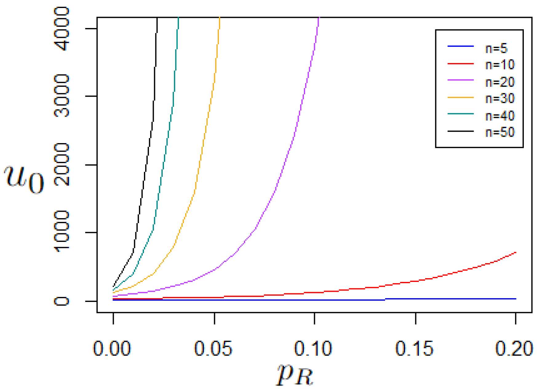
Next, we show how the expected waiting time $u_0$ depends on the probability $p_R$ for different values of n.

Note that the behavior of the expected waiting time $u_0$, depicted in Figure 1, is consistent with the intuition we have about CCPRB: $u_0$ increases as n increases (as having more standard coupons to collect extends the waiting time), and $u_0$ increases as $p_R$ increases (as resets remove the coupons already collected, and therefore extend the waiting time).

In some cases considered, we can also notice some kind of exponential growth, which we discuss in more detail in the next section.

5. Asymptotic Properties of the Waiting Times ${\mathbf{v}}_{\mathbf{1}}$ and ${\mathbf{u}}_{\mathbf{0}}$

Here, we analyze the properties of the expected waiting times until the end of the collection process, as the number of standard coupons n tends to infinity, for different values of the probability $p_R$. We can distinguish between the case when $p_R$ is fixed, and the case when $p_R$ depends on n.

For fixed $p_R\in (0,1)$, we can apply the Stirling approximation of the term $B\left(n,\frac{n{p}_R}{1-p_R}\right)$ in Theorem 3, and obtain the asymptotic estimate for $u_0$, as $n\to \infty$, formulated in the next proposition.

Proposition 1.

For any $p_R\in (0,1)$, the following asymptotic relation holds as $n\to \infty$:

$$u_0\sim \frac{1}{p_R}\left(\frac{1}{\sqrt{2p_R\pi n}{(1-p_R)}^n{p}_R^{\frac{n{p}_R}{1-p_R}}}-1\right).$$

(43)

Remark 5.

The expression (43) can be alternatively written in the following form:

$$u_0\sim \frac{1}{p_R}\left(\frac{{\alpha }^{-n}}{\sqrt{2p_R\pi n}}-1\right),\mathit{where}\alpha =(1-p_R)p_R^{\frac{p_R}{1-p_R}}.$$

(44)

The relations (43) and (44) also hold when $p_R$ depends on n, in the case when the ratio $\frac{n{p}_R}{1-p_R}=\frac{p_R}{p}$ tends to infinity as $n\to \infty$.

For the case when the ratio $\frac{n{p}_R}{1-p_R}$ is bounded (which means that the collection process is not interrupted too often by resets), we have the following asymptotic result.

Proposition 2.

For $\frac{n{p}_R}{1-p_R}=O\left(1\right)$, the following asymptotic relation holds, $n\to \infty$:

$$u_0\sim \frac{1}{p_R}\left(\frac{n^{\frac{n{p}_R}{1-p_R}}}{(1-p_R)\mathsf{\Gamma }(\frac{n{p}_R}{1-p_R}+1)}-1\right).$$

(45)

Proof. 

The statement follows from Theorem 3 and the relation

$$\underset{x\to \infty }{lim}\frac{\mathsf{\Gamma }(x+a)}{x^{a-b}\mathsf{\Gamma }(x+b)}=1$$

(46)

(see, for example, [19], page 257). □

Next, we analyze some particular cases of the problem.

Example 3.

The case $p_R=p=\frac{1}{n+1}$ corresponds to the situation where the reset coupon has the same probability of being drawn as any other coupon. Using Theorem 3, we obtain the expressions

$$v_1=(n+1)(1-B(n,1))=\frac{n^2-1}{n}\sim n,\mathrm{as}n\to \infty ,$$

(47)

and

$$u_0=(n+1)\left(\frac{1}{\frac{n}{n+1}B(n,1)}-1\right)=n(n+1)\sim n^2,\mathrm{as}n\to \infty .$$

(48)

This case is “exactly solvable", in the sense that, for a given value $u_0$, we can simply obtain $n=n_{u_0}$ such that the expected waiting time is less or equal to $u_0$. Precisely, from the inequality

$$n^2+n\le u_0$$

and the fact that $n_{u_0}\ge 0$, we obtain that

$$n_{u_0}\in \left[0,\frac{-1+\sqrt{1+4u_0}}{2}\right].$$

Example 4.

The case $p_R=\frac{1}{2}$ corresponds to the situation where the ratio $\frac{n{p}_R}{1-p_R}$ is equal to n. Using Theorem 3, we obtain the expressions

$$v_1=2(1-B(n,n))\sim 2\left(1-\frac{\sqrt{\pi n}}{2^{2n-1}}\right),\mathrm{as}n\to \infty ,$$

(49)

and

$$u_0=2\left(\frac{2}{nB(n,n)}-1\right)\sim 2\left(\frac{2^{2n}}{\sqrt{\pi n^3}}-1\right),\mathrm{as}n\to \infty .$$

(50)

6. Conclusions

In this paper, we considered a generalization of the coupon collector problem where there is an additional coupon that resets the collection process and is drawn with probability $0\le p_R<1$.

We distinguished between cases where standard coupons are drawn with arbitrary probabilities that sum up to $1-p_R$ (which generalizes CCPU), and the case where standard coupons are drawn with the same probability $\frac{1-p_R}{n}$ (which generalizes CCP). The object of interest was the waiting time until the end of the coupon collection procedure.

For the case of equal probabilities, we specified the distribution of this waiting time in a very general way, in terms of the corresponding distribution in CCPU.

For the case of equal probabilities, applying the first step analysis for the appropriately constructed Markov chains, we have obtained the expression for the expected waiting time in both possible cases (when the collection process continues after the reset or not), and derived its simple form in terms of the beta function. We determined the asymptotic behavior (when the size of the collection tends to infinity) of the expected waiting time, considering possible values of the probability $p_R$ (fixed or depending on n).

We have also discussed some characteristic examples of this problem.

The possible applications (or interpretations) of this work relate to the detection of distributed denial-of-service (DDoS) attacks, which are explained, for example, in [5]. The authors conclude that, since the solution to these attacks is to continuously monitor Internet traffic, the occurrence of standard coupons in the coupon collector problem corresponds to tracking c (out of n) recent high traffic flows, where the portion size c is determined by server capacity, and the probability of null coupon, $p_N$, corresponds to the case of flows with small probabilities that sum up to $p_N$. In this context, the appearance of the reset coupon at the moment $t_0$ can be interpreted as a system crash, which leads to losing information about high traffic flows that have been monitored up to that moment. Having information about the frequency of such crashes is important for maintaining proper protection.