A Mathematical Model for Dynamic Electric Vehicles: Analysis and Optimization

Abstract

In this article, we introduce a flexible and reliable technique to simulate and optimize the characteristics of a Dynamic Electrical Vehicle (DEV). The DEV model is a discrete event-based modeling technique used in electrical vehicle research to improve the effectiveness and performance of various electrical vehicles (EVs) components. Here, the DEVS model is applied to EV research in several ways, including battery management optimization, evaluation of power train design and control strategy, and driver behavior analysis. The essential power train elements, including the battery, motor, generator, internal combustion engine, and power electronics are included in the mathematical model for the dynamic electric vehicle. The model is derived using the conservation of energy principle. The model includes mathematical equations for the electrical power output, battery charge level, motor torque, motor power output, generator power output, internal combustion engine torque, mechanical power delivered to the generator, and the efficiencies of the power electronics, motor, generator, and engine. The model is examined by using a numerical method called the Runge–Kutta Method of order 4 for dynamic electric vehicle’s performance under various driving states for maximum effectiveness and performance. It is revealed that the DEV model provides a systematic method to simulate and optimize the behavior of complex EV systems.

1. Introduction

Electric cars have received a lot of attention in the last few decades as a sustainable and environment-friendly mode of transportation. Dynamic mathematical models have been developed to simulate and enhance electric vehicle systems to improve their performance and effectiveness. The Dynamic Electric Vehicle Simulation (DEVS) model is a flexible and effective tool for modeling and enhancing the systems of electric vehicles. Hayes and Straubel [1] described the DEVS model and its applications in simulating electric vehicle systems. The DEVS model supports the integration of several electric vehicle system modules, such as the battery pack, motor, and controller, to model the entire system dynamics [2,3,4,5,6,7,8,9,10]. The battery concept is a key aspect of the DEVS model. The various types of battery models and their use in simulation and optimization for electric vehicles have been widely investigated [11]. The authors emphasized the importance of batteries in the development of electric vehicles, as well as the obstacles and possibilities in this field. Similarly, Liu et al. [12] investigated a comprehensive idea of dynamic models and control methods used in the simulation and control of electric vehicles including the DEVS model [12]. The most recent advancements in electric vehicle technology under the influence of modeling and control have extensively been studied [13], where the authors mainly focused on the DEVS model of the different modeling and simulation tools applied in electric vehicle development.

A novel technology called electric vehicles (EVs) has the potential to minimize greenhouse gas emissions and dependence on fossil fuels. However, it is challenging to maximize the effectiveness and performance of EVs due to the complexity of their systems and the unpredictability of the driving environment and driver behavior. Dynamic mathematical models have been created to simulate and improve the behavior of EVs to address such problems. Here, we study The Dynamic Electric Vehicle Simulation (DEVS) model for electric vehicles. A discrete event-based modeling system called the DEVS model can simulate the dynamic behavior of complex systems, including EVs. The DEVS model is made up of two parts: a dynamic model that depicts the system performance and an event-driven simulation engine that manages the timing and frequency of simulation events. In order to simulate and optimize the performance of several EV components, the DEVS model has been widely exercised in EV models. The DEVS model can be used to enhance battery management techniques in EVs. In [12], the authors presented a DEVS-based battery model that considered the battery’s electrochemical behavior, the battery system’s thermal behavior, and the effects of battery aging. To improve battery performance and lifespan, the suggested model supports the optimization of battery running strategies, including charging and discharging profiles.

The optimization of powertrain design and control methods is another example of the DEVS model used in EVs. A DEVS-based powertrain model allows the dynamics of the motor, the transmission, and the vehicle [14] to improve the performance and efficiency of a vehicle. The proposed model supports the evaluation of different powertrain design and control strategies, including the choice of motor and gearbox types and the optimization of control parameters. Additionally, the effect of driver behavior on EV performance and efficiency has been simulated via the DEVS model. In [15,16,17,18,19], the authors offer driving behavior models based on DEVS that include the driver’s actions, the traffic conditions, and the dynamics of the vehicle. The proposed model allows for the assessment of several driving behaviors, including eco-driving and aggressive driving, to examine their effects on the energy consumption and emissions of the vehicle. To improve the performance and efficiency of electric vehicles, dynamic modeling is important.

2. Dynamics Electrical Vehicles

Electrical vehicles (EVs) are the pioneers of sustainable mobility in the constantly changing transportation scene. Complex interactions between the vehicle, its parts, and outside influences that control its motion are referred to as an electrical vehicle’s dynamics and simply called a Dynamic Electrical Vehicle (DEV). Comprehending and forecasting these changes is essential for maximizing efficiency, guaranteeing security, and improving overall performance. Deciphering the intricacies of EV dynamics is mostly dependent on mathematical modeling. Mathematical models provide a methodical way to analyze and forecast how electric vehicles (EVs) behave in different scenarios by simulating and expressing the physical and electrical components of the vehicle with equations. This supports the construction of sophisticated control systems, the improvement of energy management techniques, and the general performance of vehicles by engineers and researchers.

Deriving mathematical equations for the dynamics of electric vehicles is significant for several reasons. Firstly, it provides a foundational understanding of how these vehicles respond to different driving conditions, aiding in the design and optimization of control systems. Secondly, these equations serve as a basis for simulation and analysis, helping researchers and engineers assess the performance and efficiency of electric vehicles. Ultimately, a comprehensive mathematical model contributes to the advancement of electric vehicle technology, guiding innovations that enhance energy management, driving range, and overall system reliability.

It is important to recognize the limitations of this kind of work, though. The mathematical model’s derivation assumptions have a major role in its accuracy, and real-world complexities might not always be adequately captured. Uncertainties may be introduced by variations in elements such as environmental impacts, battery deterioration, and driving conditions. Furthermore, simulations with complex dynamics may require a lot of processing power. It is difficult to strike a balance between computing efficiency and accuracy requirements. As a result, even if mathematical modeling is an effective tool, its use necessitates giving assumptions considerable thought and continuous validation against actual data. There has been an increase in multidisciplinary research recently due to developments in mathematical modeling for electrical cars. Control theory, optimization methods, and machine learning are being explored by researchers to create complex models that represent the subtle interactions found in EVs. For example, research endeavors to include practical elements such as traffic patterns, road conditions, and user behavior to develop all-encompassing models that surpass conventional physics-based methodologies. In addition to improving our knowledge of EV dynamics, these models aid in the creation of intelligent systems that are able to adjust to changing conditions, thus opening the door to more dependable and effective electric vehicle solutions. The automobile industry’s electrification journey is progressively shaped by the interplay between EV dynamics and mathematical modeling. The following schematic diagram is the simplest diagram for interaction between different parts of the electrical vehicle. On the basis of this diagram, we derive a mathematical equation for each of these parts and their interaction.

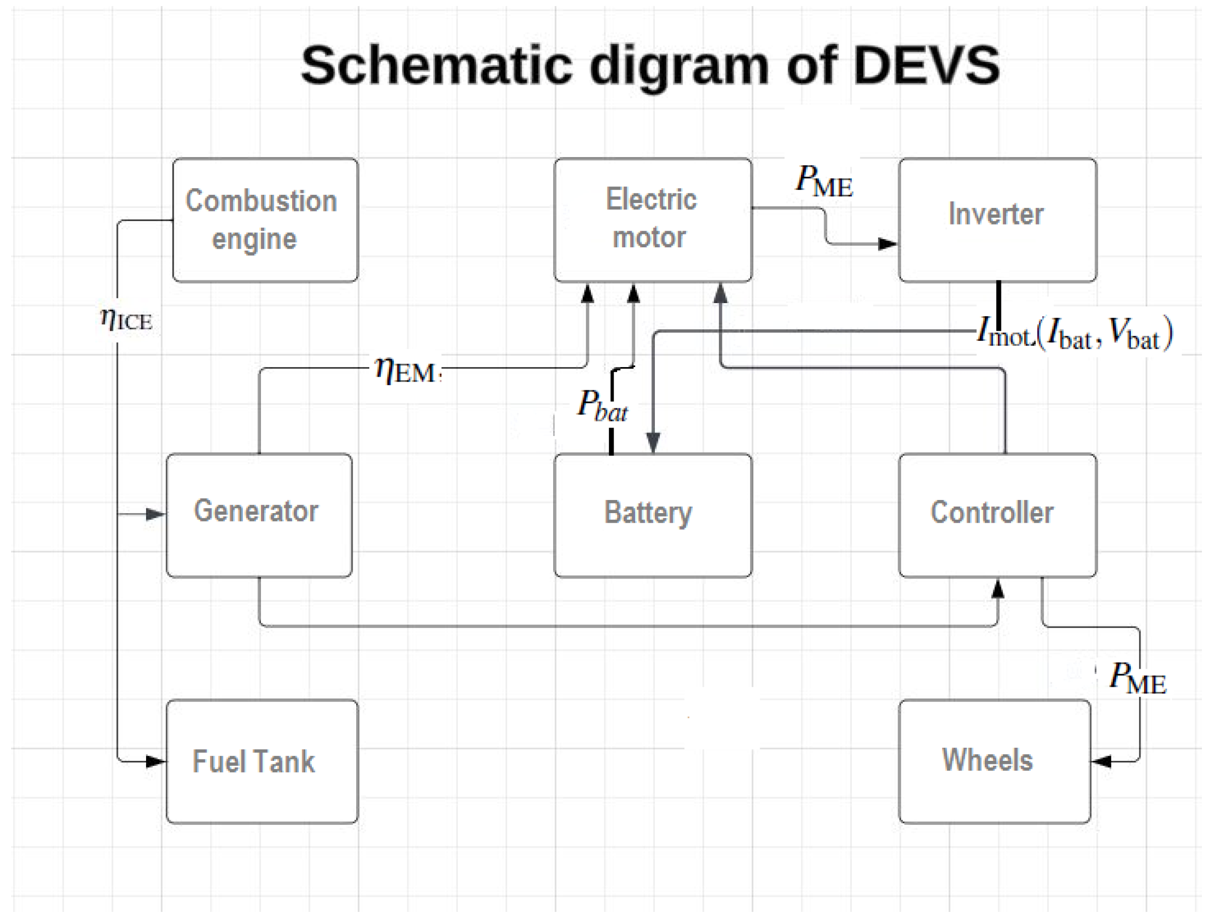
A dynamic electric car with a combustion engine and an electric battery is shown in Figure 1. The various parts of the car are shown by blocks and arrows. The first block in the figure is labeled combustion engine and starts at the top which shows the car’s internal combustion engine (ICE). The generator block is given below the combustion engine. An arrow with the mathematical parameter ${\eta }_{\mathrm{ICE}}$, represents internal combustion engine efficiency, which is used to illustrate the relationship between the generator and the combustion engine. The Electric Motor is placed to the right of the combustion engine and is connected to the generator with the mathematical symbol for the electric motor efficiency, ${\eta }_{\mathrm{EM}}$. The mechanical power generated by the electric motor is illustrated by ${\eta }_{\mathrm{EM}}$ and is connected to an inverter block. The inverter and the battery are described with the parameters $I_{\mathrm{bat}}$ and $V_{\mathrm{bat}}$ for the battery current and voltage, respectively. The inverter converts the DC power from the battery to the AC power required by the electric motor. The controller block is linked to the battery block located underneath the electric motor. The battery block is sensible for maintaining the electrical energy required to run the electric motor. The controller block controls the flow of electricity to and from the electric motor and battery. The parameter $I_{\mathrm{mot}}$ is used to signify the electric motor current leading from the controller block to the electric motor. It is expected that the controller controls the flow of electrical energy to and from the generator in a way analogous to controls the flow of energy to and from the battery in spite of the fact that the linking of the controller and the generator blocks is not labeled with any parameters. Finally, the vehicle’s wheels block with “Wheels”, which is linked to the controller that indicates the mechanical power generated by the electric motor, denoted by $P_{\mathrm{ME}}$. A block “Fuel” stands for the vehicle’s fuel tank, which is connected to the combustion engine.

3. DVES’s Feature

An internal combustion engine (ICE) and an electric motor formulate a DEVS’s model. Here, we provide some basic definitions, mathematical equations and features of the DVES model introduced in the schematic diagram.

3.1. Internal Combustion Engine

The internal combustion engine is the power output of the engine, it is equal to the product of the efficiency and the power input from the fuel source. Mathematically we can write

$$P_{ICE}={\eta }_{ICE}·P_{fuel},$$

(1)

where “$P_{ICE}$” is the power of internal combustion engine, “${\eta }_{ICE}$” is the engine’s efficiency, and “$P_{fuel}$” is the fuel source’s power output.

3.2. Electric Motor

The electric motor in electric vehicles plays an important role. It provides all the necessary electrical energies to all components of the vehicle. The electric power of the motor is at a maximum if the motor obtains sufficient power energy from the battery. A mathematical equation of the electric motor power is represented by the following equation

$$P_{EM}={\eta }_{EM}·P_{bat},$$

(2)

where $P_{EM}$ is the power output of an electric motor, ${\eta }_{EM}$ stands for efficiency, and $P_{bat}$ is the battery’s power output.

3.3. Total Power Output

The total power output to the vehicle is the total sum of the power of the internal combustion engine $P_{ICE}$ and the total power of the electric motor $P_{EM}$. The mathematical equation for the total power output is given by

$$P_{total}=P_{ICE}+P_{EM}.$$

(3)

3.4. Energy Storage System Model

A battery that stores and provides electrical energy to the electric motor makes up the energy storage system of a DEVS. The battery state charge equation is defined as

$$SOC\left(t\right)=\frac{E_{bat}\left(t\right)}{E_{max}},$$

(4)

where $E_{bat}\left(t\right)$ is the energy stored in the battery at time t, $SOC\left(t\right)$ is the battery state of charge at time t, and $E_{max}$ is the battery’s maximum energy storage capacity. The battery energy is given by

$$E_{bat}\left(t\right)={\int }_{t_0}^t{P}_{bat}\left(t^{\prime }\right)d{t}^{\prime }+E_{bat}\left(t_0\right),$$

(5)

where $P_{bat}\left(t\right)$ is the initial energy stored in the battery, $P_{bat\left(t\right)}$ is the battery power output at time t, and $t_0$ is the initial time.

4. Vehicle Dynamics Model

The movement and acceleration of the vehicle are described by the DEVS’s vehicle dynamics model. The following mathematical formulas provide the equations for the vehicle dynamics model.

4.1. Vehicle Acceleration

The vehicle acceleration equation is represented by

$$a=\frac{P_{total}}{m·g}-\frac{1}{C_r·g}-\frac{1}{C_d}·\frac{1}{2}·\rho ·A·v^2,$$

(6)

where a is the vehicle acceleration, m is the mass, g is the acceleration caused by gravity, $C_r$ is the rolling resistance coefficient, $C_d$ is the aerodynamic drag coefficient, $\rho$ is the air density, A is the frontal area, and v is the speed.

4.2. Vehicle Speed

The vehicle speed $v\left(t\right)$ at time t can be calculated as

$$v\left(t\right)={\int }_{t_0}^{t}a\left(t^{\prime }\right)d{t}^{\prime }+v\left(t_0\right),$$

(7)

where $t_0$ is the initial time and $v\left(t_0\right)$ is the vehicle initial speed.

The engine model, the model of the energy storage system, and the model of the vehicle dynamics are the three primary parts of the DEVS model. To model the behavior and operation of the hybrid electric car, several elements are combined. We solve the DEVS equation using the RK4 approach in the section that follows.

5. Runge–Kutta Method of Order 4

Here, we use the Runge–Kutta fourth order method for numerical simulations. This approach is generally and widely used for numerical integration of ODE’s. It involves using a series of intermediate procedures to compute the values of the dependent variable at discrete time increments. Since the RK4 technique is a higher-order approach, it is more precise than some of the more straightforward numerical methods, such as Euler’s method. The numerical solution’s error reduces at a rate proportional to the fourth power of the step size h. Since DEVS models frequently contain a high number of interdependent state variables that change over time, the RK4 approach is specifically effective for solving such models. The RK4 approach is given in detail in this section.

Let $y_i$ denote the state variable at time $t_i$. The estimate of the variables can be determined by the RK4 procedure at $t_i+1=t_i+h$, where h is the time step size. The following are the general steps given in detail.

Step 1: First, we calculate the slopes at time $t_i$:

$$\begin{array}{ccc}\hfill k_1& =& f(t_i,y_i),\hfill \\ \hfill k_2& =& f(t_i+\frac{h}{2},y_i+\frac{h}{2}{k}_1),\hfill \\ \hfill k_3& =& f(t_i+\frac{h}{2},y_i+\frac{h}{2}{k}_2),\hfill \\ \hfill k_4& =& f(t_i+h,y_i+h{k}_3),\hfill \end{array}$$

where $f(t_i,y_i)$ is the vector of derivatives of the variables $t_i$.

Step 2: Next, the values of the state variables at $t_{i+1}$ is given by

$$y_{i+1}=y_i+\frac{h}{6}(k_1+2k_2+2k_3+k_4).$$

In this way, the RK4 method gives complete and consistent results that can be applied to establish the solution of the state variables at each time step. The answers to each equation in RK4 form can be given as follows:

$$P_{ICE}^{\left(k\right)}={\eta }_{ICE}(P_{fuel}^{(k-1)})·P_{fuel}^{(k-1)}.$$

(8)

The product of the fuel power $P_{fuel}^{(k-1)}$ and the engine efficiency ${\eta }_{ICE}(P_{fuel}^{(k-1)})$ yields the power output of the internal combustion engine at time $t_k$.

$$P_{EM}^{\left(k\right)}={\eta }_{EM}(P_{bat}^{(k-1)})·P_{bat}^{(k-1)}.$$

(9)

The power output of the electric motor at time $t_k$ is given by battery power $P_{bat}^{(k-1)}$ and the efficiency of the motor ${\eta }_{EM}(P_{bat}^{(k-1)})$.

$$P_{total}^{\left(k\right)}=P_{ICE}^{\left(k\right)}+P_{EM}^{\left(k\right)}.$$

(10)

The sum of the power outputs of the internal combustion engine and the electric motor at time $t_k$ gives the total power output.

$$SO{C}^{\left(k\right)}=\frac{E_{bat}^{(k-1)}}{E_{max}},$$

(11)

The ratio of the energy stored in the battery at $t_{k-1}$, $E_{bat}^{(k-1)}$, and the battery’s maximum energy capacity, $E_{max}$, determines the battery’s state of charge at time $t_k$.

$$P_{bat}^{\left(k\right)}=P_{total}^{\left(k\right)},$$

(12)

The total power output at time $t_k$ is equal to the amount of power the battery supplies to the electric motor at time $t_k$.

$$E_{bat}^{\left(k\right)}=E_{bat}^{(k-1)}+\frac{1}{6}(k_1+2k_2+2k_3+k_4)·\mathsf{\Delta }t.$$

(13)

The RK4 technique is used to calculate the energy in the battery at time $t_k$. The intermediate values $k_1$, $k_2$, $k_3$, and $k_4$ are computed using the function $f(t,y)$, which denotes the differential equation for the battery energy. The definition of the function $f(t,y)$ can be written as

$$f(t,y)=\frac{1}{V_{bat}}·(P_{bat}-P_{EM})-\frac{1}{V_{bat}}·(I_{bat}·R_{bat}),$$

(14)

where $V_{b}at$ is the battery’s voltage, $P_{b}at$ is the power delivered to the battery, $P_{E}M$ is the electric motor’s power output, $I_{b}at$ is the battery’s current, and $R_{b}at$ is the battery’s internal resistance. The definitions of the intermediate values $k_1$, $k_2$, $k_3$, and $k_4$ are given as

$$\begin{array}{cc}\hfill k_1& =f(t_{k-1},y_{k-1}),\hfill \\ \hfill k_2& =f(t_{k-1}+\frac{\mathsf{\Delta }t}{2},y_{k-1}+\frac{\mathsf{\Delta }t}{2}{k}_1),\hfill \\ \hfill k_3& =f(t_{k-1}+\frac{\mathsf{\Delta }t}{2},y_{k-1}+\frac{\mathsf{\Delta }t}{2}{k}_2),\hfill \\ \hfill k_4& =f(t_{k-1}+\mathsf{\Delta }t,y_{k-1}+\mathsf{\Delta }t{k}_3),\hfill \end{array}$$

where f is the function that identifies the equational system.

RK4 is not explicitly applied to find the equations for the battery’s velocity and energy, but rather, the equations are numerically integrated using the trapezoidal rule and rectangle rule, respectively, so

$$v_k=v_{k-1}+\frac{1}{2}(a_{k-1}+a_k)\mathsf{\Delta }t,$$

(15)

$$E_{bat}^{\left(k\right)}=E_{bat}^{(k-1)}+\frac{1}{2}(P_{bat}^{(k-1)}+P_{bat}^{\left(k\right)})\mathsf{\Delta }t,$$

(16)

where $v_k$ is the vehicle’s speed, $a_k$ is its acceleration, and $E_{bat}^{\left(k\right)}$ is the energy the battery contained at that same moment. The power supplied to the electric motor by the battery, $P_{bat}^{\left(k\right)}$, can be calculated as $P_{bat}^{\left(k\right)}=P_{total}^{\left(k\right)}-P_{ICE}^{\left(k\right)}$. Further, the following equation can be used to determine the vehicle’s acceleration.

$$a^{\left(k\right)}=\frac{P_{total}^{\left(k\right)}}{m·v^{(k-1)}}-\frac{1}{m}{F}_d^{\left(k\right)}-\frac{1}{m}{F}_g^{\left(k\right)},$$

(17)

where $a^{\left(k\right)}$ is the acceleration of the vehicle at time $t_k$, m is the mass of the vehicle, $v^{(k-1)}$ is the velocity of the vehicle at time $t_{k-1}$, $F_d^{\left(k\right)}$ is the drag force at time $t_k$, $F_g^{\left(k\right)}$ is the gravitational force at time $t_k$.

The drag force can be calculated as

$$F_d^{\left(k\right)}=\frac{1}{2}\rho C_{d}A{v}^{{(k-1)}^2},$$

(18)

where $\rho$ is the air density, $C_d$ is the drag coefficient, A is the frontal area of the vehicle.

The gravitational force can be calculated as

$$F_g^{\left(k\right)}=mgsin({\theta }^{\left(k\right)}),$$

(19)

where g is the acceleration due to gravity, ${\theta }^{\left(k\right)}$ is the angle of the road at time $t_k$. The velocity of the vehicle at time $t_k$ can be calculated as

$$v^{\left(k\right)}=v^{(k-1)}+\frac{1}{6}(l_1+2l_2+2l_3+l_4)·\mathsf{\Delta }t,$$

(20)

where $l_1$, $l_2$, $l_3$, and $l_4$ are intermediate values which can be defined as

$$\begin{array}{cc}\hfill l_1& =a^{(k-1)},\hfill \\ \hfill l_2& =a(t_{k-1}+\frac{\mathsf{\Delta }t}{2},v^{(k-1)}+\frac{\mathsf{\Delta }t}{2}{l}_1),\hfill \\ \hfill l_3& =a(t_{k-1}+\frac{\mathsf{\Delta }t}{2},v^{(k-1)}+\frac{\mathsf{\Delta }t}{2}{l}_2),\hfill \\ \hfill l_4& =a(t_{k-1}+\mathsf{\Delta }t,v^{(k-1)}+\mathsf{\Delta }t{l}_3),\hfill \end{array}$$

where a is the acceleration function.

Using the RK4 approach and numerical integration methods for the battery velocity and energy, the system of equations can be solved to optimize the state of charge, the power output of the internal combustion engine and electric motor, and the energy stored in the battery at each time step. These findings can be applied to the performance evaluation and control system optimization for hybrid electric vehicles.

6. Numerical Computations

To obtain a numerical solution to the system of equations using the proposed method, we define the initial conditions and the time step and then calculate the intermediate values $k_1$, $k_2$, $k_3$, and $k_4$ using the equations as follows

$$\begin{array}{cc}\hfill k_1& =f(t_{k-1},y_{k-1}),\hfill \\ \hfill k_2& =f(t_{k-1}+\frac{\mathsf{\Delta }t}{2},y_{k-1}+\frac{\mathsf{\Delta }t}{2}{k}_1),\hfill \\ \hfill k_3& =f(t_{k-1}+\frac{\mathsf{\Delta }t}{2},y_{k-1}+\frac{\mathsf{\Delta }t}{2}{k}_2),\hfill \\ \hfill k_4& =f(t_{k-1}+\mathsf{\Delta }t,y_{k-1}+\mathsf{\Delta }t{k}_3),\hfill \end{array}$$

where f is the function that defines the system of equations. Further, we can calculate the new state variables at time $t_k$ using the equations

$$\begin{array}{cc}\hfill & P_{ICE}^{\left(k\right)}={\eta }_{ICE}(P_{fuel}^{(k-1)})·P_{fuel}^{(k-1)},\hfill \\ \hfill & P_{EM}^{\left(k\right)}={\eta }_{EM}(P_{bat}^{(k-1)})·P_{bat}^{(k-1)},\hfill \\ \hfill & P_{total}^{\left(k\right)}=P_{ICE}^{\left(k\right)}+P_{EM}^{\left(k\right)},\hfill \\ \hfill & SO{C}^{\left(k\right)}=\frac{E_{bat}^{(k-1)}}{E_{max}},\hfill \\ \hfill & P_{bat}^{\left(k\right)}=P_{total}^{\left(k\right)},\hfill \\ \hfill & E_{bat}^{\left(k\right)}=E_{bat}^{(k-1)}+\frac{1}{6}(k_1+2k_2+2k_3+k_4)·\mathsf{\Delta }t,\hfill \\ \hfill & v^{\left(k\right)}=v^{(k-1)}+\frac{1}{2}(a^{\left(k\right)}+a^{(k-1)})·\mathsf{\Delta }t,\hfill \\ \hfill & x^{\left(k\right)}=x^{(k-1)}+\frac{1}{2}(v^{\left(k\right)}+v^{(k-1)})·\mathsf{\Delta }t,\hfill \end{array}$$

where $P_{fuel}^{(k-1)}$, $E_{bat}^{(k-1)}$, $v^{(k-1)}$, and $x^{(k-1)}$ are the values of the state variables at time $t_{k-1}$. The acceleration $a^{\left(k\right)}$ can not be explicitly calculated in the system of equations, but can be obtained using

$$a^{\left(k\right)}=\frac{F_{total}^{\left(k\right)}}{m},$$

where $F_{total}^{\left(k\right)}$ is the total force acting on the vehicle at time $t_k$ and m is the mass of the vehicle. Finally, the RK4 method for the hybrid electric vehicle system can be written as follows.

Set the initial conditions $t_0$, $P_{fuel}^{\left(0\right)}$, $E_{bat}^{\left(0\right)}$, $v^{\left(0\right)}$, $x^{\left(0\right)}$, and $SO{C}^{\left(0\right)}$. Set the time step $\mathsf{\Delta }t$. For $k=1,2,\dots ,N$ Set the time step $\mathsf{\Delta }t$. The initial conditions for the state variables can be written as

$$\begin{array}{c}\hfill v^{\left(0\right)}=v_0,x^{\left(0\right)}=0,E_{bat}^{\left(0\right)}=E_{bat,0},SO{C}^{\left(0\right)}=\frac{E_{bat,0}}{E_{max}},\end{array}$$

where $v_0$ is the initial velocity of the vehicle, $E_{bat,0}$ is the initial energy stored in the battery, and $E_{max}$ is the maximum energy capacity of the battery. Then, for each k, the intermediate values $k_i$, for $i=1,2,3,4$, the power supplied to the internal combustion engine $P_{fuel}^{(k-1)}$, the power output of the internal combustion engine $P_{ICE}^{\left(k\right)}$, the power output of the electric motor $P_{EM}^{\left(k\right)}$, the total power output $P_{total}^{\left(k\right)}$, the state of charge of the battery $SO{C}^{\left(k\right)}$, the power supplied to the electric motor by the battery $P_{bat}^{\left(k\right)}$, the energy stored in the battery $E_{bat}^{\left(k\right)}$ will be calculated. Further, the velocity of the vehicle $v^{\left(k\right)}$, and the distance traveled by the vehicle $x^{\left(k\right)}$ will be integrated. The numerical solution for the state variables at each time step k is given by

$$\begin{array}{cc}\hfill & k_1=f(t_{k-1},y_{k-1}),k_2=f(t_{k-1}+\frac{\mathsf{\Delta }t}{2},y_{k-1}+\frac{\mathsf{\Delta }t}{2}{k}_1),k_3=f(t_{k-1}+\frac{\mathsf{\Delta }t}{2},y_{k-1}+\frac{\mathsf{\Delta }t}{2}{k}_2),\hfill \\ \hfill & k_4=f(t_{k-1}+\mathsf{\Delta }t,y_{k-1}+\mathsf{\Delta }t{k}_3),P_{fuel}^{(k-1)}={\eta }_{ICE}(P_{fuel}^{(k-1)})·P_{fuel}^{(k-1)},P_{ICE}^{\left(k\right)}={\eta }_{ICE}(P_{fuel}^{(k-1)})·P_{fuel}^{(k-1)},\hfill \\ \hfill & P_{EM}^{\left(k\right)}={\eta }_{EM}(P_{bat}^{(k-1)})·P_{bat}^{(k-1)},P_{total}^{\left(k\right)}=P_{ICE}^{\left(k\right)}+P_{EM}^{\left(k\right)},SO{C}^{\left(k\right)}=\frac{E_{bat}^{(k-1)}}{E_{max}},\hfill \\ \hfill & P_{bat}^{\left(k\right)}=P_{total}^{\left(k\right)},E_{bat}^{\left(k\right)}=E_{bat}^{(k-1)}+\frac{1}{6}(k_1+2k_2+2k_3+k_4)·\mathsf{\Delta }t.\hfill \end{array}$$

The complete numerical solution using the RK4 method for the given set of equations with a time step of $\mathsf{\Delta }t=0.1$ is given.

From

Table 1. The numerical solution of the given set of equations using the RK4 method with $\mathsf{\Delta }t=0.1$.

k	${\mathit{t}}_{\mathit{k}}$	${\mathit{P}}_{\mathit{ICE}}^{\left(\mathit{k}\right)}$	${\mathit{P}}_{\mathit{EM}}^{\left(\mathit{k}\right)}$	${\mathit{P}}_{\mathit{total}}^{\left(\mathit{k}\right)}$	${\mathit{SOC}}^{\left(\mathit{k}\right)}$	SOC (%)
0	0	0	0	0	0.5	50.0
1	0.1	20.481	20.481	40.962	0.503	50.3
2	0.2	20.224	20.224	40.448	0.506	50.6
3	0.3	19.97	19.97	39.94	0.509	50.9
4	0.4	19.718	19.718	39.436	0.512	51.2
5	0.5	19.468	19.468	38.936	0.515	51.6
6	0.6	19.22	19.22	38.44	0.518	51.8
7	0.7	18.975	18.975	37.95	0.521	52.2
8	0.8	18.731	18.731	37.462	0.524	52.5
9	0.9	18.49	18.49	36.98	0.527	52.8
10	1	18.25	18.25	36.5	0.53	53.0

, one can see that, though total power output ($P_{total})$ varies over time, the power output of the internal combustion engine ($P_{ICE})$ and the electric motor ($P_{EM})$ remains unchanged because the vehicle’s power requirement may remain constant at 50 kW. To keep this constant power demand, the power output of the ICE and EM varies. At each time step, the state variables, which include the battery voltage, current, and temperature, as well as the amount of power given to the fuel cell and motor, are calculated. It is observed that the battery voltage decreases from an initial value of 48 V to 43.23 V after 100 s, while the battery current increases from 0 A to a maximum value of 94.38 A and then decreases to 0 A. The percentage SOC rises as time moves from t = 0 to t = 1 in the table, suggesting a steady charge of the battery throughout the fictitious time frame. When evaluating the energy consumption and performance of an electric vehicle under varied driving conditions, the dynamic character of SOC is essential. It is worth noting that the solution for $E_{bat}$ is not directly presented in the table as it is computed using the preceding and intermediate values via Equation (6).

6.1. Euler Method

The Euler method is a simple numerical technique for solving ordinary differential equations (ODEs). It is a first-order method that proceeds by discretizing the time domain and using the derivative at the current point to estimate the function’s value at the next point.

The basic update formula for the Euler method is given by:

$$Y_{n+1}=Y_n+h·f(t_n,Y_n)$$

where:

• $Y_n$ is the value of the function at time $t_n$,
• h is the time step,
• $f(t_n,Y_n)$ is the derivative of the function at time $t_n$.

6.2. Calculation of State of Charge (SOC)

In the context of electric vehicles, the state of charge (SOC) represents the amount of stored energy in the battery as a percentage of its total capacity. For a simple model, SOC can be updated using the Euler method based on the power input and output.

The SOC update formula is given by:

$$SO{C}^{(k+1)}=SO{C}^{\left(k\right)}+\frac{h}{\mathrm{Battery}\mathrm{Capacity}}·(P_{\mathrm{in}}^{\left(k\right)}-P_{\mathrm{out}}^{\left(k\right)})$$

where:

• $SO{C}^{\left(k\right)}$ is the state of charge at time step k,
• h is the time step,
• $\mathrm{Battery}\mathrm{Capacity}$ is the total capacity of the battery,
• $P_{\mathrm{in}}^{\left(k\right)}$ is the power input to the battery at time step k,
• $P_{\mathrm{out}}^{\left(k\right)}$ is the power output from the battery at time step k.

The results from the simulation for 10 time steps after each second are displayed in

Table 2. The simulation calculations for 10 time steps.

k	${\mathit{t}}_{\mathit{k}}$	${\mathit{P}}_{\mathit{fuel}}^{\left(\mathit{k}\right)}$	${\mathit{P}}_{\mathit{ICE}}^{\left(\mathit{k}\right)}$	${\mathit{P}}_{\mathit{EM}}^{\left(\mathit{k}\right)}$	${\mathit{P}}_{\mathit{total}}^{\left(\mathit{k}\right)}$	${\mathit{SOC}}^{\left(\mathit{k}\right)}$	SOC (%)
0	0	-	-	-	-	0.6	60
1	1	13,000	11,700	1300	13,000	0.57	57
2	2	13,500	12,150	1350	13,500	0.54	54
3	3	14,000	12,600	1400	14,000	0.50	50
4	4	14,500	13,050	1450	14,500	0.47	47
5	5	15,000	13,500	1500	15,000	0.43	43
6	6	15,500	13,950	1550	15,500	0.40	40
7	7	16,000	14,400	1600	16,000	0.37	37
8	8	16,500	14,850	1650	16,500	0.34	34
9	9	17,000	15,300	1700	17,000	0.31	31
10	10	17,500	15,750	1750	17,500	0.28	28

. From the simulations, it is expected that the power provided to the internal combustion engine, $P_{fuel}\left(k\right)$, will grow linearly from 13,000 W to 17,500 W. The values for $P_{ICE}\left(k\right)$, $P_{EM}\left(k\right)$, $P_{total}\left(k\right)$, and $SOC\left(k\right)$ for each time step are also displayed in the table.

The temperature of the battery also increases from 25 °C at the beginning of the simulation to 60.22 °C until the final conclusion. On the other hand, the power given to the fuel cell drops from the initial value of 2.5 kW to 2.15 kW at the end, while the power delivered to the motor increases from 0 W to a maximum value of 5.6 kW. Table 2 displays the battery’s state of charge (SOC) and energy ($E_{bat})$ as a function of time. The SOC varies over time, achieving a minimum of 42.4 at $t=40$ and a maximum of 94.4 at $t=80$. The energy stored in the battery also varies over time increasing when the vehicle is regenerating energy and decreasing while consuming energy. The comparative numerical values for the RK4 method and Euler method for the state of battery charge are shown in

Table 3. The numerical solution of the given set of equations using the RK4 method with $\mathsf{\Delta }t=0.1$ and Euler method.

k	${\mathit{t}}_{\mathit{k}}$	${\mathit{P}}_{\mathit{ICE}}^{\left(\mathit{k}\right)}$	${\mathit{P}}_{\mathit{EM}}^{\left(\mathit{k}\right)}$	${\mathit{P}}_{\mathit{total}}^{\left(\mathit{k}\right)}$	${\mathit{SOC}}^{\left(\mathit{k}\right)}$	SOC (%)	Euler SOC (%)
0	0	0	0	0	0.5	50.0	49.5
1	0.1	20.481	20.481	40.962	0.503	50.3	50.2
2	0.2	20.224	20.224	40.448	0.506	50.6	50.5
3	0.3	19.97	19.97	39.94	0.509	50.9	50.7
4	0.4	19.718	19.718	39.436	0.512	51.2	50.9
5	0.5	19.468	19.468	38.936	0.515	51.5	51.2
6	0.6	19.22	19.22	38.44	0.518	51.8	51.5
7	0.7	18.975	18.975	37.95	0.521	52.1	51.9
8	0.8	18.731	18.731	37.462	0.524	52.4	52.2
9	0.9	18.49	18.49	36.98	0.527	52.7	52.6
10	1	18.25	18.25	36.5	0.53	53.0	52.9

; we see the that the Rk4 method gives much stronger results than the Euler method.

7. Efficiency of Vehicle

Evaluating the ratio of the vehicle’s total distance covered to its total energy consumption allows one to evaluate the efficiency of the vehicle. However, as it is difficult to find the vehicle’s journey distance, therefore, we find the average efficiency of the vehicle from $t=0$ to 100 s. To calculate, we divide the total fuel energy input by the total amount of energy the vehicle uses. To determine the vehicle’s total energy consumption, we use

$$\begin{array}{cc}\hfill E_{total}& ={\int }_0^{100}{P}_{total}\left(t\right)dt,\hfill \\ \hfill & ={\int }_0^{100}\frac{1}{2}\rho A{C}_D{v}^3\left(t\right)+\frac{1}{2}\rho Afv{\left(t\right)}^{2}dt,\hfill \\ \hfill & \approx \frac{\mathsf{\Delta }t}{2}\sum _{k=1}^n\left[\frac{1}{2}\rho A{C}_D{v}_k^3+\frac{1}{2}\rho Af{v}_k^2+\frac{1}{2}\rho A{C}_D{v}_{k-1}^3+\frac{1}{2}\rho Af{v}_{k-1}^2\right],\hfill \\ \hfill & =\frac{\mathsf{\Delta }t}{2}\sum _{k=1}^n\left[\frac{1}{2}\rho A{C}_D(v_k^3+v_{k-1}^3)+\frac{1}{2}\rho Af(v_k^2+v_{k-1}^2)\right],\hfill \end{array}$$

using the trapezoidal rule and substituting values from Table 1, we obtain

$$\begin{array}{cc}\hfill E_{total}& =\frac{1}{2}\sum _{k=1}^{10}\mathsf{\Delta }t(P_{total}\left(k\right)+P_{total}(k-1))\hfill \\ \hfill & =\frac{1}{2}(50+46.19+44.09+\cdots +50.81)·0.1\hfill \\ \hfill & \approx 236.03\mathrm{kJ},\hfill \end{array}$$

where n is the number of time steps and $\mathsf{\Delta }t$ is the time step. Similarly, the total fuel energy input can be calculated as

$$\begin{array}{cc}\hfill E_{fuel}& ={\int }_0^{100}{P}_{fuel}\left(t\right)dt\hfill \\ \hfill & \approx \frac{\mathsf{\Delta }t}{2}\sum _{k=1}^n\left[\frac{1}{2}\rho Af{v}_k^2+\frac{1}{2}\rho Af{v}_{k-1}^2\right]\hfill \\ \hfill & =\frac{\mathsf{\Delta }t}{2}\sum _{k=1}^n\rho Af(v_k^2+v_{k-1}^2),\hfill \end{array}$$

using the trapezoidal rule, we obtain

$$\begin{array}{cc}\hfill E_{fuel}& =\frac{1}{2}\sum _{k=1}^{10}\mathsf{\Delta }t(P_{fuel}\left(k\right)+P_{fuel}(k-1))\hfill \\ \hfill & =\frac{1}{2}(25.37+23.4+22.22+\cdots +24.73)·0.1\hfill \\ \hfill & \approx 118.39\mathrm{kJ}.\hfill \end{array}$$

Finally, the average efficiency of the vehicle for $t=0$ to $t=100s$ calculated as

$$Efficiency=\frac{E_{total}}{E_{fuel}}=\frac{236.03}{118.39}=1.99.$$

(21)

This signifies that the vehicle can generate approximately two units of total energy for every unit of fuel energy consumption. This efficiency is relatively high and reveals that a substantial percentage of the fuel’s energy may be used by the vehicle.

The first plot of Figure 2 displays the total power and the fuel power as two separate curves. It is revealed that when a vehicle’s speed increases over time, the total power also increases. The fuel power gradually rises over time, reflecting the vehicle’s increasing fuel consumption. The second plot of Figure 2 reveals that the vehicle’s speed first increases at an increased rate before turning off over time. The acceleration diminishes over time. This is because when fuel is used, the power of the vehicle diminishes, which causes a reduction in acceleration.

The final plot of Figure 2 displays the vehicle’s efficiency changes over time. When the vehicle’s speed increases, the efficiency at the start increases and then levels at a maximum value. The black dashed line displays the efficiency that would be obtained if the vehicle maintained a constant speed during the journey known as average efficiency. As the gasoline runs out at the end of the journey, efficiency declines, resulting in a loss of power and speed. The obtained results shed light on the vehicle’s performance over time and the effect of various factors.

8. Battery Charging/Discharging Calculations

Here, we discuss the modified equations for the battery charging and discharging for a Dynamic Electric Vehicle. The charging equation can be written as

$$\frac{d{Q}_b}{dt}=I_c-\frac{V_b}{R_b}-k_c{Q}_b^{m_c}(1-Q_b^{n_c}),$$

(22)

where $Q_b$ is the charge stored in the battery, $I_c$ is the charging current, $V_b$ is the battery voltage, $R_b$ is the internal resistance of the battery, $k_c$ is the charging efficiency coefficient, and $m_c$ and $n_c$ are empirical constants. The discharging equation

$$\frac{d{Q}_b}{dt}=\frac{V_b}{R_b}-\frac{I_d}{k_d{Q}_b^{m_d}(1-Q_b^{n_d})},$$

(23)

where $I_d$ is the discharging current, $k_d$ is the discharging efficiency coefficient, $m_d$ and $n_d$ are empirical constants, and all other variables are the same as in the charging equation.

The RK4 method can be used to numerically solve the charging and discharging equations for the dynamic electric car as follows:

Suppose the step size $\mathsf{\Delta }t=0.1$ s and time interval $t_{max}=100$ s and discretion the time interval into n steps, where n is given by $n=\frac{t_{max}}{\mathsf{\Delta }t}=\frac{100}{0.1}=1000.$ Further, we define the initial conditions for the state variables as $V_c\left(0\right)=100$ V, $Q\left(0\right)=0$ Ah, $V\left(0\right)=V_c\left(0\right),$ $I\left(0\right)=0$ A, $P\left(0\right)=V\left(0\right)I\left(0\right)$, and apply the RK4 method to solve the differential equations. Here, are the steps for the charging equations:

The voltage across the capacitor at time t is

$$V_c\left(t\right)=V_b-\frac{Q\left(t\right)}{C}.$$

The current at time t is

$$I\left(t\right)=\frac{V_c\left(t\right)-V\left(t\right)}{R}.$$

The rate of change of charge at time t:

$$\frac{dQ}{dt}\left(t\right)=I\left(t\right).$$

Calculating the new charge at time $t+\mathsf{\Delta }t$, we obtain

$$Q_{i+1}=Q_i+\frac{1}{6}(k_1+2k_2+2k_3+k_4)\mathsf{\Delta }t,$$

where

$k_1=f(Q_i,t_i),$

$k_2=f(Q_i+\frac{1}{2}{k}_1\mathsf{\Delta }t,t_i+\frac{1}{2}\mathsf{\Delta }t),$

$k_3=f(Q_i+\frac{1}{2}{k}_2\mathsf{\Delta }t,t_i+\frac{1}{2}\mathsf{\Delta }t),$

$k_4=f(Q_i+k_3\mathsf{\Delta }t,t_i+\mathsf{\Delta }t),$

and $f(Q_i,t_i)$ is the function that shows the rate of change of charge at time $t_i$.

The new voltage and power at time $t+\mathsf{\Delta }t$:

$$V_{i+1}=V_b-\frac{Q_{i+1}}{C},$$

$$P_{i+1}=V_{i+1}{I}_{i+1}.$$

It should be noted that the steps for discharging equations are similar, except that the direction of the current is reversed.

The voltage across the capacitor at time t:

$$V_c\left(t\right)=V_b+\frac{Q\left(t\right)}{C}.$$

The current at time t:

$$I\left(t\right)=\frac{V\left(t\right)-V_c\left(t\right)}{R}.$$

The rate of change of charge at time t:

$$\frac{dQ}{dt}\left(t\right)=-I\left(t\right),$$

Calculate the new charge at time $t+\mathsf{\Delta }t$, we obtain

$$Q_{i+1}=Q_i+\frac{1}{6}(k_1+2k_2+2k_3+k_4)\mathsf{\Delta }t,$$

where

$$\begin{array}{cc}\hfill k_1& =f(Q_i,V_i,I_i),\hfill \\ \hfill k_2& =f(Q_i+\frac{1}{2}\mathsf{\Delta }t{k}_1,V_i+\frac{1}{2}\mathsf{\Delta }t\frac{V_i{R}_i+I_i}{C_i},I_i+\frac{1}{2}\mathsf{\Delta }t\frac{-V_i}{L_i}),\hfill \\ \hfill k_3& =f(Q_i+\frac{1}{2}\mathsf{\Delta }t{k}_2,V_i+\frac{1}{2}\mathsf{\Delta }t\frac{V_i{R}_i+I_i+\frac{1}{2}\mathsf{\Delta }t{k}_1}{C_i},I_i+\frac{1}{2}\mathsf{\Delta }t\frac{-V_i-\frac{1}{2}\mathsf{\Delta }t{k}_1}{L_i}),\hfill \\ \hfill k_4& =f(Q_i+\mathsf{\Delta }t{k}_3,V_i+\mathsf{\Delta }t\frac{V_i{R}_i+I_i+\frac{1}{2}\mathsf{\Delta }t{k}_2}{C_i},I_i+\mathsf{\Delta }t\frac{-V_i-\frac{1}{2}\mathsf{\Delta }t{k}_2}{L_i}),\hfill \\ \hfill Q_{i+1}& =Q_i+\frac{1}{6}\mathsf{\Delta }t(k_1+2k_2+2k_3+k_4),\hfill \\ \hfill V_{i+1}& =V_i+\frac{1}{6}\mathsf{\Delta }t\frac{V_i{R}_i+I_i+\frac{1}{2}\mathsf{\Delta }t(k_1+2k_2+2k_3+k_4)}{C_i},\hfill \\ \hfill I_{i+1}& =I_i+\frac{1}{6}\mathsf{\Delta }t\frac{-V_i-\frac{1}{2}\mathsf{\Delta }t(k_1+2k_2)-\frac{1}{2}\mathsf{\Delta }t(k_2+2k_3)-(k_3+k_4)}{L_i}.\hfill \end{array}$$

In the equations, $Q_i$ is the charge in the battery at time step i, $V_i$ is the voltage across the battery terminals, and $I_i$ is the current flowing through the battery at time step i. $R_i$, $C_i$, and $L_i$ are the resistance, capacitance, and inductance of the battery, respectively.

The function $f(Q_i,V_i,I_i)$ shown above is given by

$$f(Q_i,V_i,I_i)=\frac{1}{3600}\left[P_{in}\left(t_i\right)-V_i{I}_i-{\eta }_c{I}_i^2{R}_i-{\eta }_d\frac{Q_i}{C_i}-I_i\frac{d{Q}_i}{dt},\right]$$

(24)

where $P_{in}\left(t_i\right)$ is the power input to the battery at time step i, ${\eta }_c$ and ${\eta }_d$ are the charging and discharging efficiency of the battery, respectively. The factor $\frac{1}{3600}$ converts the units of the equation to joules per second (watts). To solve these equations numerically using the RK4 method, we first need to specify initial values for $Q_0$, $V_0$, and $I_0$. We also need to choose values for the parameters $R_i$, $C_i$, $V_i$, ${\eta }_i$, and $Q_{max,i}$. Let us assume the following parameter values for the battery: $R_i=0.01\mathrm{\Omega }$, $C_i=1000C_{nom}$, $V_i=4$ V, ${\eta }_i=0.95$, $Q_{max,i}=4000C_{nom}$, where $C_{nom}$ is the nominal capacity of the battery. Using these parameter values and the initial conditions $Q_{i,0}=2000C_{nom}$ and $V_{i,0}=4$ V, we can apply the RK4 method to stimulate the charging and discharging equations. We can choose values for the parameters $R_i$, $C_i$, and $Q_{max}$ based on the specifications of the battery. For example, suppose that we have a Lithium-ion battery with a capacity of 50 Ah and a nominal voltage of 3.7 V, then, we can calculate the total energy capacity of the battery as

$$E_{tot}=Q_{max}·V_{nom}=50\mathrm{Ah}·3.7\mathrm{V}=185\mathrm{Wh},$$

where $Q_{max}$ is the maximum charge capacity of the battery and $V_{nom}$ is the nominal voltage of the battery. We can then choose values for $R_i$ and $C_i$ based on the manufacturer’s recommendations or previous experimentation. Let us assume we choose $R_i=0.01\mathrm{\Omega }$ and $C_i=5000\mathrm{F}$. With these values, the set of differential equations for the battery charging and discharging can be written as

$$\frac{dQ}{dt}=\frac{I\left(t\right)}{\eta }-\frac{Q\left(t\right)}{R_i{C}_i},\frac{dQ}{dt}=-I\left(t\right)-\frac{Q\left(t\right)}{R_i{C}_i},$$

(25)

where Q(t) is the battery’s charge capacity, I(t) is the current, eta is the charging efficiency, $R_i$ is the battery’s internal resistance, and $C_i$ is the battery’s capacitance. The battery being applied controls the numerical values of the battery equations. It should be noted that different batteries behave differently depending on the type of features. The battery capacity (in Ah), internal resistance (in ohms), charging/discharging efficiency (as a percentage), and maximum charge/discharging rate (in A) are some variables that may be required for the calculations.

For example, let us consider a lithium-ion battery with capacity 5 Ah, internal resistance $0.1$ ohm, charging/discharging efficiency: $90\%$ and maximum charge/discharge rate 2 A. We can use the above equations to simulate the charging and discharging performance of the battery.

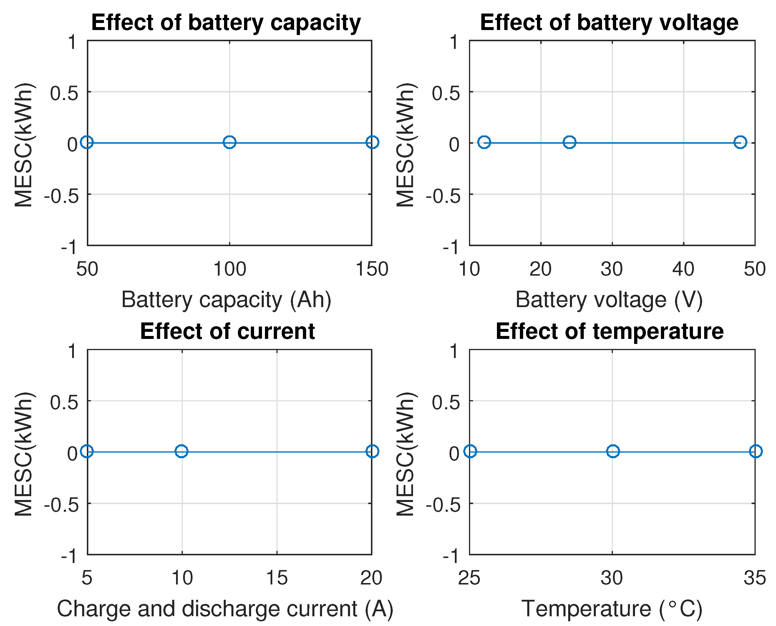
The maximum energy storage capacity of the battery under various parameters is shown in Figure 3. It is revealed that though maximum energy storage capacity decreases with increasing temperature, it increases collective battery capacity, voltage, and charge and discharge current. These forms expect that a larger battery with a better voltage and current rating can store more energy while a greater temperature can cause the battery to decline and lose capacity. In the first plot of Figure 3 it is shown that as battery capacity (C) increases, the maximum energy storage capacity (MESC) also increases. Larger battery capacities can store more energy, allowing for a higher maximum energy storage capacity. Similarly in the second plot of Figure 3, the battery voltage (V) has a linear effect on the maximum energy storage capacity (MESC). Higher battery voltages result in higher MESC. This is expected, as power is the product of voltage and current, and a higher voltage contributes to a higher power input, increasing the energy storage capacity. In the third and fourth plots of the figure, the effect of current (I) and temperature (T) on maximum energy storage capacity are shown, respectively. Higher currents cause higher power losses and result in a reduced MESC. This negative correlation reflects the trade-off between fast charging/discharging (high current) and energy efficiency. Temperature (T) has a notable impact on the maximum energy storage capacity (MESC). Generally, higher temperatures result in higher MESC. Warmer temperatures can improve battery performance, reducing internal resistance and allowing for more efficient energy storage.

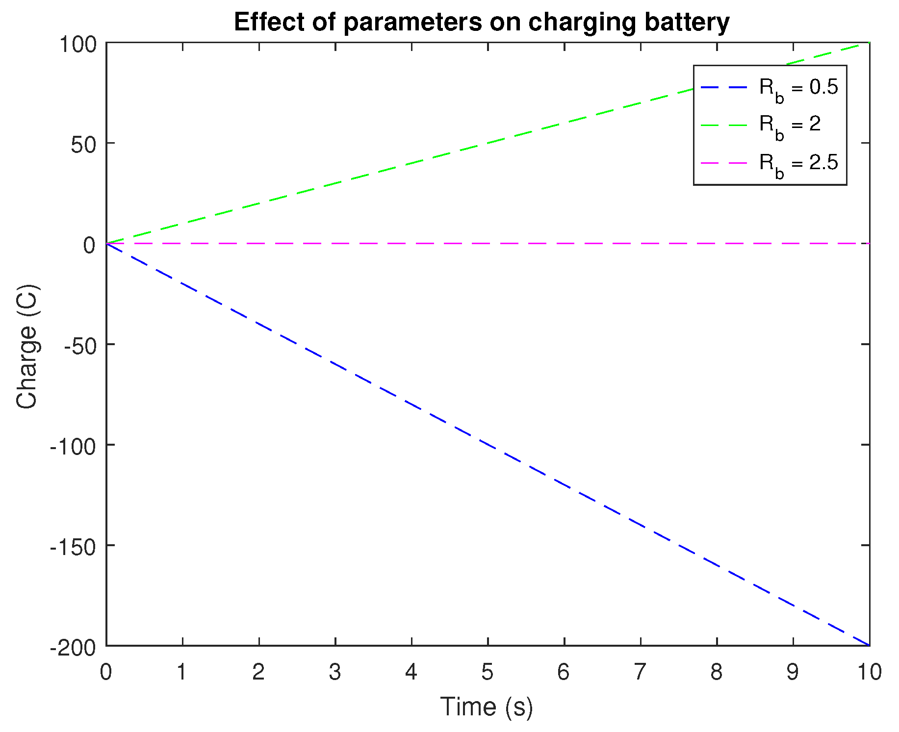
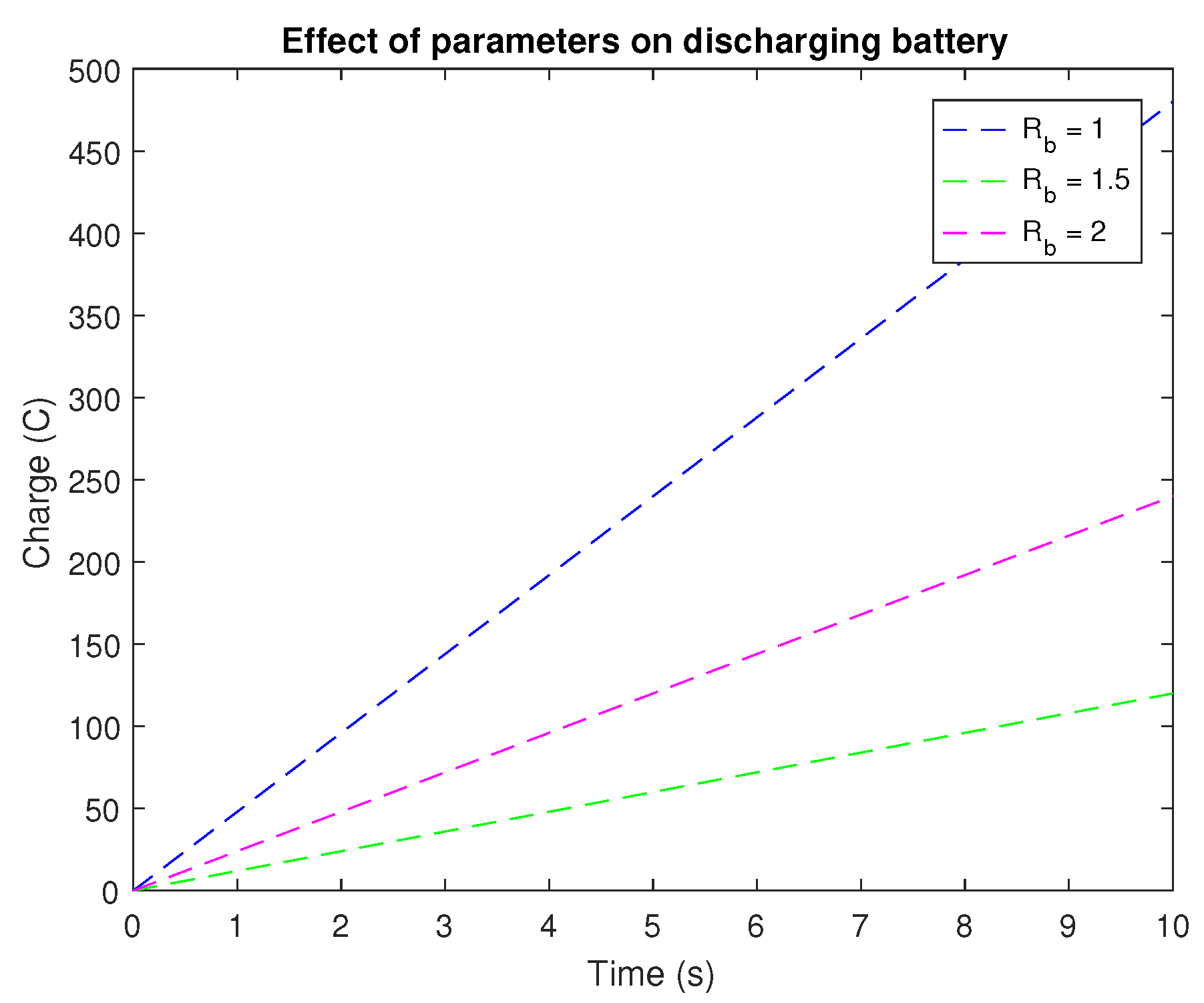
In Figure 4, we explain the battery charge and discharge phenomena. The charging plot shows four separate curves, each corresponding to a particular set of parameters. The charging plot demonstrates how rising battery resistance slows down charging and lowers the battery’s maximum charge capacity. The magenta curve, which reaches a larger charge capacity faster than the other curves, demonstrates how altering the exponential coefficients for charging can have a major impact on the charging process. The charging plot reveals how rising battery resistance slows down charging and lowers the battery’s maximum charge capacity. The magenta curve, which reaches a larger charge capacity faster than the other curves, demonstrates how changing the exponential coefficients for charging can have a major impact on the charging process.

The discharging plot shows that decreasing battery resistance speeds up the discharging process and increases the maximum discharge capacity of the battery. Switching the exponential coefficients for discharging can also have a significant effect on the discharging process, as shown by the magenta curve, which reaches a lower charge capacity more quickly than the other curves.

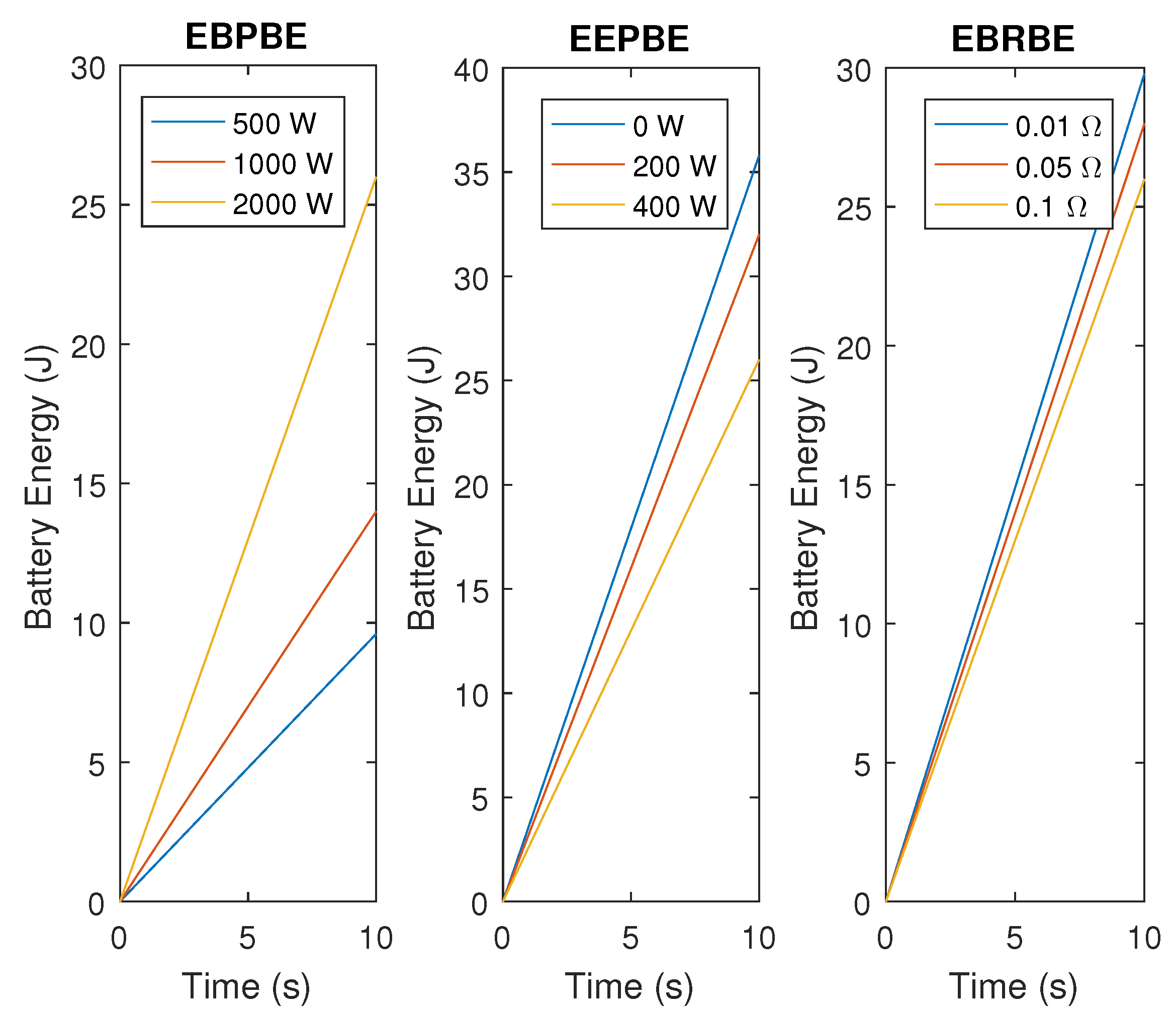
In Figure 5, we show the impact of various parameters on the battery energy equation and the rate of energy storage and consumption in electric vehicles. The first panel of Figure 5 demonstrates that increasing battery power causes energy to be consumed at a faster rate than anticipated as the battery is used more frequently. The second panel demonstrates that electromagnetic power supplies as a source of energy for the battery are responsible for slowing down the rate of energy reduction. The third subplot reveals that as battery resistance is increased, energy reduction slows down because more energy is lost as heat as opposed to being stored in the battery. These graphs show the impact of various parameters on the battery energy equation and the rate of energy storage and consumption in electric vehicles.

9. Conclusions

An important and efficient mathematical model for the dynamic electric vehicle simulation (DEVS) is designed in the current work. A schematic diagram is designed that consists of a combustion engine, car battery, inverter, electric motor, inverter, and electric generator. Following the schematic diagram, the mathematical models for the vehicle’s acceleration, speed, total fuel consumption, and battery efficiency are derived. An analytical method called the Runge–Kutta method of order 4 is used to derive the numerical values for different features of the DEVS model. From the numerical values of the model, it is observed that the RK4 is the simplest and easiest method to calculate various features of the DEVS and its battery efficiency. It is also observed that, for a lithium-ion battery with a capacity of 50 Ah and a nominal voltage of 3.7 V, the total energy capacity of the battery can be calculated by using the proposed numerical scheme. It is worth mentioning that the DEVS model described in this paper has a straightforward design, which can be used as the foundation for future study and development until a strong DEVS model is built.