Abstract
This paper extends the k-out-of-n:G reliability system to a multi-server queue. We study a multi-server reliability-queuing model with the N-policy of repair. The queuing system considered here has n servers, each of which has identically and exponentially distributed service times with parameter . Servers are subject to breakdown at an exponential rate . The repair process follows the N-policy of repair. Although these servers work independently of each other, service can be provided only when k functional servers are available in the system. We study the model in the steady state, using the matrix analytic method. We evaluate some associated performance measures and provide graphical/numerical illustrations. We consider an optimization problem, and the results of the study are presented.
MSC:
60K25; 60K10; 60K20; 90B22; 90B25
1. Introduction
This paper extends the reliability system k-out-of-n:G to a multi-server queue (n parallel server, with server failure and N-policy of repair). As in the k-out-of-n:G system, at least k servers should be operational in order for the whole system to work (system can provide service). At the moment that the number of operational servers is reduced to , the service is disrupted. As a result, the system can start operation only after one working server is added to the system. This model can be applied directly to the high-altitude platform (HAP) system used for smooth telecommunication when all other facilities fail, due to natural calamities. The system collapses when the number of operational servers is reduced to , irrespective of the number of customers in the system. As with parallel (at least one operational component should be UP for the system to function)/serial (all components should be operational for the system to be functional) systems in the reliability context, we encounter a similar situation in the queuing model discussed in this paper. Thus, this paper extends the k-out-of-n reliability system to the queuing system and simultaneously to the classical multi-server queuing system. In the proposed queuing model, an element of dependency on the number of operational servers arises. Thus, it differs from the classical multi-server queuing models in that at least k ( for the classical multi-server system with server failures and their repair) servers should be operational to provide a service. This phenomenon can be interpreted as the system becoming overloaded when the number of operational servers reduces to
The mathematical foundation of reliability was laid by the pioneering work of Barlow and Proschan (1965) [1]. The element of interest is the reliability of the machine in a given interval of time or failure-free operation up to time t. Naturally, one investigates the distribution of the number of failed components at any random time when the machine is in operation. The k-out-of-n system is classified as COLD, WARM or HOT, depending on whether the operational components are also subject to deterioration when the system is down. In the COLD system, no operational components fail when the system is DOWN (not operational); for the WARM system, the operational components fail at a reduced rate when the system is DOWN compared to that when it is UP (operational); and in the case of a HOT system, the failure rate of components is the same, irrespective of whether the system is UP or DOWN. As such, for k-out-of-n systems, the notion of “providing service” was not in vogue until Krishnamoorthy, Sathian and Viswanath (2016) [2] introduced it. They considered separately two distinct cases of providing service. In one of them, the system serves (repairs) failed machines in an organization. The k-out-of-n system is considered as a single server subject to failure. Therefore, at most, one failed machine undergoes repair by the server at a time. The repair of failed components is according to some specific policy. In this case, the system state remains finite because it is assumed that there are only a limited number of machines in the organization. In the second model, the authors assumed that when the server (the k-out-of-n system) is idle, it provides a service to external customers. However, priority is given to the repair of internal customers (for example, failed machines in the organization). For these two cases, the authors investigated continuous-time server reliability.
The N-policy was introduced by Yadin and Naor in [3]. The N-policy of repair was introduced by Krishnamoorthy et al. (2002) [4] and is as follows: when the number of operational components comes down to level , a repair facility starts repairing failed units, one at a time. This repair process continues until all failed components are brought back to an operational state. It is assumed that the components repaired are as good as new. This assumption is essential for mathematical tractability. There is another means of keeping the system reliability high—placing an order for components when the number of operational components goes down to N. It takes a certain amount of time, deterministic or random, for the order to materialize. Sometimes, this may take place only after the system becomes non-operational. The higher the N value, the higher the probability of the system remaining UP until the order materialization. We can further improve the system reliability by combining the N-policy of repair and the order placement for new components. The order can be placed above the level at which the number of operating components drops to N or we can place the order at this level or even below this level. This policy can be further modified for the cancellation of a placed order if the number of operational components reaches the maximum n through the repair process before the materialization of the order placed. Thus, various extensions are possible. N-policy queuing systems with server breakdowns (both working and non-working breakdowns) are studied extensively in the queuing literature (for example, [5,6,7]).
Other than the N-policy of repair, for policies such as D (the accumulated work load reaching or crossing the level D (D is a continuous random variable)) and T, the time until the repair facility is activated after the system completely returns to a fully functional state (all components are in an operational state due to repair), are used. Additional solutions are different combinations of these policies. In the queuing literature, the N-policy of repair is the best- and the T-policy is the worst-performing. Similarly, comparisons among the combinations of policies can also be performed.
Highlights of This Work
- The present work is the first to consider the k-out-of-n system as a multi-server queue.
- Unlike the classical multi-server queue, in the present work, at least k servers should be operational to provide a service. The multi-server case can be deduced from the present work by assuming that .
- Two birth and death processes encountered in the analysis are (i) the customer’s arrival and service processes and (ii) the accumulation of servers that break while providing a service; until this number reaches (pure death process), the repair process starts from this point of time and, with this, we have a birth and death process. Note that we assume all random variables (inter-arrival times, service time, repair time of failed servers) involved to be exponentially distributed. The combined process turns out to be a birth and death process.
- The system under consideration reduces to the classical queue if we assume that the servers (system components) do not fail and that . Then, we take the limit as
The remaining part of this paper is as follows. In Section 2, the description of the problem is given. In Section 3, the mathematical modeling of the problem and its analysis are presented. The stability condition is derived in Section 4 and the steady state probabilities found. Section 5 outlines certain distributions and performance measures of the system’s behavior. Numerical and graphical illustrations providing insights into the working of the system are included in Section 6. An optimization problem is considered in Section 7. Concluding remarks are provided in Section 8.
2. Model Description
The model considered here is one that extends the k-out-of-n:G reliability system to a multi-server queue, especially to a multi-server queue with n servers/units working in parallel.
We consider a multi-server queueing system where customers arrive according to a Poisson process with parameter . The service facility consists of n servers/units, each of which can provide service to individual customers. We are considering a k-out-of-n:G system All the n parallel servers have identically and exponentially distributed service times with parameter . Although these servers work independently, service will take place only if at least k servers are operational or in working condition. These servers are susceptible to breakdown. Breakdown occurs at exponentially distributed time intervals with rate . Repair will take place according to the N-policy of repair as described in the previous section. When the number of operational components comes down to the level , a repair facility starts repairing failed units one at a time. The repair process continues until all failed components are restored to an operational state. It is assumed that the time taken to repair each unit is exponentially distributed with parameter . The system considered here is COLD, i.e., when the system fails due to the lack of at least k operational units, the units that are operational do not deteriorate until the system restarts again, with the failed units replaced with new ones. If we are considering a k-out-of- COLD system, system failure occurs when any k of the n units fail. Here, the model under consideration is a k-out-of-n:G COLD system.
We formulate the problem mathematically as follows.
3. Mathematical Formulation
Define, for ,
- the number of customers in the system at time t;
- the number of operational units in the system at time t;
- the status of the server that repairs the failed components at time t.
Then, is a regular irreducible on state space
The generator matrix for this process when the states are arranged lexicographically is of the form
contains transitions within level i for . (which are diagonal matrices) contain transitions from level i to i − 1 for . (diagonal matrix) contains transitions from i to i − 1 and within level i. (diagonal matrix) contains transitions from i to i + 1, . All the matrices are square matrices of dimension d = 2n − (N + k) + 1.
For
For
I is an identity matrix of order
For ,
To easily represent matrix , the states of order are grouped together and given subscript 1, the states of order are grouped together and given subscript 2, and the state is given subscript 3.
where and (refer to page 19) are square matrices of dimension .
is a matrix (refer to page 19) of order .
where and (refer to page 19) are square matrices of dimension .
is a column vector with 1 in the position.
The transitions in excluding diagonal entries are given as
The transitions from one state to another are given below:
- Transitions due to the arrival of a customer to the system:with rate λ when
- Transitions due to the service completion of a customer:with ratewhenwhenwhen
- Transitions due to the breakdown of an operational unit in the k-out-of-N system:with rate γ whenwith rate γ.
- Transitions due to the repair of an operational unit in the k-out-of-N system:with rate δ whenwith rate δ.
4. Stability Analysis
4.1. Stability Condition
Let .
where
Let be the steady-state probability vector of the infinitesimal generator matrix .
- In other words,
Theorem 1.
The given system is stable if and only if
4.2. Steady-State Probability Vector
Assuming the stability of the system, we proceed to find the steady-state probability of the system states.
Let be the steady-state probability vector of , i.e., satisfies and We partition this vector as
where are of dimension .
where the matrix R is the minimal non-negative solution to the matrix quadratic equation
and the vectors are obtained by solving the equations
subject to the normalizing condition
4.3. Special Case
If we consider a system in which and assume that the servers do not break down, the above queuing model reduces to the classical queuing system. In this case, forms a on state space The infinitesimal generator matrix reduces to the form
The above system is stable if and only if
. For further details, refer to [9].
5. System Characteristics
5.1. Distribution of Server Idle Times
Some servers are not operational when the number of customers in the system is less than the number of working servers. Here, we compute the distribution of server idle times.
Consider the Markov Chain on state space, Here, denotes the absorbing state indicating that all servers are busy. The time to absorption of this to is the time for which the operational units are idle. The infinitesimal generator matrix of this Markov chain is of the form
For ,
For
The matrices are square matrices of order obtained by deleting rows and columns from . are square matrices of order obtained by deleting rows and columns from .
The matrix is a column matrix . is a column matrix with the first entry . is a column matrix with the first two entries .
Theorem 2.
Let U be the random variable designating the server idle time. Then, . This distribution is also of the type with representation , where , and d is the normalizing constant.
5.2. Distribution of First Passage Time from an Inoperative State to n-Operational Server State
Under the assumption that a sufficiently large number of customers are present in the system, we compute the distribution of time taken for the system to pass from a state in which there are operational servers to a state in which there are n operational servers.
Consider the Markov chain on state space Here, denotes the absorbing state indicating that all servers are working. The time to absorption of this to is the first passage time from state to the state . The infinitesimal generator matrix of this Markov chain, when the states are arranged in ascending order of , is of the form
Theorem 3.
Let V be the random variable denoting the first passage time from an inoperative state to an n-operational server state, under the assumption of a large number of customers in the system. Then, V has a distribution with representation , where .
5.3. Distribution of First Passage Time from an n-Operational Server State to an Inoperative State
Here, we also compute the distribution of time taken for the system to pass from a state in which there are n operational servers to a state in which there are operational servers, under the assumption that a sufficiently large number of customers are present in the system.
Consider the Markov chain on state space Here, denotes the absorbing state indicating that only servers are working/operational. The time to absorption of this to is the first passage time from state to the state . When the states are arranged in decreasing order of , the infinitesimal generator matrix of this Markov chain is of the form
where
is is a column matrix of order
where and are square matrices (refer to page 19) of dimension .
is a matrix (refer to page 19) of order
is a matrix of order
where and are square matrices (refer to page 19) of dimension .
Theorem 4.
Let W be the random variable denoting the first passage time from the n-operational server state to an inoperative state, under the assumption of a large number of customers in the system. Then, W has a distribution with representation , where .
5.4. Distribution of Number of Times That the System Becomes Inoperative before Reaching the n Server State
Under the assumption of a large number of customers in the system, we compute the distribution of the number of times that the system hits the server state before reaching the n server state. Let denote the absorbing state indicating the number of working servers hitting n. Then, (where is the number of times that the system hits the server state before reaching the n server state) is the Markov chain on state space The infinitesimal generator is of the form
where
is a matrix of order with 1 in the position and are matrices (refer to page 19) of order .
Let denote the probability that the system hits the server state m times before reaching the n server state.
where is the initial probability vector , and is the normalizing constant.
Theorem 5.
The expected number of times that the system hits the server state before reaching the n server state is .
5.5. Other Performance Measures
- Fraction of time for which the system is under repair:
- Fraction of time for which the servers are idle:
- System reliability, i.e., the probability that at least k servers are operational:
- Average number of customers in the system:
- Average number of failed servers in the system:
- Average number of servers that are idle:
6. Numerical Illustrations
In this section, we give some numerical examples that show the effect of the level N of the N-policy and the repair rate on certain performance measures. For this, we consider a 5-out-of- system.
6.1. Effect of Level N on the Performance of the System
In this numerical example, the following parameters are kept fixed with values as given below:

Table 1.
Effect of N on ,, S and .
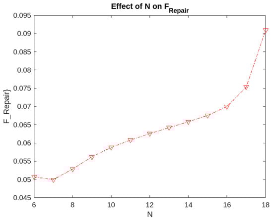
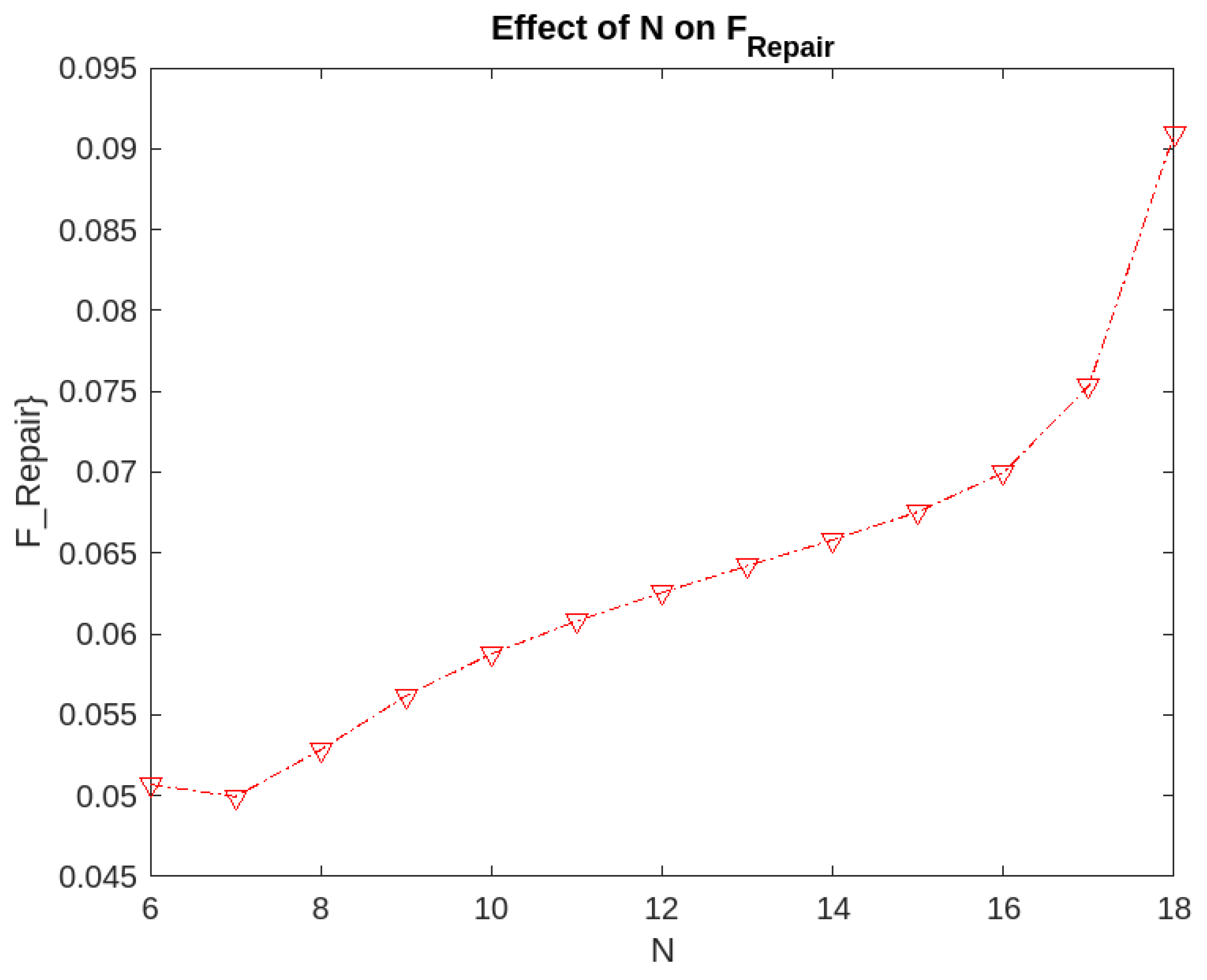
Figure 1.
Effect of parameter N on the fraction of time for which the servers are under repair.
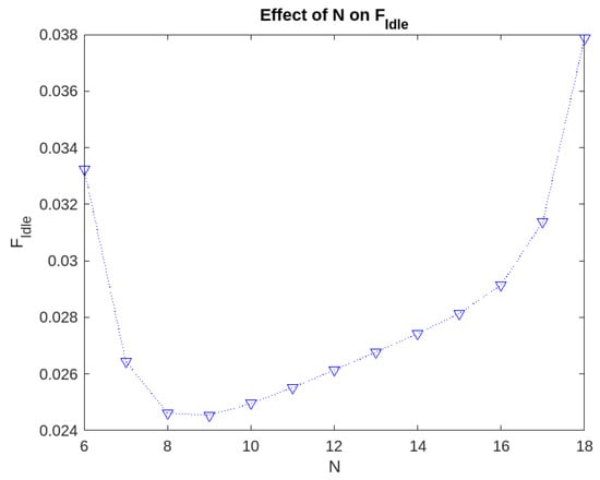
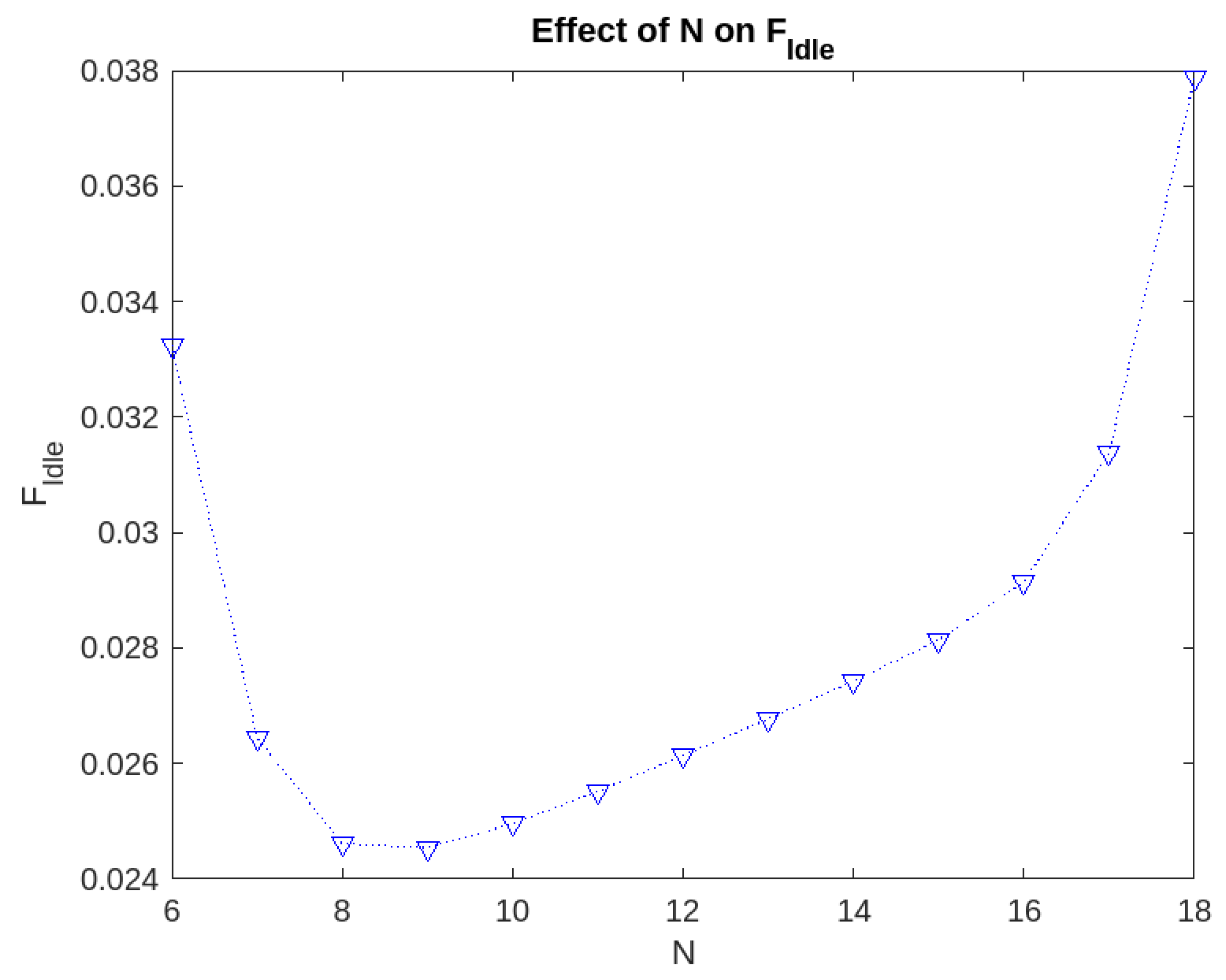
Figure 2.
Effect of the level N on the fraction of time for which the servers are idle.
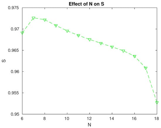
Figure 3.
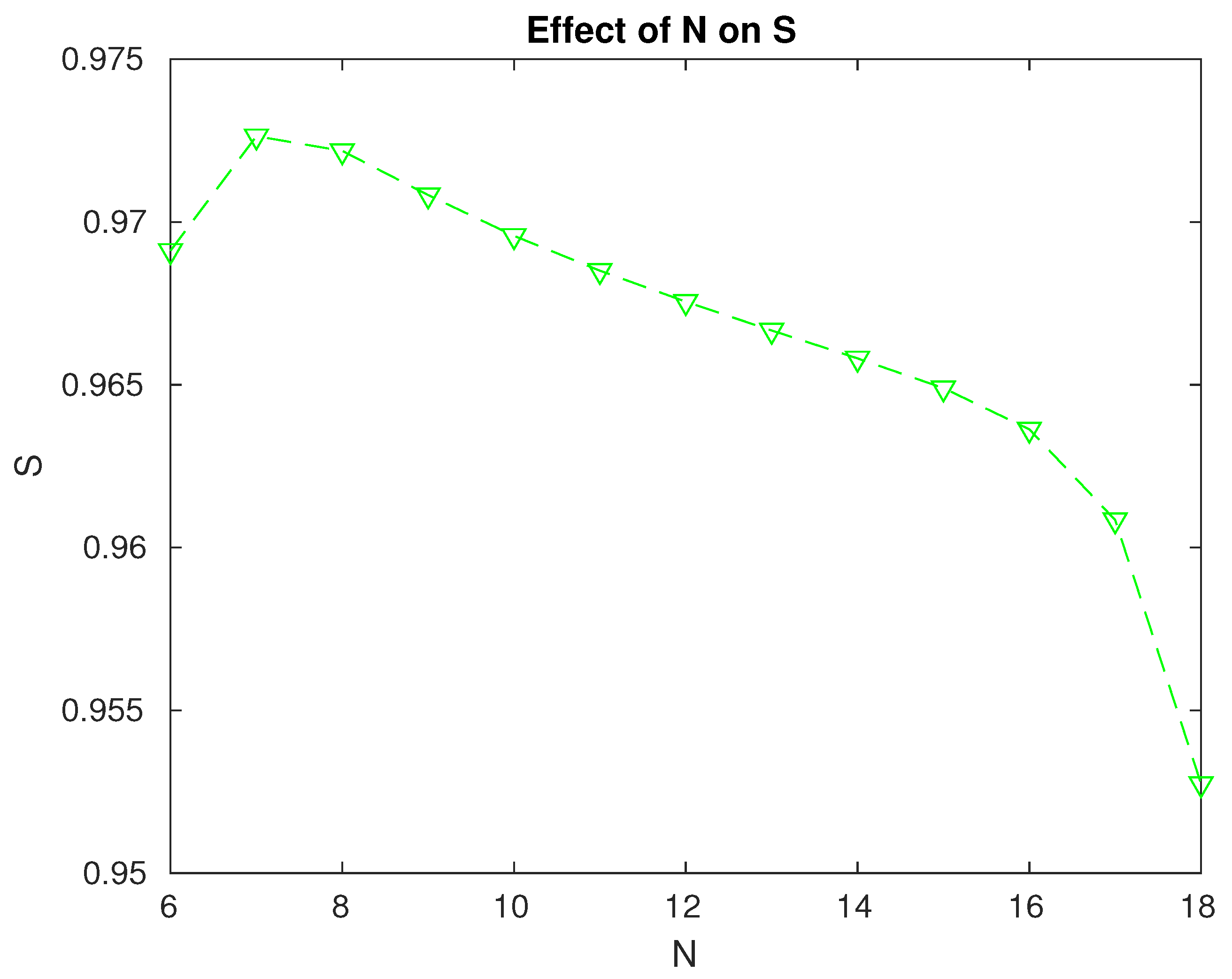
Effect of the level N on the reliability of the system.
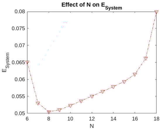
Figure 4.
Effect of the level N on .
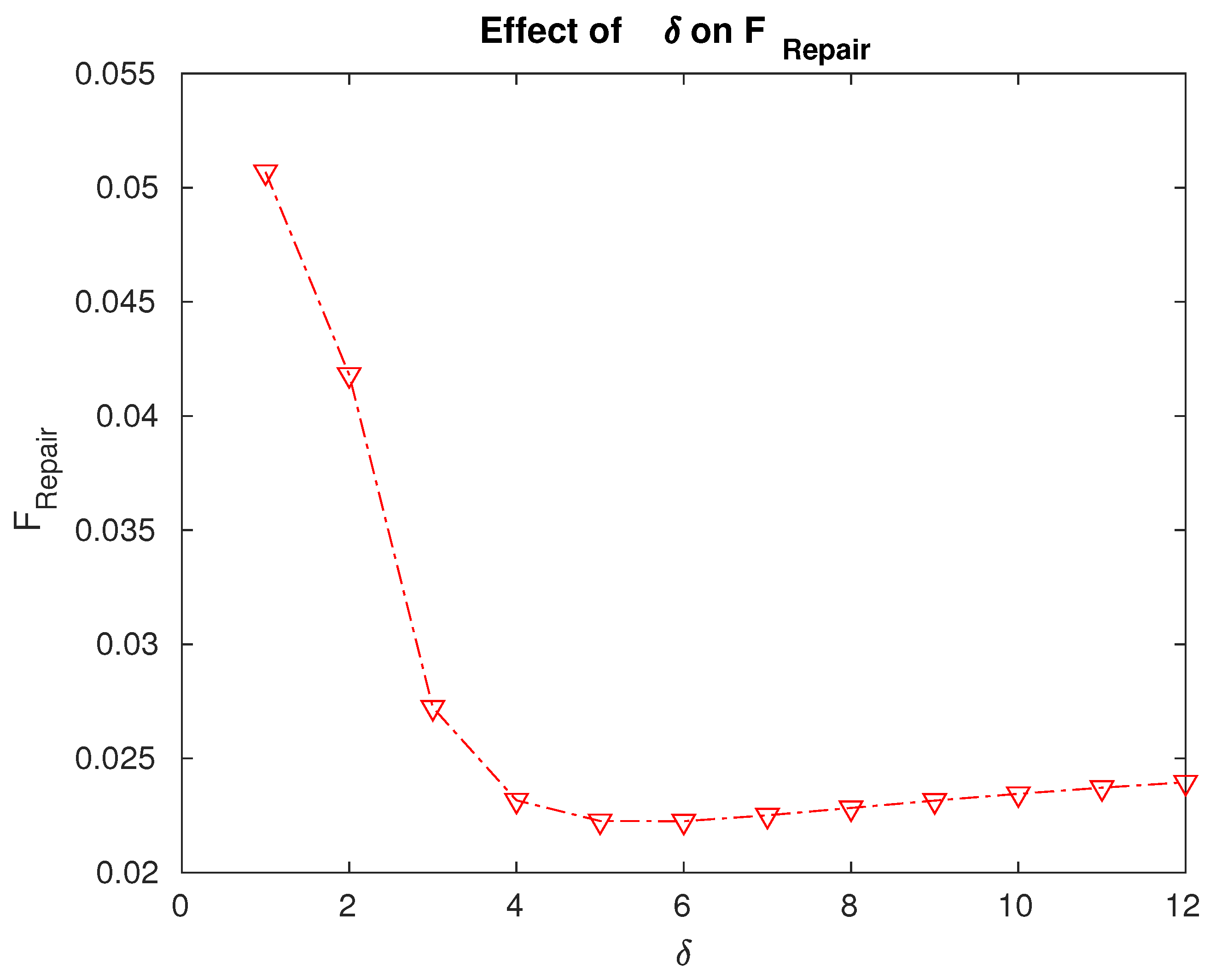
- The fraction of time for which the servers are under repair is the minimum for a value . To minimize , we need to initiate the repair process when the number of non-operational servers is 13.
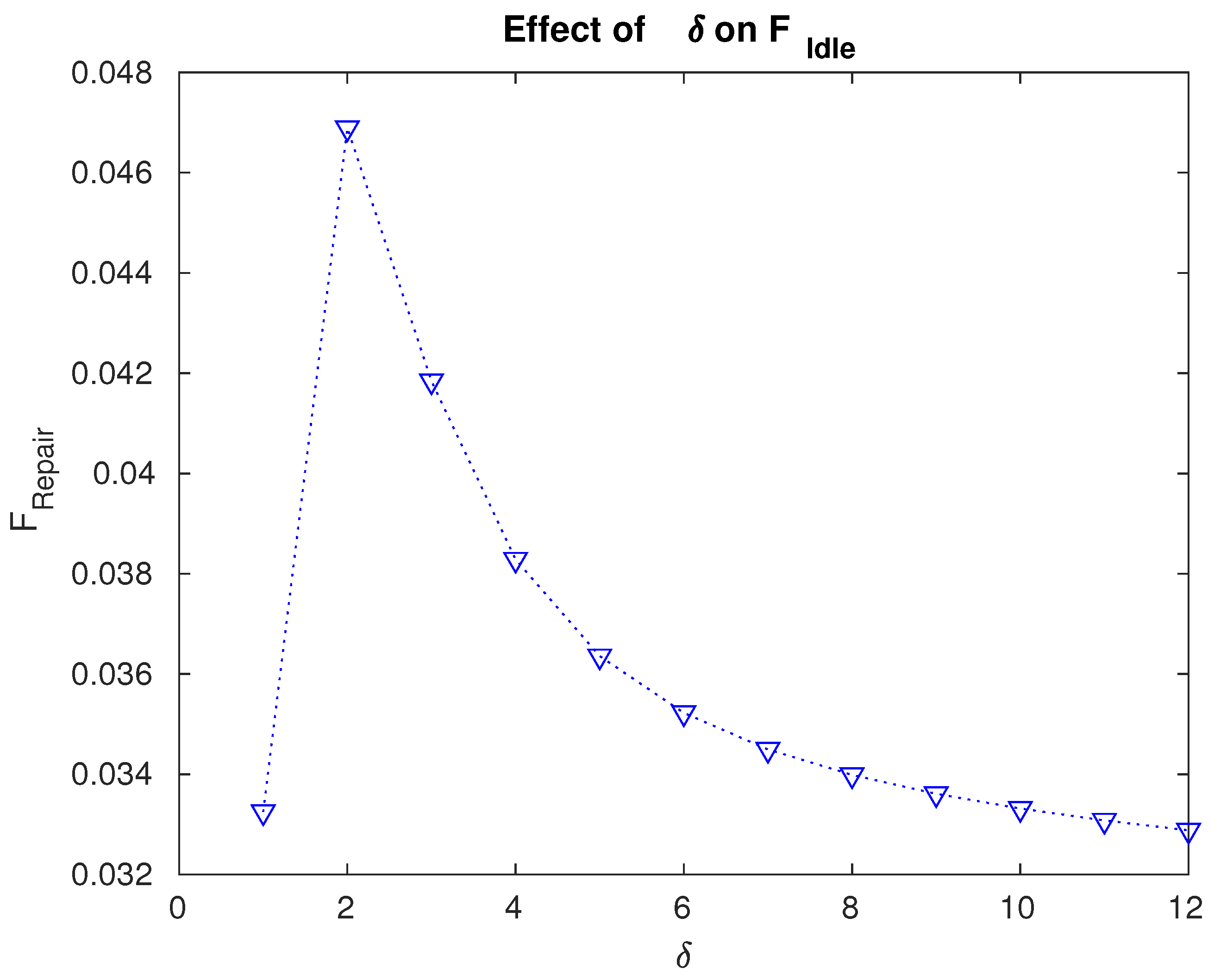
- The fraction of time for which the servers are idle can be minimized if we choose . It plays a crucial role in enhancing the cost-effectiveness of the model.
- The system reliability is maximum when . We can achieve a more reliable system if we take into consideration the results in Figure 3.
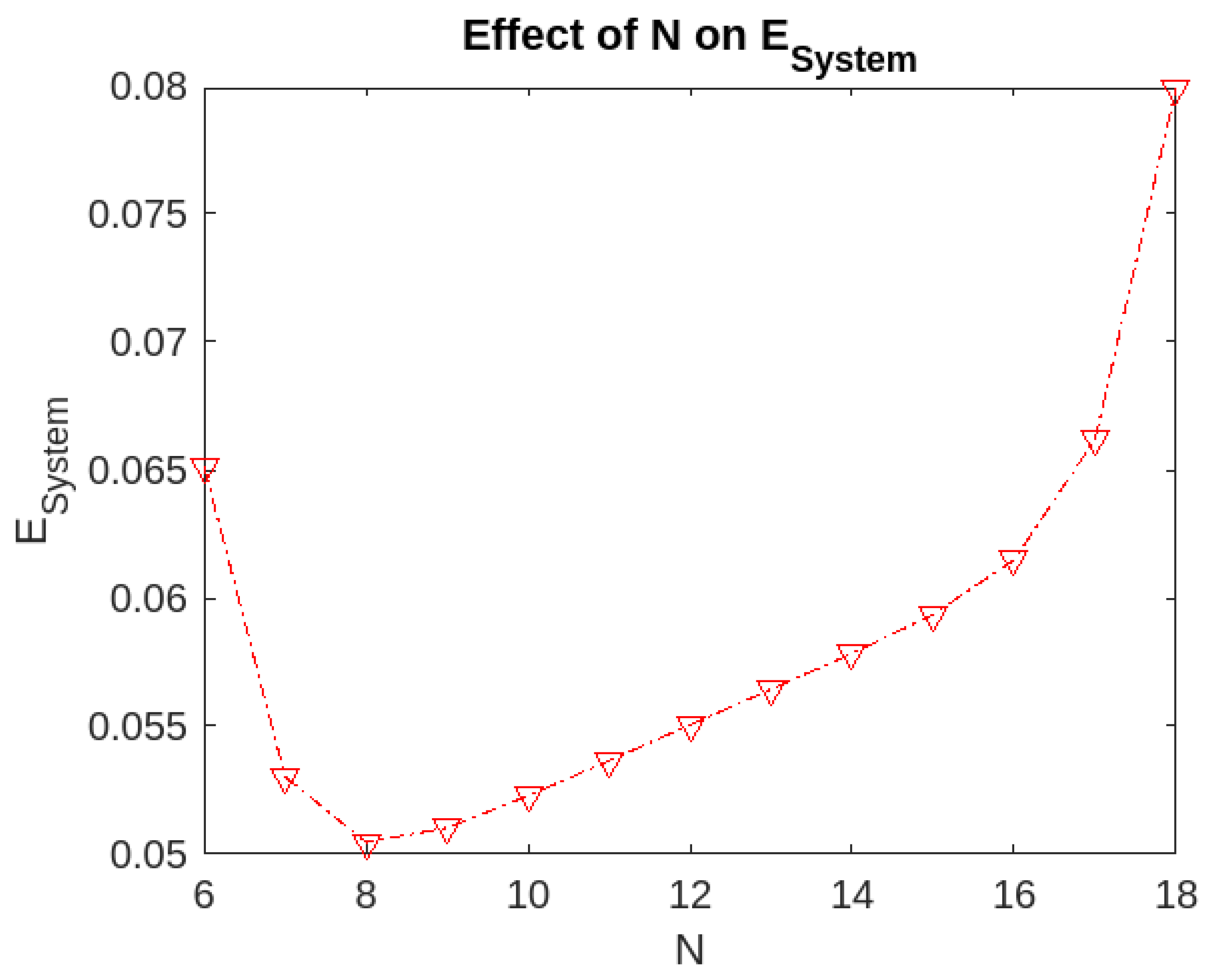
- The expected number of customers found waiting in the system is the minimum if we choose . The value of the expected number of customers is low as the servers are working in parallel.
The above example illustrates that the analysis can guide us in properly managing the repair policy with specific objectives.
6.2. Effect of the Repair Rate on the Performance of the System
In this section, we study the effect of the repair rate on the performance of the system. In this example, the following parameters are kept fixed with values as given below:
Table 2.
Effect of repair rate on , , S and .
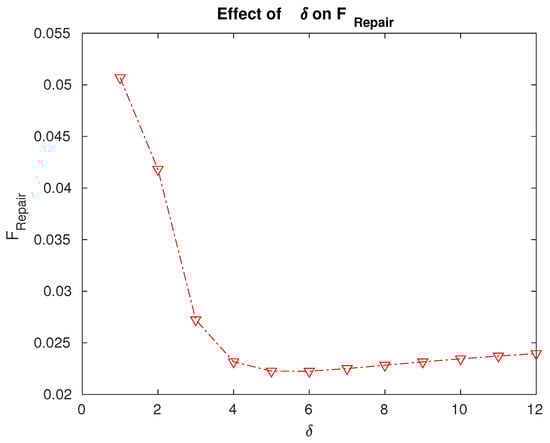
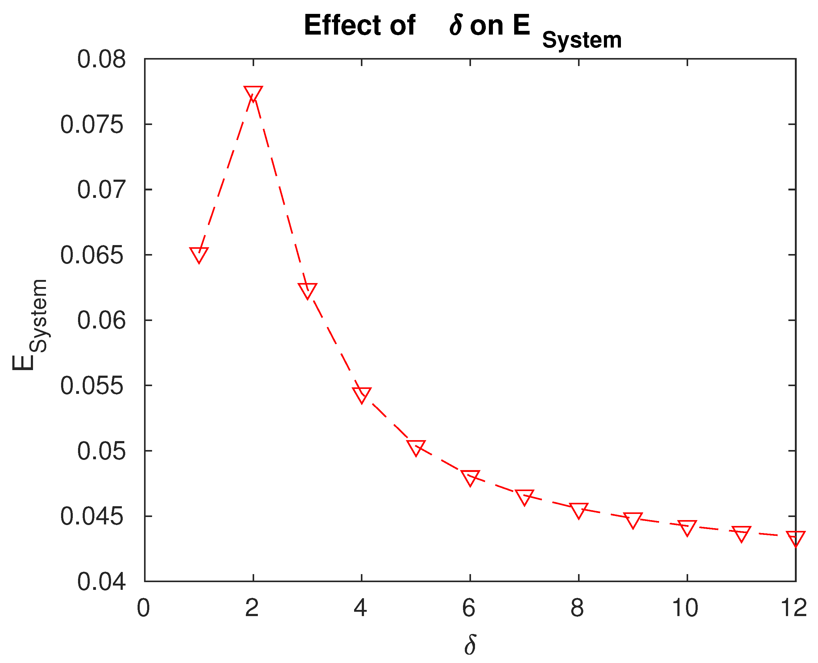
Figure 5.
Effect of the repair rate on the fraction of time for which the servers are under repair.
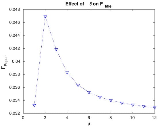
Figure 6.
Effect of the repair rate on the fraction of time for which the servers are idle.
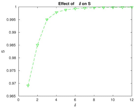
Figure 7.
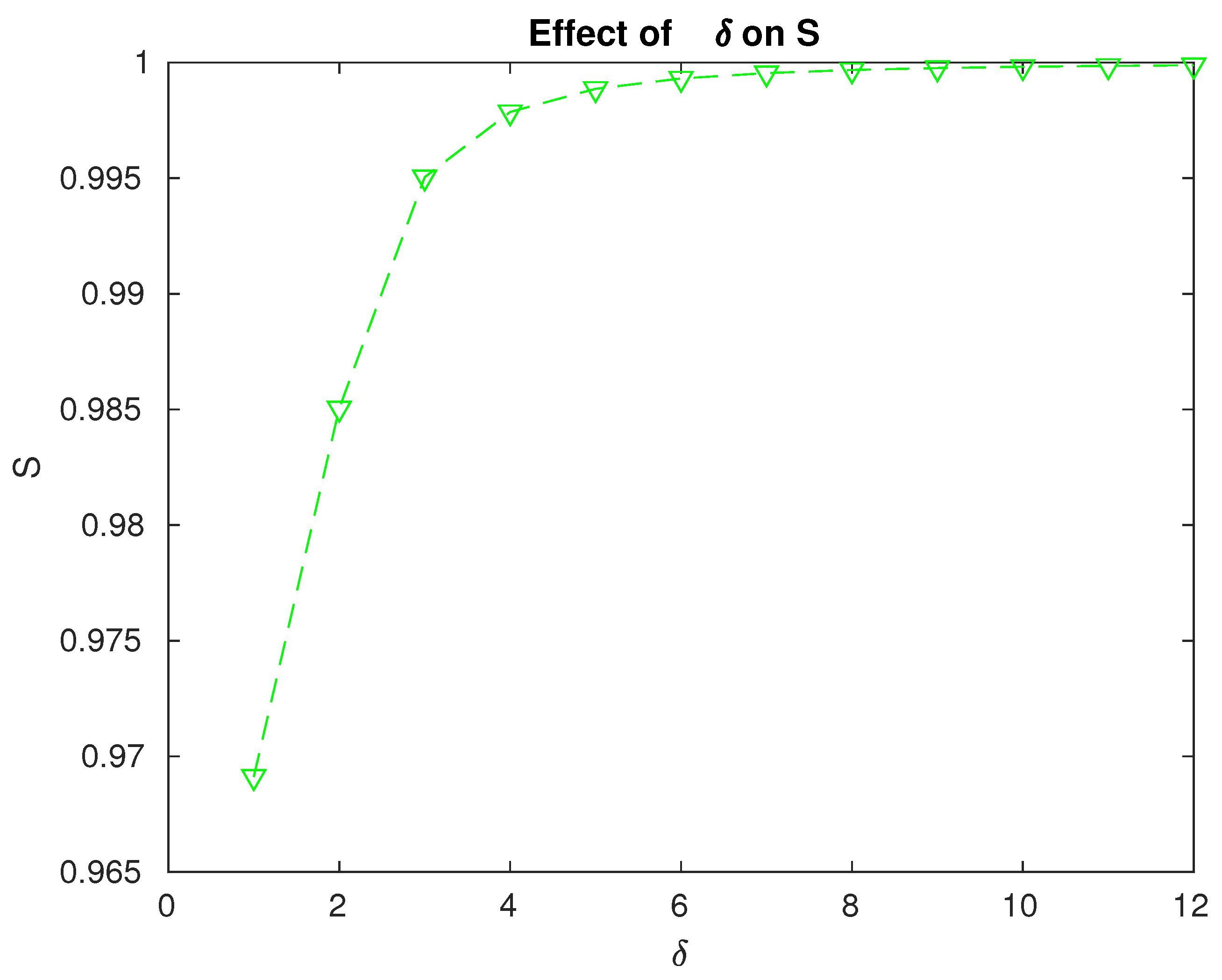
Effect of the repair rate on the reliability of the system.
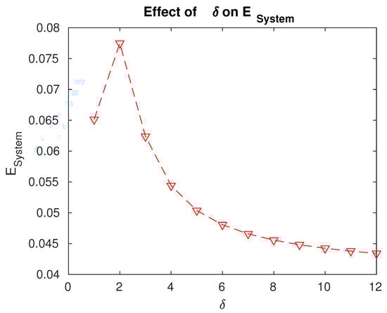
Figure 8.
Effect of on .
- The fraction of time for which the servers are under repair is the minimum for a value . We can decide to what extent we need to enhance the repair facilities or resources based on the data in Figure 5.
- The fraction of time for which the servers are idle is maximum for . The data in Figure 6 play a crucial role in specifically designing the facilities so that the idle time of the servers can be effectively utilized and the entire system can be managed accordingly.
- The system reliability increases with increasing values of as expected. The rate at which this increase occurs helps us to decide on the optimum value to be considered when compared to the resources or efforts involved in enhancing the repair facilities; see Figure 7.
- The expected number of customers found waiting in the system is maximum for .
7. Cost Analysis and Optimization Problem
Cost analysis plays an important role in decision making or in formulating policies related to the working of any system that we encounter in everyday life. In this section, we propose a cost function related to the system under consideration. We consider an optimization problem to find the value of the level N of the N-policy of the repair. With the help of numerical examples as well as graphical illustrations, we show that an optimal value N exists so that the total expected cost is the minimum. We also study the effect of the repair rate on the the total expected cost.
To determine the optimal level of N at which the repair facility can start working and to determine the effectiveness of enhancing the repair rate, we proceed as follows. For the cost analysis, we define the following costs.
- : Establishment cost or setup cost.
- : Holding cost per customer per unit time.
- : Unit time cost to run the repair mechanism.
- : Unit time cost incurred due to the idleness of the servers.
- : unit time revenue received from the busy servers.
- : Unit time revenue received when at least k servers are operational.
The expected total cost is
We fix the following values:
The values of other parameters are the same as in Section 6.
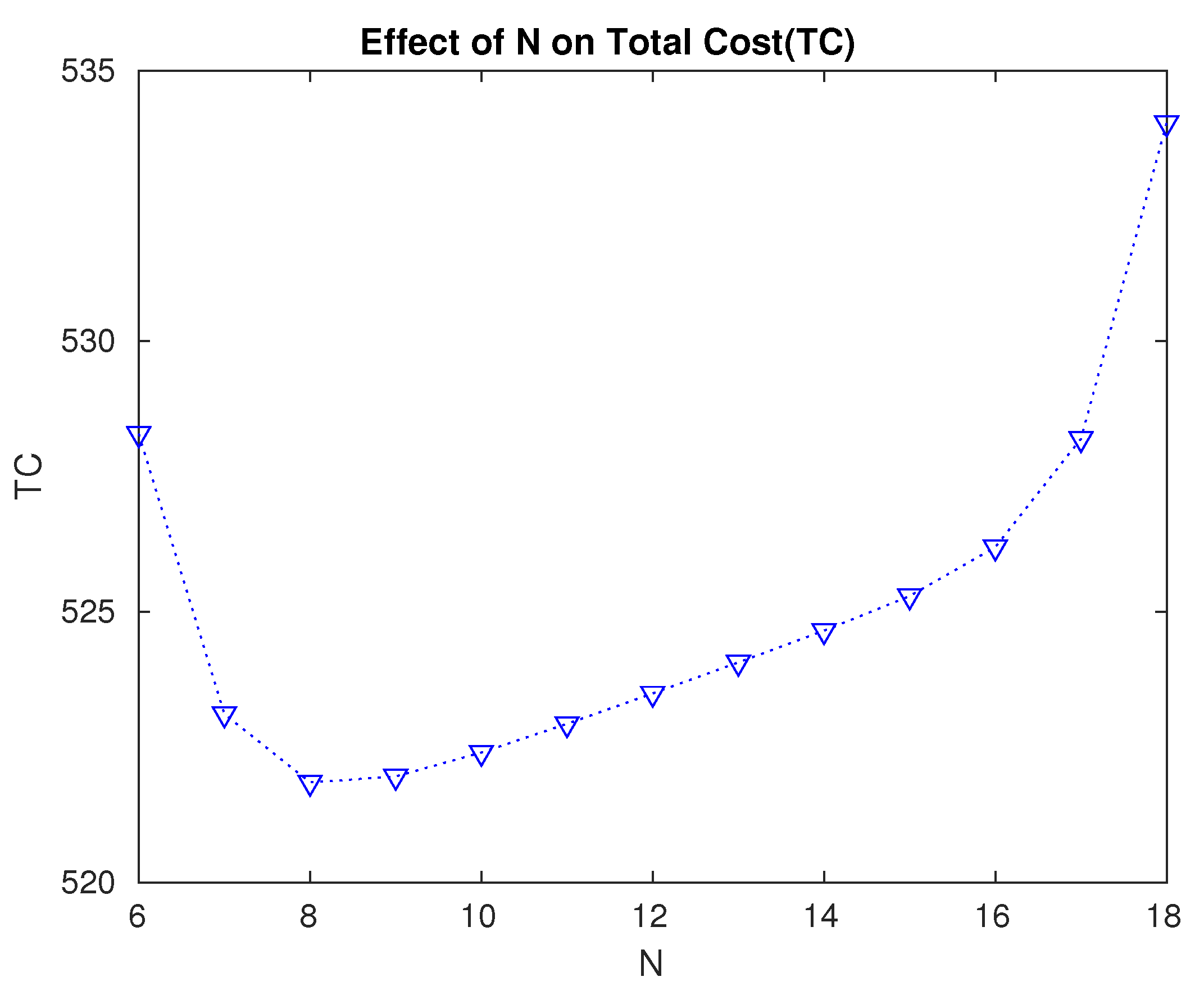
- From Table 3 and Figure 9, we see that the optimal value of the level N is , for which the total expected cost is the minimum. Thus, it is optimal to wait until 12 servers are non-operational before starting the repair.
Table 3. Effect of N and on expected total cost.
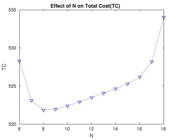 Figure 9. Effect of the changes in level N on the expected total cost.
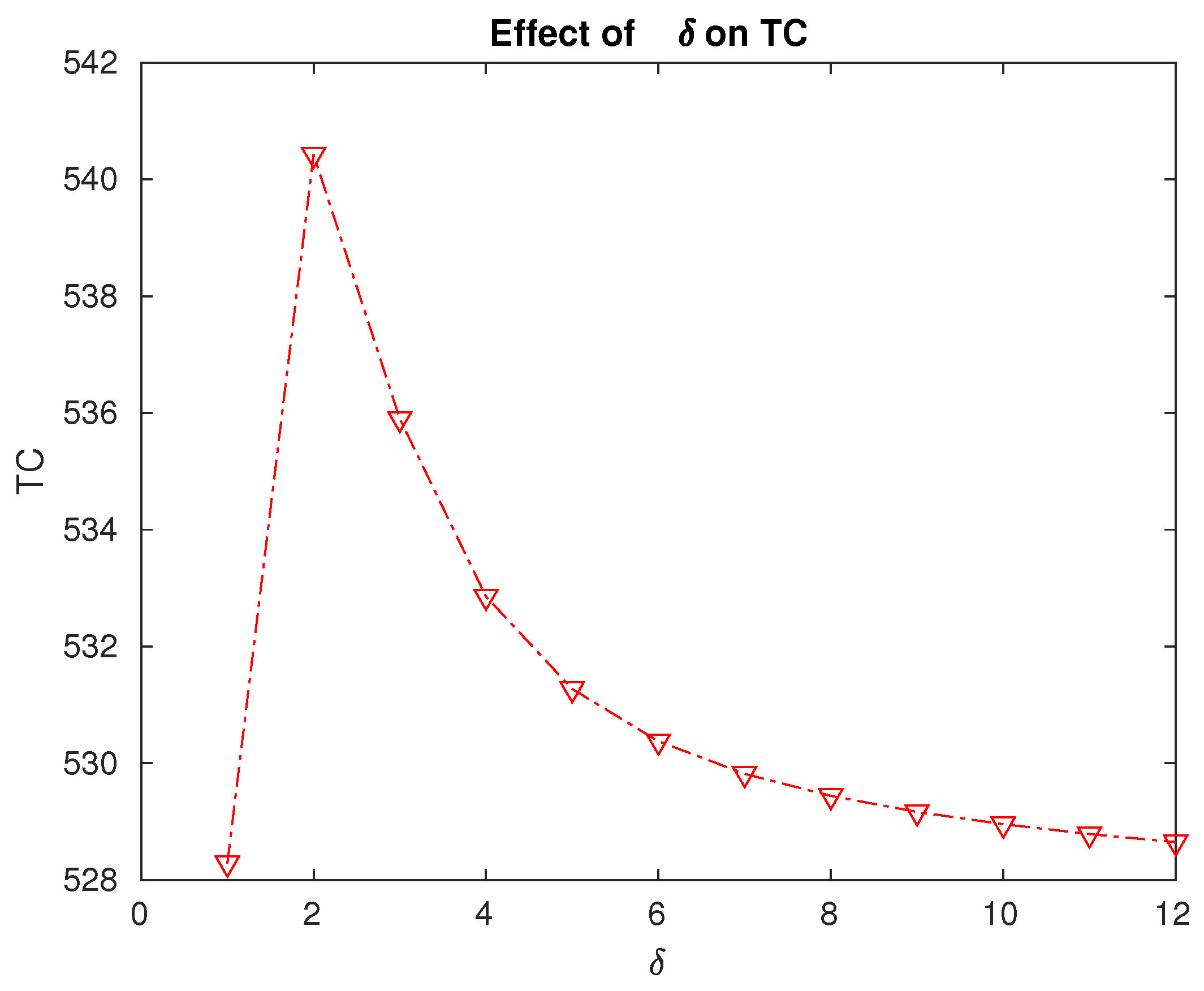
 - From Table 3 and Figure 10, it can be seen that the expected total cost is the maximum when the repair rate is . This means that if we spend more to increase the rate at which the repair is performed from 1 to 2 or more, it will not be reflected in the total expected cost. Thus, a decision regarding the facilities to be arranged to ensure a specific repair rate can be made using this cost analysis. In this specific numerical example, it is enough to ensure a repair rate of at most .
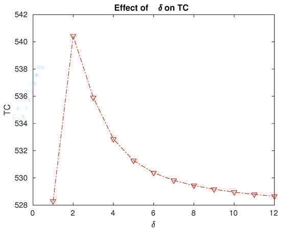 Figure 10. Effect of the repair rate on the expected total cost.
 - By analyzing the problem numerically, we can decide on the optimal values of the level N of the -policy and also the optimal repair rate to be maintained.
8. Conclusions
This paper studies a multi-server queuing system with the N-policy of repair, by viewing it as a k-out-of-n:G system. The steady-state distributions of various system states are computed. The distribution of server idle times is analyzed. Under the assumption of a sufficiently large number of customers in the system, the distribution of the first passage times from an inoperative state to an n server state and vice versa has been found. The assumption of a sufficiently large number of customers in the system is made to avoid complications that may arise due to future arrivals. Other system performance measures such as system reliability, the expected number of failed servers, etc., are computed.
The effect of an increase in the level N and the repair rate on various performance measures, when other parameters are kept fixed, is studied numerically and graphically. An increase in the repair rate significantly increases the system reliability and decreases the expected number of customers in the system. It reduces the idleness of servers and reduces the fraction of time for which the servers are under repair. On the other hand, an increase in N increases the fraction of time for which the servers are under repair. However, as N increases, the idleness of servers and the expected number in the system first decrease and then increase, while the system reliability first increases and then decreases. The optimal value of N depends on the parameters of the system. The examples illustrate how an optimal policy could be derived for a multi-server queuing system, keeping in mind certain specific objectives. A cost function has been constructed and the results of the cost analysis are presented.
There can be several extensions to the problem considered in this paper. An extension of the present work to one in which consecutive k-out-of-n systems provide a service to customers, either linearly or in a circular fashion, is proposed for future research. A similar study of the k-out-of- system is underway. Moreover, the k-out-of-n system could be analyzed under both HOT and WARM conditions.
Author Contributions
Conceptualization, A.K.; Methodology, A.N.J.; Validation, A.P.M.; Formal analysis, A.N.J.; Data curation, A.P.M.; Writing—original draft, A.K., A.N.J. and A.P.M.; Writing—review & editing, A.K., A.N.J. and A.P.M.; Supervision, A.K. All authors have read and agreed to the published version of the manuscript.
Funding
Dr. Anu Nuthan Joshua and Dr. Ambily P. Mathew received support from DST-RSF research project number 22-49-02023 (RSF) and research project number 64800 (DST) for the preparation of this publication. https://search.crossref.org/funding.
Data Availability Statement
Data are contained within the article.
Conflicts of Interest
The authors declare no conflicts of interest.
Notations and Abbreviations
The following abbreviations are used in this manuscript:
| Continuous-time Markov chain | |
| process | Quasi-birth–death process |
| e | All one vector with appropriate dimension |
| Identity matrix of order | |
| Square matrix of appropriate size with all zero entries except the entries , which are equal to 1 | |
| Square matrix of appropriate size with all zero entries except the entries , which are equal to 1 | |
| Matrix of appropriate size with all zero entries except the entry , which is equal to 1 | |
| Column vector of appropriate dimension with all zero entries except the entry i, which is equal to 1 | |
| Transpose of matrix A | |
| Matrix whose entries are 0, of appropriate size | |
| Kronecker product; if is a matrix of order and if B is a matrix of order , then will denote a matrix of order |
References
- Barlow, R.E.; Proschan, F. Mathematical Theory of Reliability; John Wiley and Sons: New York, NY, USA, 1965. [Google Scholar]
- Krishnamoorthy, A.; Sathian, M.K.; Narayanan Viswanath, C. Reliability of a k-out-of-n System with Repair by a Single Server Extending Service to External Customers with Pre-emption. Electron. J. Reliab. Theory Appl. 2016, 11, 61–93. [Google Scholar]
- Yadin, M.; Naor, P. Queueing system with a removable service station. Oper. Res. Q. 1963, 14, 393–405. [Google Scholar] [CrossRef]
- Krishnamoorthy, A.; Ushakumari, P.V.; Lakshmy, B. k-out-of-n-system with repair: The N-policy. Asia-Pac. J. Oper. Res. 2002, 19, 47–61. [Google Scholar]
- Yen, T.-C.; Wang, K.-H.; Chen, J.-Y. Optimization Analysis of the N-Policy M/G/1 Queue with Working Breakdowns. Symmetry 2020, 12, 583. [Google Scholar] [CrossRef]
- Vemuri, V.K.; Boppana, V.S.N.H.P.; Kotagiri, C.; Bethapudi, R.T. Optimal strategy analysis of an N-policy two-phase MX/M/1 queueing system with server startup and breakdowns. Opsearch 2011, 48, 109–122. [Google Scholar] [CrossRef]
- Singh, C.J.; Jain, M.; Kumar, B. Analysis of queue with two phases of service and m phases of repair for server breakdown under N-policy. Int. J. Serv. Oper. Manag. 2013, 16, 373–406. [Google Scholar] [CrossRef]
- Neuts, M.F. Matrix—Geometric Solutions in Stochastic Models: An Algorithmic Approach; The Johns Hopkins University Press: Baltimore, MD, USA, 1981. [Google Scholar]
- Gross, D.; Harris, C. Fundamentals of Queuing Theory, 3rd ed.; John Wiley: Chichester, UK, 1988. [Google Scholar]
Disclaimer/Publisher’s Note: The statements, opinions and data contained in all publications are solely those of the individual author(s) and contributor(s) and not of MDPI and/or the editor(s). MDPI and/or the editor(s) disclaim responsibility for any injury to people or property resulting from any ideas, methods, instructions or products referred to in the content. |
© 2024 by the authors. Licensee MDPI, Basel, Switzerland. This article is an open access article distributed under the terms and conditions of the Creative Commons Attribution (CC BY) license (https://creativecommons.org/licenses/by/4.0/).