Dynamic Convolution Neural Networks with Both Global and Local Attention for Image Classification

Abstract

Convolution is a crucial component of convolution neural networks (CNNs). However, the standard static convolution has two primary defects: data independence and the weak ability to integrate global and local features. This paper proposes a novel and efficient dynamic convolution method with global and local attention to address these issues. A building block called the Global and Local Attention Unit (GLAU) is designed, in which a weighted fusion of global channel attention kernels and local spatial attention kernels generates the proposed dynamic convolution kernels. The GLAU is data-dependent and has better adaptability and the ability to integrate global and local features into each layer. We refer to such modified CNNs with GLAUs as “GLAUNets”. Extensive evaluation experiments for image classification compared to classical CNNs and the state-of-the-art dynamic convolution neural networks were conducted on the popular benchmark datasets. In terms of classification accuracy, the number of parameters, and computational complexity, the experimental results demonstrate the outstanding performance of GLAUNets.

1. Introduction

In the past decade, convolution neural networks (CNNs) have become a powerful tool in various visual problems [1,2,3,4,5,6,7] and attracted considerable attention. In CNNs, convolution plays a crucial role in capturing helpful information. CNNs rely on stacking multiple convolution layers and using various convolution kernels to extract essential features in each layer. It is well known that the standard convolution kernel of each layer has a good local feature extraction ability. However, the standard convolution has two primary defects: data-independence and a weak ability to integrate global and local information in each layer. Firstly, the standard convolution is independent of the input data, which means that the convolution kernel is fixed regardless of different input data. Consequently, this lack of data awareness will lead to suboptimal extraction of features, especially when the input data have complex relationships or patterns that cannot be captured using the same kernel. Secondly, the standard convolution is good at extracting local features, but capturing global representation in each layer is difficult. By stacking multiple convolution layers, CNNs have the ability not only to extract multiscale local features but also compose them to construct highly abstract representations. However, stacking many convolution layers can make it challenging to form connections between the long-distance features, resulting in increased computational demands and difficulty in optimization. Therefore, the problem of the weak ability to integrate global and local features is more prominent. This will lead to a limit on the amount of global information used for image classification. Dynamic convolution methods have been proposed to adaptively generate convolution kernels based on data contents to change the data-independent nature of standard convolution. Several researchers [8,9,10,11,12,13,14] provided a foundation for the development and application of dynamic convolution in computer vision and related fields. They demonstrated the potential of dynamic convolution to adapt to different inputs and improve the accuracy and efficiency of CNNs. However, dynamic convolutions improve adaptability; the kernel generated by most methods only adapts to the spatial locations or channel domain. Otherwise, existing fully adaptive methods will dramatically increase parameters and make them less effective. To address the limitation of local and global information integration, researchers have proposed using other types of pooling layers [15], convolution layers [16], and skip connections [17] that are designed to capture information from different regions and scales of the input data. However, the above methods still need to significantly improve the ability to integrate global and local information in each layer after stacking multiple convolution layers.

In this work, we present a building block called the GLAU. Specifically, a GLAU is a weighted fusion module of two attention branches. One attention branch is designed to generate the local spatial attention convolution kernel dynamically, and the other is used to generate the global channel attention convolution kernel dynamically. A weighted fusion module merges these two branches to generate the final convolution kernels of GLAUs. Moreover, the weights in the fusion module are obtained from the parameters that the network training can learn. Because our kernels are dynamically generated based on local and global input data information, our method is data-dependent and can better integrate global and local features in each layer. Our key contributions are summarized as follows:

• Integrating global and local features in each layer. We propose a novel and efficient dynamic convolution method with both global and local attention through GLAUs. In each layer, our dynamic convolution makes full use of the statistical information of the feature map to integrate global and local features, which greatly improves the discrimination ability of feature representation and the performance of image classification.
• Dynamic convolution kernels (spatially specific and channel-specific). A weighted fusion of global channel and local spatial attention kernels generates the proposed dynamic convolution kernels. The generated convolution kernels are distinct in terms of spatial location and channel position; that is to say, the proposed dynamic convolution is spatially specific and channel-specific and has better adaptability, resulting in more efficient and accurate feature representation. Notably, although the proposed dynamic convolution is spatially specific and channel-specific, our parameter quantity is rather tiny.
• Outstanding performance of GLAUNets. We evaluate the proposed GLAUNets on classic image classification datasets, CIFAR-10, CIFAR-100, and Mini-ImageNet compared with baseline methods and the state-of-the-art dynamic convolution networks. Extensive experiments demonstrate the outstanding performance of GLAUNets.

2. Related Works

2.1. Deep Convolution Neural Networks

Deep convolution neural networks (DCNNs) play a crucial role in computer vision due to their powerful feature extraction capabilities. In particular, since AlexNet [1] won the ImageNet competition, DCNNs have become popular. The classic DCNNs enable the network to be continuously improved for better performance, such as ResNet [17], VGG [18], GoogLeNet [19], and DenseNet [20]. Over the years, many researchers have studied DCNNs from different aspects. One common approach is to increase the depth of the network, as demonstrated in [1,17,18].

Several studies [19,21,22] have demonstrated that increasing the width of the network can enhance model performance. Moreover, a recent study [23] demonstrated that increasing cardinality is more effective than adjusting the depth and width while maintaining comparable complexity.

ConvNeXt [24] has shown performance comparable to that of the latest vision transformers [25,26]. Although existing DCNNs have paved the way for more profound and more powerful networks, they have also revealed some drawbacks. Specifically, the fixed and local nature of traditional static convolution kernels in each convolutional layer limits the network’s ability to adapt and capture global representations, thereby increasing computational overhead in deeper networks. To address these limitations, the proposed GLAU introduces a novel general-purpose architecture that dynamically generates convolution kernels by integrating global and local information from input data, thereby reducing computational complexity while preserving performance.

2.2. Attention Mechanism

The attention mechanism originated from the study of human vision. Various attention mechanisms [27,28,29,30,31] have been developed and significantly impacted the field of computer vision. Incorporating attention mechanisms into deep learning has enhanced the performance of various models in recent years. The attention mechanism enables flexible application to various neural network structures, enhancing performance by emphasizing crucial features and suppressing irrelevant ones. Context Encoders [32] is a proposed attention model capable of automatically learning image content descriptions, thus introducing the attention mechanism to the field of image processing and leading to a paradigm shift. The STN [33] indicates that different regions in an image contribute differently to a task. Therefore, a spatial transformer module is proposed to allow the convolution neural networks to map the differences. The renowned attention network SENet [34] models channel interdependencies through a squeeze-and-excitation block operation, thereby reducing network error rates. For CBAM [35], it was pointed out that the convolution operation mixes channel features with spatial features in the feature extraction process, leading to developing a two-branch attention method combining channel and spatial attention. The coordinate attention (CA) [36] factorizes channel attention into two 1D feature encoding processes that aggregate features along the two spatial directions. Inspired by these works, the attention mechanism has experienced rapid development, with researchers proposing various methods such as SKNet [37], ECANet [38], and DCANet [39]. This study focuses on integrating global and local information from input features, proposing a novel and efficient dynamic convolution method with global and local attention.

2.3. Dynamic Convolution

Several works [9,10,11] tried to linearly combine traditional convolution kernels by learning a set of coefficients. Deformable convolution [40] is designed to learn to adapt kernel points to local geometry. Additionally, some unique structures have been devised to further substantiate the role of dynamic convolution. For instance, SKNet [37] convolves feature maps at multiple scales via three operators, “Split-Fuse-Select”, and then merges the resulting features to generate the convolution kernel dynamically. TVConv [41] uses affinity maps and a weight-generating block to adapt to layout-specific tasks. Some studies [11,42] dynamically generated convolution kernels based on the input feature map. DFN [8], Hyper Networks [43], and Involution [44] work from the perspective of dynamic parameters and produce network parameters to accommodate different inputs. Numerous studies [45,46,47,48,49,50] have demonstrated that dynamic convolution has significant potential to enhance the performance of DCNNs, thus attracting comprehensive attention. KernelWarehouse [13] redefines the basic concepts of “kernels” and “assembling kernels” in dynamic convolution and enhances the dependencies of convolution parameters within the same layer and between successive layers through tactful kernel partition and warehouse sharing.

The goal of dynamic convolution is to balance network performance with computational load. Conventional approaches to improving network performance (wider and deeper) tend to result in higher computing costs and are therefore not friendly to efficient networks. In this work, the following six classical dynamic convolution methods are used as a comparison. Among them, DyConv [10] and CondConv [9] were developed in the same period, and the concept of dynamic convolution correlation was proposed. DyConv uses the SE attention mechanism to assign attention weights to the convolutional kernel, which can be easily embedded to replace the convolution of the existing network architecture. CondConv is equivalent to a linear combination of multiple static convolutions which is more efficient in calculations. Subsequently, DCD [51] revisited dynamic convolution from the perspective of matrix factorization, which is more interpretable and more accessible to train. For DDF [42], decoupling the generation of convolutional kernels into spatial and channel convolutional kernels is proposed. Involution [44] establishes the association between dynamic generation and the attention mechanism and analyzes the opposite characteristics of convolution and involution. OdConv [52] can be regarded as a continuation of CondConv, which extends the dynamic characteristics of one dimension in CondConv and, at the same time, considers the dynamics of the space, input channel, output channel, and other dimensions while adopting a multi-dimensional attention mechanism to learn complementary attention along the four dimensions of the kernel space through the parallel strategy.

Among them, we observed that the less the generated convolution kernel is shared, the better its performance, albeit at the expense of a considerably increased parameter count. To reduce the parameters, these methods have no choice but to share convolution kernels in the channel domain. The typical representation is Involution. Based on this observation and analysis, we consider the unshared convolution kernel. The proposed GLAU’s convolution kernel is spatially specific and channel-specific, meaning each spatial and channel position of the input feature has its convolution kernel. The GLAU must maintain accuracy with fewer parameters. Currently, further research is needed in this area.

3. Global and Local Attention Unit

This section begins with an overview of our GLAU approach (Section 3.1). We then describe the form of our GLAU, clarify its nature, and detail its implementation with a global module (Section 3.2), a local module (Section 3.3), a fusion module (Section 3.4), and computational complexity (Section 3.5).

3.1. Overview of GLAUs

An image’s global and local information is crucial to portraying an image. Our fundamental motivation was to decouple the convolutional kernel’s generation process into two branches: one to describe the global information and the other to describe the local information. Formally, the GLAU is decoupled. However, in essence, in the global channel attention module, for each feature map, the mean and standard deviation are calculated in three directions along the spatial dimension, which fully considers the acquisition of local information. In the local spatial attention module, along the channel dimension, the mean and standard deviation are also calculated for each feature map, and the acquisition of global information is also fully considered. Second, for the feature maps generated by the two branches, the feature fusion is carried out through an efficient fusion module to obtain a better convolution kernel. Therefore, the GLAU’s ability to integrate global and local features is justified.

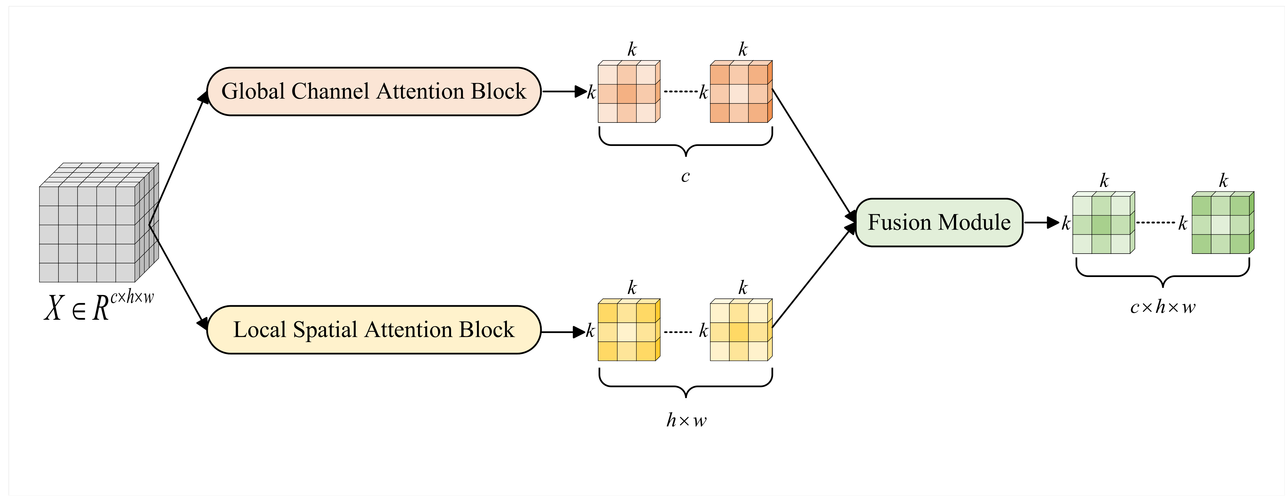
We propose a dynamic convolution method incorporating both global and local attention. We have devised a building block termed the Global and Local Attention Unit (GLAU). The GLAU can adaptively generate convolution kernels through a weighted fusion of global channel attention kernels and local spatial attention kernels. The detailed structure of the GLAU is illustrated in Figure 1. We denote $X\in R^{c\times h\times w}$ as an input instance of the GLAU. The GLAU is designed to contain two branches and a fusion module. One of these branches is the global channel attention branch, and the other is the local spatial attention branch. The fusion module utilizes learnable parameters to integrate the two branches above.

3.2. Global Channel Attention Block

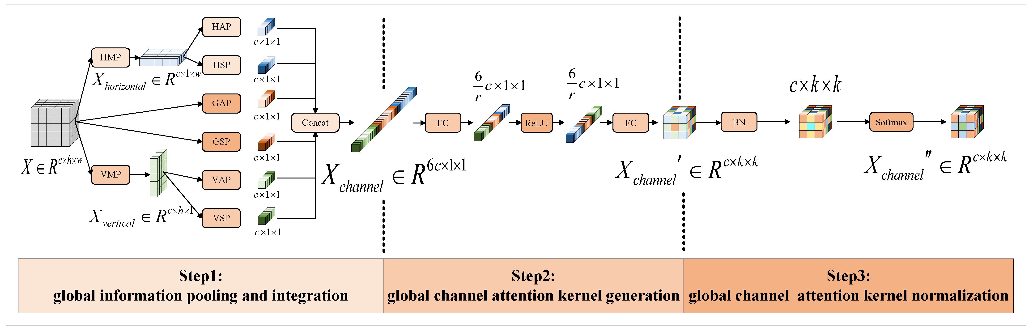
In the channel branch, we aim to find a global feature that accurately describes the global information of X. Instead of utilizing global average pooling, we employed two statistics—the mean and standard deviation—in three directions (horizontal, vertical, and spatial) to extract comprehensive global features. The process of deriving the global channel attention kernels consists of three steps: global information pooling and integration, generation of global channel attention kernels, and normalization of global channel attention kernels. Global information pooling and integration for extracting an intermediate global information representation is expressed as $X_{channel}\in R^{(d\times c)\times 1\times 1}$ from X, where d is the number of global features; global channel attention kernel generation is for generating kernel ${X_{channel}}^{\prime }\in R^{c\times k\times k}$ from $X_{channel}$; and the global channel attention kernel normalization operation consists of a batch normalization (BN) layer, where the BN layer is used to absorb the bias term produced by the fusion of the mean and standard deviation, and a softmax activation function, which converts the original channel attention weights ${X_{channel}}^{″}\in R^{c\times k\times k}$ from ${X_{channel}}^{\prime }\in R^{c\times k\times k}$ into probability distributions for the weighted combination of channels.

The detailed structure of the global channel attention block is illustrated in Figure 2.

First of all, global information pooling and integration refers to the average pooling (AP) and standard deviation pooling (SP) of the feature map $X\in R^{c\times h\times w}$. Global average pooling (GAP) and global standard deviation pooling (GSP) can be calculated using the following equations:

$${\mu }_c=\frac{1}{HW}\sum _{h=1}^H\sum _{w=1}^W{x}_{chw},$$

(1)

$${\sigma }_c=\sqrt{\frac{1}{HW}\sum _{h=1}^H\sum _{w=1}^W{(x_{chw}-{\mu }_c)}^2}.$$

(2)

Then, the two global statistics ${\mu }_{global}\in R^{c\times 1\times 1}$ and ${\sigma }_{global}\in R^{c\times 1\times 1}$ are obtained. Before computing the horizontal and vertical statistics, maximum values are taken in the horizontal and vertical directions to ensure the extraction of the most significant features. We denote the operation that takes the maximum value as the horizontal maximum pooling (HMP) and vertical maximum pooling (VMP), and then the results of applying HMP and VMP to $X\in R^{c\times h\times w}$ are denoted as $X_{\mathrm{horizontal}}\in R^{c\times 1\times w}$ and $X_{\mathrm{vertical}}\in R^{c\times h\times 1}$. Similar to GAP and GSP, with Equations (1) and (2), we can perform horizontal average pooling (HAP), horizontal standard deviation pooling (HSP), vertical average pooling (VAP), and vertical standard deviation pooling (VSP) for $X_{\mathrm{horizontal}}$ and $X_{\mathrm{vertical}}$. Thus, the four direction-aware statistics ${\mu }_{\mathrm{horizontal}}$, ${\sigma }_{\mathrm{horizontal}}$, ${\mu }_{\mathrm{vertical}}$, and ${\sigma }_{\mathrm{vertical}}$ are obtained. The concatenation of the six global statistics $\left(d=6\right)$ along the channel dimension represents global information integration and the pooling output. Intermediate global information representations $X_{channel}\in R^{(d\times c)\times 1\times 1}$ are calculated as follows:

$$X_{\mathrm{channel}}=\left[{\mu }_{\mathrm{global}},{\mu }_{\mathrm{horizontal}},{\mu }_{\mathrm{vertical}},{\sigma }_{\mathrm{global}},{\sigma }_{\mathrm{horizontal}},{\sigma }_{\mathrm{vertical}}\right]$$

(3)

Secondly, we aimed to convert the comprehensive global information representation $X_{channel}$ into global channel attention kernels ${X_{channel}}^{\prime }$. To accomplish this, we utilized two fully connected (FC) layers with a ReLU activation function sandwiched between them, effectively reducing the number of parameters while maximizing the utilization of global information for enhanced model expressiveness. Formally, the calculation of the global channel attention kernel ${X_{channel}}^{\prime }\in R^{c\times k\times k}$ is as follows:

$${X_{channel}}^{\prime }=W_2\left(\delta \left(W_1\left(X_{channel}\right)\right)\right),$$

(4)

where $W_1\in R^{6c\times \frac{6c}{r}}$, $W_2\in R^{\frac{6c}{r}\times (c\times k\times k)}$, and $\delta$ is ReLU activation function.

Thirdly, the global channel attention weights are supposed to model the importance of the global information associated with individual channels to emphasize or suppress them accordingly. To achieve this, the global channel attention kernel ${X_{channel}}^{\prime }\in R^{c\times k\times k}$ becomes a probability distribution for the weighted combination of channels ${X_{channel}}^{″}\in R^{c\times k\times k}$ after a simple combination of the BN layer and the softmax activation function. The BN layer following the two fully connected layers accelerates training. It absorbs bias terms, while the sigmoid activation function acts as a gating mechanism, transforming the weighted channel combination into a probability distribution. Formally, the global channel attention kernel ${X_{channel}}^{\prime }\in R^{c\times k\times k}$ is calculated as follows:

$${X_{channel}}^{″}=Softmax\left(BN\left({X_{channel}}^{\prime }\right)\right).$$

(5)

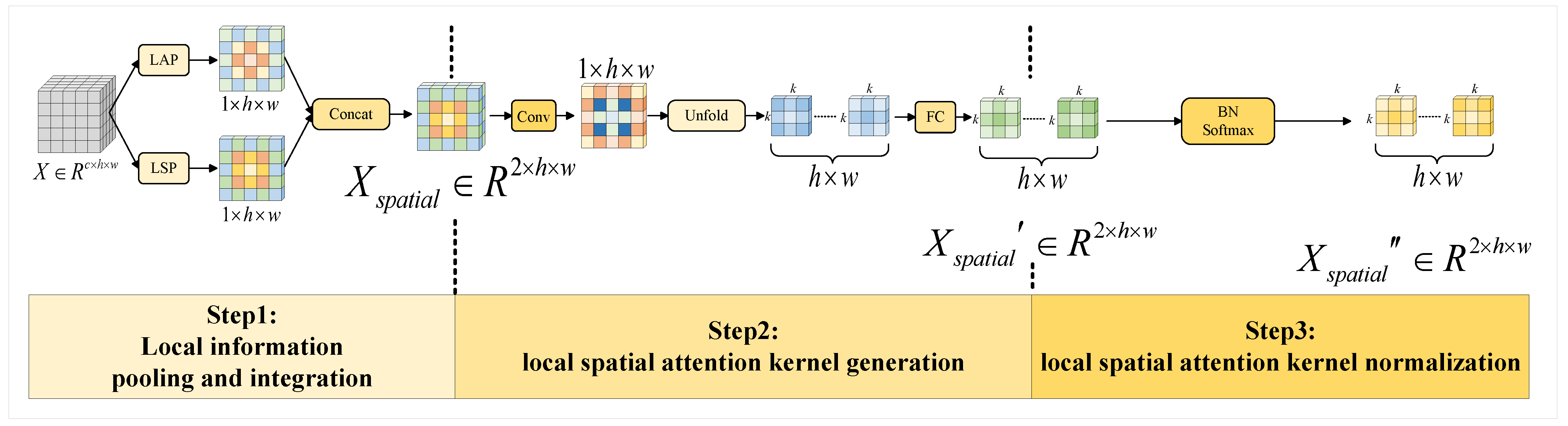
3.3. Local Spatial Attention Block

In the spatial branch, we focus on the relationship between each pixel in the space. We also utilize two statistics, the mean and standard deviation, to enhance information fusion across channels, similar to the global channel attention block. The method of obtaining the local spatial attention kernel is also a three-step process: local information pooling and integration, local spatial attention kernel generation, and local spatial attention kernel normalization. Local information pooling and integration for extracting an intermediate channel information representation is expressed as $X_{spatial}\in R^{d\times h\times w}$ from X, where d is the number of local features, and local spatial attention kernel generation is for generating a kernel ${X_{spatial}}^{\prime }\in R^{h\times w\times k\times k}$ from $X_{spatial}$. This is pretty much the same as global channel attention kernel normalization, although the local spatial attention kernel is also composed of a BN layer and a softmax activation function, which converts the original spatial attention weights ${X_{spatial}}^{″}\in R^{h\times w\times k\times k}$ from ${X_{spatial}}^{\prime }\in R^{h\times w\times k\times k}$ into probability distributions for the weighted combination of $k\times k$ neighborhoods across all spatial locations. The detailed structure of the local spatial attention block is illustrated in Figure 3.

Firstly, we perform the local information pooling and integration operation on the feature map $X\in R^{c\times h\times w}$ that fuses channel information, and thus we find the mean and variance of input X in the channel dimension, which are called local average pooling (LAP) and local standard deviation pooling (LSP), respectively. Two locally related statistics are obtained, denoted as ${\mu }_{local}\in R^{1\times h\times w}$ and ${\sigma }_{local}\in R^{1\times h\times w}$. By concatenating these two statistics $\left(d=2\right)$, the intermediate channel information representation $X_{spatial}\in R^{d\times h\times w}$ is calculated as follows:

$$X_{spatial}=\left[{\mu }_{local},{\sigma }_{local}\right].$$

(6)

Secondly, considering the efficiency and conceptual clarity, we adopted a three-layer network design consisting of a convolutional layer, an unfold operation, and a fully connected layer. The first convolutional layer is employed to adjust the channel dimension. Subsequently, the unfold operation generates the convolution kernel by extracting all $k\times k$ neighborhoods for each pixel in $X_{spatial}$. Finally, the last fully connected layer captures the complexity of the neighborhood features. Formally, the output of the local spatial attention kernel generation is calculated as follows:

$${X_{spatial}}^{\prime }=W_4\left(Unfold\left(W_3\left(X_{spatial}\right)\right)\right),$$

(7)

where

$$W_3\in R^{(2\times h\times w)\times (1\times h\times w)},$$

$$Unfold\in R^{(1\times h\times w)\times (h\times w\times k\times k)},$$

$$W_4\in R^{(h\times w\times k\times k)\times (h\times w\times k\times k)}.$$

Thirdly, similar to the normalization of global channel attention kernels, the normalization of local spatial attention kernels assesses the significance of global information within individual $k\times k$ neighborhoods across all spatial locations, thereby emphasizing or suppressing them accordingly. Formally, the local spatial attention kernel ${X_{spatial}}^{\prime }\in R^{h\times w\times k\times k}$ is calculated as follows:

$${X_{spatial}}^{″}=Softmax\left(BN\left(X_{spatial}^{\prime }\right)\right).$$

(8)

3.4. Fusion Module

We then fused the obtained global channel attention kernel in the fusion module with the local spatial attention kernel. Usually, in a specific task, we do not know how to assign these two types of weights to be more beneficial to the results or how to adjust the combination of addition and multiplication to be more beneficial to the results. Therefore, we used a more general form to weight these two types of weights, where $\lambda$ and $\gamma$ are two learnable parameters and both are required to be positive. By introducing these two parameters, the allocation of global channel attention weights and local spatial attention weights would be more appropriate. For simplicity, we define $channel\left(x\right)={X_{channel}}^{″}$ and $spatial\left(x\right)={X_{spatial}}^{″}$. The computation of the proposed fusion module is as follows:

$$GLAU\left(X\right)=\lambda \left(channel\right(X)+spatial(X\left)\right)+\gamma \left(channel\right(X)\times spatial(X\left)\right).$$

(9)

The parameter $\lambda$ controls the additive combination of the global channel attention kernel and local spatial attention kernel, while $\gamma$ does the same for their multiplicative combination.

Compared with existing methods, our dynamic convolutions have two important different characteristics. Firstly, our dynamic convolution kernels can be applied to integrate global and local information at each convolution layer. Secondly, our dynamic convolution kernels are adaptively learned from the input data according to the spatial and channel positions. Therefore, our dynamic convolution kernels are spatially specific and channel-specific. Thanks to the above two characteristics, our dynamic convolutions have a more efficient and accurate feature representation ability while requiring fewer learnable parameters. Modified CNNs incorporating GLAUs are referred to as “GLAUNets”.

3.5. Computational Complexity

In the following analysis, we use these notations: n is the number of pixels; c: is the channel number; k is the kernel size; and r is the squeeze ratio in the global channel attention block.

Table 1. Comparison of the parameter number, computational costs, and inference latency. “Params” means the number of parameters, “Time” represents the time complexity, and “Space” denotes the space complexity of the generated filters. “Latency” refers to the average inference time of the model, where the input to the feature map is $2\times 256\times 200\times 300$.

Kernel	Conv	DwConv	DDF	GLAU
Params	$c^2{k}^2$	$c{k}^2$	$c{k}^2+\sigma c^2\left(1+k^2\right)$	$2c{k}^2+\frac{6}{r}·c^2\left(6+k^2\right)$
Time	$O\left(n{c}^2{k}^2\right)$	$O\left(nc{k}^2\right)$	$O\left(nc{k}^2+c^2{k}^2\right)$	$O\left(nc{k}^2+c^2{k}^2\right)$
Space	–	–	$O\left(\left(n+c\right)k^2\right)$	$O\left(\left(n+c\right)k^2\right)$
Latency	12.7 ms	1.8 ms	5.2 ms	7.8 ms

shows a comparison of the parameter, space, time complexity, and average inference time between the standard convolution (Conv), depth-wise convolution (DwConv), the Decoupled Dynamic Filter (DDF) networks [42], and our GLAU method.

Number of parameters. In the DDF, it has $c{k}^2$ as the parameter for the spatial filter branch and $\sigma c^2\left(1+k^2\right)$ for the channel filter branch for a total of $c{k}^2+\sigma c^2\left(1+k^2\right)$ parameters. Similar to the DDF, our GLAU also has two branches. Among them, in the local spatial attention block, while first passing through a convolutional layer, this step has $2c$ parameters, and then throughout the unfold operation, this step has $k^2$ parameters. In the global channel attention block, for the first fully connected layer, we have $6c·\frac{6}{r}·c$ parameters, and the second fully connected layer has $\frac{6}{r}·c^2·k^2$ parameters. Overall, our GLAU has $2c{k}^2+\frac{6}{r}·c^2\left(6+k^2\right)$ parameters. Depending on the values of r, k, and c (usually set to 0.0625, 3, and 256, respectively), the number of parameters for the GLAU can be even lower than a standard convolution layer.

Time complexity. The GLAU’s local spatial attention block requires $4nc{k}^2$ floating-point operations (FLOPs), the global channel attention block requires $2·\frac{6}{r}·c^2\left(6+k^2\right)$ FLOPs, and the fusion module requires 2 FLOPs. In total, the GLAU requires $4nc{k}^2+2·\frac{6}{r}·c^2\left(6+k^2\right)+2$ FLOPs and $O\left(nc{k}^2+c^2{k}^2\right)$ for its time complexity. Because $n\gg c,k$, the term $c^2{k}^2$ can be ignored. Therefore, the time complexity of the GLAU is approximately equal to $O\left(nc{k}^2\right)$, which is similar to that of depth-wise convolution and better than a standard convolution with a time complexity of $O\left(n{c}^2{k}^2\right)$.

Space complexity. Standard and depth-wise convolutions do not generate content-adaptive kernels. The GLAU has design motivations similar to the DDF, as both have two branches. Therefore, the spatial complexities of the two are to the same order of magnitude.

Following the DDF [42], we re-compared the inference latency of the four methods on our devices (see Table 1). We had a slightly higher latency than DwConv and the DDF but a faster one than standard static convolution.

In conclusion, the GLAU has a time complexity similar to the DDF and significantly better than standard static convolution. It is worth noting that although GLAU generation involves a data-dependent convolutional kernel, the parameters of the GLAU are still much smaller than those of standard convolutional layers.

4. Experiments

This section evaluates the proposed GLAUNets with baseline methods and state-of-the-art dynamic convolution networks. In terms of different evaluation indicators, a series of experiments was carried out to demonstrate the effectiveness and merit of the proposed GLAUNets with different network architectures on different publicly available datasets.

4.1. Implementation Details

4.1.1. CIFAR, Mini-ImageNet, Caltech101, and DTD Datasets

The following experiments were performed on five datasets: CIFAR-10, CIFAR-100, Mini-ImageNet, Caltech101, and the Describable Textures Dataset (DTD).

Table 2. Summary of classification datasets.

Dateset	Image Size	Trainging Set	Validation Set	Class	BatchSize
CIFAR-10	32 × 32	50,000	10,000	10	32
CIFAR-100	32 × 32	50,000	10,000	100	32
Mini-ImageNet	64 × 64	50,000	10,000	100	32
Caltech101	112 × 112	6942	1736	101	64
DTD	112 × 112	4512	1128	47	64

shows that the CIFAR-10 dataset consists of 60,000 color images in 10 categories, with 6000 images in each category. The CIFAR-100 dataset is quite similar to CIFAR-10, except it has 100 classes, each containing 600 images. Mini-ImageNet dataset is more challenging than the CIFAR datasets. It is a subset of ImageNet with 100 classes containing 60,000 color images. The Caltech101 dataset contains images from 101 object classes, and for each object class, there are about 40–800 images, while most classes have about 50 images. The resolution of the images is about 300 × 200 pixels. The DTD contains 5640 texture images in 47 classes. The size of the images in the CIFAR dataset is 32 × 32, the images in the Mini-ImageNet dataset were resized and center-cropped to 64 × 64, and the Caltech101 dataset and DTD were similarly resized and center-cropped to 112 × 112 to match our computing resources.

4.1.2. Location of GLAU

All experiments were based on three main network architectures: ResNet [17], GoogLeNet [19], and ShuffluNetV2 [53]. There was a performance drop when we applied the GLAU to all layers of these architectures. This was expected, as the characteristics of the GLAU reduce the number of parameters and the model complexity of the network. Thus, we applied the GLAU to partial convolution layers to guarantee the network’s performance while significantly reducing the parameters. Specifically, we applied GLAUs to the second 3 × 3 convolutions at all basic block positions of the ResNet architectures. On GoogLeNet, we implemented GLAUs for all 3 × 3 convolutions. We also substituted the first depthwise convolutions of ShuffluNetV2 with GLAUs.

4.1.3. Parameter Fine-Tuning

For accurate comparisons, we used publicly available codes of existing model architectures. The GLAU was introduced to replace different convolutions in existing model architectures for image classification. All experiments were implemented under the Pytorch framework and were accelerated by an NVIDIA Quadro RTX 8000 GPU with 48 GB of video memory. All models were trained for 100 epochs using an SGD optimizer. The initial learning rate was set to 0.1 and divided by 10 at 60% and 90% of the total number of training epochs. Following [20], we used a weight decay of 1 × 10⁻⁴ and momentum of 0.9. For details about how to set the batch size, see Table 1. In addition, for the classification accuracy (Top 1 Acc and Top 5 ACC) in each experiment, we repeated them 10 times and took the average. We emphasize that we chose the same training configuration for all models to facilitate a fair comparison.

4.2. Comparison of Lightweight CNN and Multi-Branch CNN on Different Datasets

To compare GLAUNets with existing lightweight and multi-branch CNNs on ShuffleNetV2 and GoogLeNet, a series of experiments was conducted on the public image classification datasets CIFAR-10, CIFAR-100, Mini-ImageNet, Caltech101, and DTD. We analyzed the results through three evaluation indicators: classification accuracy (Top 1 Acc and Top 5 ACC), the number of parameters (Params), and computational complexity (FLOPs).

Table 3. Comparison of lightweight CNNs and multi-branch CNNs on different datasets. The results of our GLAU method are in bold. The numbers in parentheses refer to the increase compared with the baseline.

Model	Dataset	Baseline
		Params (M)	FLOPs (M)	Top 1 ACC (%)	Top 5 ACC (%)
ShuffleNetV2	CIFAR-10	1.26	11.82	87.89	99.61
	CIFAR-100	1.36	11.91	63.60	87.87
	Mini-ImageNet	1.36	47.35	60.90	84.76
	Caltech101	1.36	189.08	81.29	94.80
	DTD	1.30	189.02	56.11	84.40
GoogLeNet	CIFAR-10	5.99	1535.09	92.67	99.86
	CIFAR-100	6.08	1535.91	72.60	92.04
	Mini-ImageNet	6.08	6140.43	66.37	87.47
	Caltech101	6.08	24,561.42	74.87	90.56
	DTD	6.03	24,561.37	53.64	83.51
Model	Dataset	GLAUNets
		Params (M)	FLOPs (M)	Top 1 ACC (%)	Top 5 ACC (%)
ShuffleNetV2	CIFAR-10	1.79	12.76	88.08 (+0.19)	99.69 (+0.08)
	CIFAR-100	1.88	12.85	64.04 (+0.44)	88.14 (+0.27)
	Mini-ImageNet	1.88	49.64	61.68 (+0.78)	85.40 (+0.64)
	Caltech101	1.88	196.81	83.30 (+2.01)	95.87 (+1.07)
	DTD	1.88	196.81	57.18 (+1.07)	85.82 (+1.42)
GoogLeNet	CIFAR-10	3.92 (−34.5%)	853.03 (−44.4%)	93.59 (+0.92)	99.88 (+0.02)
	CIFAR-100	4.02 (−33.9%)	853.12 (−44.5%)	72.75 (+0.15)	93.18 (+1.14)
	Mini-ImageNet	4.02 (−33.9%)	3410.17 (−44.5%)	69.02 (+2.65)	89.49 (+2.02)
	Caltech101	4.02 (−33.9%)	13,638.36 (−44.5%)	77.35 (+2.48)	93.16 (+2.60)
	DTD	3.96 (−34.3%)	13,638.30 (−44.5%)	53.90 (+0.26)	84.04 (+0.53)

shows the evaluation results on CIFAR-10, CIFAR-100, Mini-ImageNet, Caltech101, and DTD. Across the entirety of Table 3, our GLAUNets achieved the highest classification accuracy compared with the baseline. First was ShuffleNetV2, a lightweight network that achieved higher classification accuracy at the cost of a few parameters and increased computational complexity. Second was GoogLeNet, a multi-branch network which could significantly improve classification accuracy while reducing the number of parameters and computational complexity. Specifically, GoogLeNet’s performance on the five datasets saw the Params and FLOPs reduced by about 34% and 44%, respectively, while the classification accuracy still improved by about 2%. It is worth mentioning that on Mini-ImageNet, our Top 1 ACC and Top 5 ACC increased by 2.65% and 2.02%, respectively. On the Caltech101 dataset, our Top 1 ACC and Top 5 ACC improved by 2.48% and 2.60%, respectively.

4.3. Comparison of Attention-Based CNN Models on Different Datasets

The following experiments evaluated using the GLAU as a building block in five well-known attention-based CNN models, including SE-ResNet [34], CBAM-ResNet [35], ECA-ResNet [38], CA-ResNet [36], and SRM-ResNet [54]. Two deep residual network (ResNet) architectures of different sizes were used in the experiments for each CIFAR dataset to make the results more generalizable.

Table 4. Comparative experiment of attention-based CNN model on CIFAR-10 dataset. The results of our GLAU method are in bold. The numbers in parentheses refer to the increase compared with the baseline.

Model	Baseline			GLAUNets
	Params (M)	FLOPs (M)	Top-1 ACC (%)	Params (M)	FLOPs (M)	Top-1 ACC (%)
ResNet18	27.24	0.18	91.19	14.90 (−45.3%)	0.13 (−27.8%)	91.38 (+0.19)
SE-ResNet18 [34]	27.29	0.18	91.27	14.96 (−45.2%)	0.13 (−27.8%)	91.53 (+0.26)
CBAM-ResNet18 [35]	27.56	0.18	91.93	15.23 (−44.7%)	0.13 (−27.8%)	91.98 (+0.05)
ECA-ResNet18 [38]	27.29	0.18	91.20	14.96 (−45.2%)	0.13 (−27.8%)	91.40 (+0.20)
CA-ResNet18 [36]	27.27	0.18	91.94	14.93 (−45.3%)	0.13 (−27.8%)	92.13 (+0.19)
SRM-ResNet18 [54]	27.24	0.18	92.08	14.90 (−45.3%)	0.13 (−27.8%)	92.91 (+0.83)
ResNet32	70.39	0.47	92.58	39.55 (−43.8%)	0.35 (−25.5%)	93.43 (+0.85)
SE-ResNet32 [34]	70.54	0.47	92.67	39.70 (−43.7%)	0.35 (−25.5%)	92.77 (+1.10)
CBAM-ResNet32 [35]	71.21	0.48	93.38	40.37 (−43.3%)	0.36 (−25.0%)	93.55 (+0.17)
ECA-ResNet32 [38]	70.54	0.47	92.68	39.70 (−43.7%)	0.35 (−25.5%)	92.76 (+0.08)
CA-ResNet32 [36]	70.47	0.47	92.24	39.63 (−43.8%)	0.35 (−25.5%)	92.45 (+0.21)
SRM-ResNet32 [54]	70.39	0.47	93.43	39.56 (−43.8%)	0.35 (−25.5%)	93.88 (+0.45)

,

Table 5. Comparative experiment of attention-based CNN model on CIFAR-100 dataset. The results of our GLAU method are in bold. The numbers in parentheses refer to the increase compared with the baseline.

Model	Baseline
	Params (M)	FLOPs (M)	Top 1 ACC (%)	Top 5 ACC (%)
ResNet18	27.24	0.18	66.39	90.53
SE-ResNet18 [34]	27.30	0.18	67.58	90.95
CBAM-ResNet18 [35]	27.57	0.18	66.45	90.32
ECA-ResNet18 [38]	27.30	0.18	65.86	90.63
CA-ResNet18 [36]	27.27	0.18	67.16	90.33
SRM-ResNet18 [54]	27.24	0.18	66.53	90.12
ResNet34	60.66	0.52	69.54	91.64
SE-ResNet34 [34]	60.77	0.52	70.44	91.94
CBAM-ResNet34 [35]	61.22	0.53	69.60	91.55
ECA-ResNet34 [38]	60.77	0.52	70.05	91.69
CA-ResNet34 [36]	60.74	0.52	70.14	91.44
SRM-ResNet34 [54]	60.67	0.52	69.73	91.36
Model	GLAUNets
	Params (M)	FLOPs (M)	Top 1 ACC (%)	Top 5 ACC (%)
ResNet18	14.91 (−45.3%)	0.13 (−27.8%)	66.72 (+0.33)	90.62 (+0.09)
SE-ResNet18 [34]	14.96 (−45.2%)	0.13 (−27.8%)	68.06 (+0.48)	91.15 (+0.20)
CBAM-ResNet18 [35]	15.23 (−44.8%)	0.14 (−22.2%)	66.83 (+0.38)	90.51 (+0.19)
ECA-ResNet18 [38]	14.96 (−45.2%)	0.13 (−27.8%)	65.98 (+0.12)	90.77 (+0.14)
CA-ResNet18 [36]	14.94 (−45.1%)	0.14 (−22.2%)	67.68 (+0.52)	90.64 (+0.31)
SRM-ResNet18 [54]	14.91 (−45.3%)	0.13 (−27.8%)	66.94 (+0.41)	90.46 (+0.34)
ResNet34	33.87 (−44.2%)	0.39 (−25.0%)	70.73 (+1.19)	92.29 (+0.65)
SE-ResNet34 [34]	33.98 (−44.1%)	0.39 (−25.0%)	70.56 (+0.12)	91.99 (+0.05)
CBAM-ResNet34 [35]	34.43 (−43.8%)	0.40 (−24.5%)	69.84 (+0.24)	91.76 (+0.21)
ECA-ResNet34 [38]	33.97 (−44.1%)	0.39 (−25.0%)	70.11 (+0.06)	91.74 (+0.05)
CA-ResNet34 [36]	33.94 (−44.1%)	0.39 (−25.0%)	70.32 (+0.18)	91.49 (+0.05)
SRM-ResNet34 [54]	33.87 (−44.2%)	0.39 (−25.0%)	70.23 (+0.50)	91.45 (+0.09)

and

Table 6. Comparative experiment of attention-based CNN model on Mini-ImageNet dataset. The results of our GLAU method are in bold. The numbers in parentheses refer to the increase compared with the baseline.

Model	Baseline
	Params (M)	FLOPs (M)	Top 1 ACC (%)	Top 5 ACC (%)
ResNet18	108.94	0.18	55.78	81.87
SE-ResNet18 [34]	109.17	0.18	56.46	81.78
CBAM-ResNet18 [35]	110.23	0.18	54.31	81.27
ECA-ResNet18 [38]	109.17	0.18	56.17	82.36
CA-ResNet18 [36]	109.00	0.18	56.11	82.09
SRM-ResNet18 [54]	108.95	0.18	56.68	82.36
Model	GLAUNets
	Params (M)	FLOPs (M)	Top 1 ACC (%)	Top 5 ACC (%)
ResNet18	59.45 (−45.4%)	0.13 (−27.8%)	55.88 (+0.10)	81.93 (+0.06)
SE-ResNet18 [34]	59.68 (−45.3%)	0.13 (−27.8%)	56.46 (+0.00)	81.86 (+0.08)
CBAM-ResNet18 [35]	60.74 (−44.9%)	0.14 (−22.2%)	54.50 (+0.19)	81.35 (+0.08)
ECA-ResNet18 [38]	59.68 (−45.3%)	0.13 (−27.8%)	56.21 (+0.04)	82.51 (+0.15)
CA-ResNet18 [36]	59.51 (−45.4%)	0.14 (−22.2%)	56.37 (+0.26)	82.05 (−0.04)
SRM-ResNet18 [54]	59.45 (−45.4%)	0.13 (−27.8%)	56.72 (+0.04)	82.29 (−0.07)

show the results of the attention-based ResNet architecture on CIFAR-10, CIFAR-100, and Mini-ImageNet, respectively. In almost every group of experiments, the GLAUNets had slightly improved classification accuracy while reducing the number of model parameters and computational complexity. For example, compared with the baseline, the number of parameters in GLAUNets and FLOPs was reduced by about 44% and 26% on the three datasets, respectively, but the classification accuracy could still be improved by about 1%.

4.4. Comparison of State-of-the-Art Dynamic Convolutions on Different Datasets

In this section, we apply the GLAU, standard convolution, and existing dynamic convolutions (DYconv [10], CondConv [9], Involution [44], DCD [51], OdConv [52], and the DDF [42]) to ResNet56 and compare their classification accuracy, number of parameters, and computational complexity.

Table 7. Comparative experiments with state-of-the-art dynamic convolution on the four different datasets.

Dataset	Model	Params (M)	FLOPs (M)	Top 1 ACC (%)	Top 5 ACC (%)
CIFAR-10	ResNet56	0.86	127.93	92.72	99.99
	DCD [51]	1.00	134.33	93.67	99.99
	DDF [42]	0.53	66.90	91.09	99.99
	OdConv [52]	0.48	64.54	91.23	99.99
	CondConv [9]	0.42	64.49	93.34	99.99
	DyConv [10]	0.43	64.50	93.83	99.99
	Involution [44]	0.44	66.84	90.46	99.99
	GLAUNets (ours)	0.64	72.42	93.30	99.99
Dataset	Model	Params (M)	FLOPs (M)	Top 1 ACC (%)	Top 5 ACC (%)
CIFAR-100	ResNet56	0.86	127.94	72.56	92.83
	DCD [51]	1.00	134.34	73.50	93.24
	DDF [42]	0.54	66.91	68.23	91.59
	OdConv [52]	0.48	64.55	65.81	89.66
	CondConv [9]	0.43	64.50	72.86	93.05
	DyConv [10]	0.44	64.51	72.32	92.69
	Involution [44]	0.44	66.84	64.46	89.37
	GLAUNets (ours)	0.65	72.43	72.19	93.08
Dataset	Model	Params (M)	FLOPs (M)	Top 1 ACC (%)	Top 5 ACC (%)
Caltech101	ResNet56	0.86	2046.89	75.22	91.03
	DCD [51]	1.00	2147.57	77.69	92.97
	DDF [42]	0.54	1069.06	72.50	89.26
	OdConv [52]	0.49	1031.87	64.43	84.43
	CondConv [9]	0.43	1031.81	74.86	90.50
	DyConv [10]	0.44	1031.82	77.64	90.27
	Involution [44]	0.44	1069.41	68.67	86.61
	GLAUNets (ours)	0.65	1155.28	75.98	91.56
Dataset	Model	Params (M)	FLOPs (M)	Top 1 ACC (%)	Top 5 ACC (%)
DTD	ResNet56	0.86	2046.89	50.80	82.98
	DCD [51]	1.00	2147.57	52.30	81.47
	DDF [42]	0.54	1069.06	51.86	81.29
	OdConv [52]	0.48	1031.86	50.08	79.88
	CondConv [9]	0.43	1031.81	50.18	79.34
	DyConv [10]	0.44	1031.82	50.71	80.85
	Involution [44]	0.44	1069.41	50.94	82.13
	GLAUNets (ours)	0.65	1155.28	52.04	83.78

shows the experimental results for different datasets.

4.4.1. Comparative Experiments with State-of-the-Art Dynamic Convolution on a Different Dataset

First, experiments were performed on the CIFAR-10 dataset using ResNet56, and the experimental results are presented in Table 7. Among them, the DCD method achieved the best classification accuracy, but it came at the cost of consuming more parameters and computational complexity. In our GLAU method, the trade-off between the three was that the classification accuracy was still improved by 0.58% to 93.3% with a reduction in the number of parameters by about 23% and the number of flops by about 43%, which is comparable to the state-of-the-art methods CondConv and DyConv.

Next, experiments were performed on the CIFAR-100 dataset using ResNet56, and the results are presented in Table 7. Among them, although the DCD method achieved the best classification accuracy, it consumed more parameters and computational complexity. However, our GLAU method achieved a classification accuracy of 93.3% in the Top 5 ACC with the addition of an acceptable number of parameters and computational complexity, which was comparable to that of the state-of-the-art method CondConv.

In addition, the GLAU had similar performance on the Caltech101 and DTD datasets. For example, in Caltech101, the highest Top 1 ACC was for DCD and DyConv, but DCD consumed more computing resources, and the Top 5 ACC of DyConv was lower, being even lower than that for the baseline. In the DTD dataset, the GLAU obtained the highest Top 1 ACC and Top 5 ACC at the expense of improving the tiny parameters and flops. Overall, the GLAU made a direct trade-off between model performance and complexity.

4.4.2. Visualization of Various State-of-the-Art Dynamic Convolution Methods

To better observe the influence of GLAUs on image classification, we applied the Grad-CAM [55] method to visualize different dynamic convolution networks and generate the corresponding heat maps. The input feature map was resized to 32 × 32. The results are shown in Figure 4. It is evident that compared with the other dynamic convolution methods, our method could focus on the target area and obtain more comprehensive information about it, resulting in effective performance.

4.5. Ablation Studies

We conducted a series of ablative experiments to comprehensively analyze the impact of different components on the proposed dynamic convolution with global and local attention.

4.5.1. Fusion Methods in GLAU: Optimizing Network Performance

In our GLAU method, the convolution kernel generated from two branches must go through a fusion module. To further verify the impact of different fusion methods on network performance, we considered the following four fusion methods: element-wise multiplication, element-wise addition, convex combination, and compounding of addition and multiplication. Specifically, we used ResNet44 for experiments on CIFAR-10 and ResNet20 for experiments on CIFAR-100. The experimental results in

Table 8. Comparison of the four fusion methods on different architectures and datasets.

Dataset/Model	Fusion Method	FLOPs (M)	Params (M)	Top 1 ACC (%)	Top 5 ACC (%)
CIFAR-10/ResNet44	Element-wise multiplication	55.99	0.50	92.71	99.99
	Element-wise addition	55.99	0.50	92.82	99.99
	Convex combination	55.99	0.50	92.90	99.99
	Compounding (ours)	55.99	0.50	93.06	99.99
CIFAR-100/ResNet20	Element-wise multiplication	23.12	0.21	67.46	91.19
	Element-wise addition	23.12	0.21	67.76	91.15
	Convex combination	23.12	0.21	68.17	91.32
	Compounding (ours)	23.12	0.21	68.41	91.62

show that the number of parameters and FLOPs were unaffected by different fusion methods and remained unchanged. However, in the case of addition and multiplication compounding, the classification accuracy was the highest. Ultimately, we used the compounding of addition and multiplication approach to fusion.

4.5.2. Optimizing ResNet Architectures with GLAUs: Convolutional Layer Replacement Strategies

It is also worth considering where to replace the original network architecture with a GLAU. Similarly, we experimented on CIFAR-10 using ResNet44 and on CIFAR-100 using ResNet20. Specifically, we replaced the first convolutional layer, the second convolutional layer, and two convolutional layers in the primary block of the ResNet network with GLAUs. As can be seen in the results in

Table 9. Effects of applying GLAUs to different layer locations.

Dataset	Model	1st 3 × 3 conv	2nd 3 × 3 conv	FLOPs (M)	Params (M)	Top 1 ACC (%)	Top 5 ACC (%)
CIFAR-10	ResNet44	Baseline		99.16	0.66	93.20	99.99
		✓		58.14	0.50	92.77	99.99
			✓	55.99	0.55	93.06	99.99
		✓	✓	14.97	0.34	88.25	99.99
CIFAR-100	ResNet20	Baseline		41.63	0.28	68.33	91.70
		✓		25.27	0.21	67.34	90.86
			✓	23.12	0.21	68.41	91.62
		✓	✓	6.77	0.14	60.68	87.68

, the Params and FLOPs decreased after replacing both convolutional layers simultaneously compared with the baseline. However, the classification accuracy decreased even more. In addition, replacing the first convolutional layer was not much different from replacing the second convolutional layer in terms of Params and FLOPs, but the latter would obtain higher accuracy. Ultimately, we chose to replace the second convolutional layer with a GLAU.

4.5.3. Optimizing GLAU Channel Branch: Impact of Compression Ratio on Model Performance

In the channel branch of the GLAU method, the compression ratio r controls the degree of information fusion between channels. The magnitude of the compression ratio directly affects the number of model parameters and, ultimately, the model’s performance. We used ResNet18, ResNet32, ResNet34, and ResNet56 to perform comparative experiments on three datasets and draw more detailed and comprehensive conclusions. From

Table 10. Impact of compression ratio on model performance.

Dataset	Model	FLOPs (M)	Params (M)	Top 1 ACC (%)	Top 5 ACC (%)
CIFAR-10	ResNet18	27.24	0.18	91.19	99.99
	GLAUNets (r = 2)	15.15	0.38	91.46	99.99
	GLAUNets (r = 4)	15.01	0.24	91.28	99.99
	GLAUNets (r = 8)	14.94	0.16	91.14	99.99
	GLAUNets (r = 16)	14.90	0.13	91.38	99.99
	GLAUNets (r = 32)	14.88	0.11	90.91	99.99
CIFAR-10	ResNet32	70.39	0.47	92.58	99.99
	GLAUNets (r = 2)	40.19	0.98	93.46	99.99
	GLAUNets (r = 4)	39.83	0.62	93.36	99.99
	GLAUNets (r = 8)	39.64	0.44	93.32	99.99
	GLAUNets (r = 16)	39.55	0.35	93.43	99.99
	GLAUNets (r = 32)	39.51	0.30	92.94	99.99
CIFAR-100	ResNet18	27.24	0.18	66.39	90.53
	GLAUNets (r = 2)	15.16	0.39	66.86	90.84
	GLAUNets (r = 4)	15.01	0.24	66.73	90.61
	GLAUNets (r = 8)	14.94	0.17	66.68	90.63
	GLAUNets (r = 16)	14.91	0.13	66.72	90.62
	GLAUNets (r = 32)	14.89	0.12	66.18	90.64
CIFAR-100	ResNet34	60.66	0.52	69.54	91.64
	GLAUNets (r = 2)	34.56	1.08	70.83	92.47
	GLAUNets (r = 4)	34.16	0.69	70.87	92.15
	GLAUNets (r = 8)	33.97	0.49	70.60	92.71
	GLAUNets (r = 16)	33.87	0.39	70.73	92.29
	GLAUNets (r = 32)	33.82	0.34	70.63	92.21
Mini-ImageNet	ResNet18	108.94	0.18	55.78	81.87
	GLAUNets (r = 2)	59.70	0.39	55.81	82.20
	GLAUNets (r = 4)	59.56	0.24	54.80	82.25
	GLAUNets (r = 8)	59.48	0.17	55.18	81.68
	GLAUNets (r = 16)	59.45	0.13	55.88	81.93
	GLAUNets (r = 32)	59.43	0.12	53.60	80.32
Mini-ImageNet	ResNet56	511.73	0.86	63.53	85.90
	GLAUNets (r = 2)	290.14	1.79	63.69	86.97
	GLAUNets (r = 4)	289.49	1.14	63.82	86.34
	GLAUNets (r = 8)	289.16	0.81	63.16	86.70
	GLAUNets (r = 16)	289.00	0.65	63.78	86.79
	GLAUNets (r = 32)	288.92	0.57	63.04	86.39

, it can be concluded that a small compression ratio led to an increase in accuracy, but it also brought about a problem: an increase in Params and FLOPs. To make a trade-off, we chose a compression ratio of 16, which ensured the model’s performance and dramatically reduced the Params and FLOPs.

5. Conclusions

This work introduced a novel dynamic convolution method called the Global and Local Attention Unit (GLAU). The GLAU can integrate global and local features and adaptively generate convolution kernels. The proposed dynamic convolution kernels are spatially specific and channel-specific, making full use of the statistical information of the feature map so that better data representation can be realized. Our experiments show that GLAUs can improve classification accuracy and reduce complexity.

The GLAU provides a dynamic convolution method that takes spatial and channel positions into account using the attention mechanism. The GLAU uses a plug-and-play approach which is invoked at any time to replace convolutional layers in other network architectures. For example, a GLAU can be used for object detection and instance segmentation. Mask R-CNN can be used as the detection framework, ResNet50 can be the backbone, and part of the convolutional layer in ResNet50 can be replaced with a GLAU. The GLAU is expected to play a role in many areas of machine vision. In the future, we will focus on applying and researching GLAUs in other computer vision tasks.

References

1. Krizhevsky, A.; Sutskever, I.; Hinton, G.E. Imagenet classification with deep convolutional neural networks. Adv. Neural Inf. Process. Syst. 2012, 25. [Google Scholar] [CrossRef]
2. Hu, H.; Gu, J.; Zhang, Z.; Dai, J.; Wei, Y. Relation networks for object detection. In Proceedings of the IEEE Conference on Computer Vision and Pattern Recognition, Salt Lake City, UT, USA, 18–22 June 2018; pp. 3588–3597. [Google Scholar]
3. Zhang, H.; Dana, K.; Shi, J.; Zhang, Z.; Wang, X.; Tyagi, A.; Agrawal, A. Context encoding for semantic segmentation. In Proceedings of the IEEE Conference on COMPUTER Vision and Pattern Recognition, Salt Lake City, UT, USA, 18–22 June 2018; pp. 7151–7160. [Google Scholar]
4. Wang, X.; Girshick, R.; Gupta, A.; He, K. Non-local neural networks. In Proceedings of the IEEE Conference on Computer Vision and Pattern Recognition, Salt Lake City, UT, USA, 18–22 June 2018; pp. 7794–7803. [Google Scholar]
5. Yi, C.; Ren, L.; Zhan, D.C.; Ye, H.J. Leveraging Cross-Modal Neighbor Representation for Improved CLIP Classification. arXiv 2024, arXiv:2404.17753. [Google Scholar]
6. Wu, H.; Zhao, S.; Huang, X.; Wen, C.; Li, X.; Wang, C. Commonsense Prototype for Outdoor Unsupervised 3D Object Detection. arXiv 2024, arXiv:2404.16493. [Google Scholar]
7. Yan, H.; Wu, M.; Zhang, C. Multi-Scale Representations by Varying Window Attention for Semantic Segmentation. arXiv 2024, arXiv:2404.16573. [Google Scholar]
8. Jia, X.; De Brabandere, B.; Tuytelaars, T.; Gool, L.V. Dynamic filter networks. Adv. Neural Inf. Process. Syst. 2016, 29. [Google Scholar] [CrossRef]
9. Yang, B.; Bender, G.; Le, Q.V.; Ngiam, J. Condconv: Conditionally parameterized convolutions for efficient inference. Adv. Neural Inf. Process. Syst. 2019, 32. [Google Scholar] [CrossRef]
10. Chen, Y.; Dai, X.; Liu, M.; Chen, D.; Yuan, L.; Liu, Z. Dynamic convolution: Attention over convolution kernels. In Proceedings of the IEEE/CVF Conference on Computer Vision and Pattern Recognition, Seattle, WA, USA, 13–19 June 2020; pp. 11030–11039. [Google Scholar]
11. Zhang, Y.; Zhang, J.; Wang, Q.; Zhong, Z. Dynet: Dynamic convolution for accelerating convolutional neural networks. arXiv 2020, arXiv:2004.10694. [Google Scholar]
12. Chen, J.; Wang, X.; Guo, Z.; Zhang, X.; Sun, J. Dynamic region-aware convolution. In Proceedings of the IEEE/CVF Conference on Computer Vision and Pattern Recognition, Nashville, TN, USA, 19–25 June 2021; pp. 8064–8073. [Google Scholar]
13. Li, C.; Yao, A. KernelWarehouse: Towards Parameter-Efficient Dynamic Convolution. arXiv 2023, arXiv:2308.08361. [Google Scholar]
14. Hu, J.; Huang, L.; Ren, T.; Zhang, S.; Ji, R.; Cao, L. You only segment once: Towards real-time panoptic segmentation. In Proceedings of the IEEE/CVF Conference on Computer Vision and Pattern Recognition, Vancouver, BC, Canada, 17–24 June 2023; pp. 17819–17829. [Google Scholar]
15. Lin, M.; Chen, Q.; Yan, S. Network in network. arXiv 2013, arXiv:1312.4400. [Google Scholar]
16. Yu, F.; Koltun, V. Multi-scale context aggregation by dilated convolutions. arXiv 2015, arXiv:1511.07122. [Google Scholar]
17. He, K.; Zhang, X.; Ren, S.; Sun, J. Deep residual learning for image recognition. In Proceedings of the IEEE Conference on Computer Vision and Pattern Recognition, Las Vegas, NV, USA, 27–30 June 2016; pp. 770–778. [Google Scholar]
18. Simonyan, K.; Zisserman, A. Very deep convolutional networks for large-scale image recognition. arXiv 2014, arXiv:1409.1556. [Google Scholar]
19. Szegedy, C.; Liu, W.; Jia, Y.; Sermanet, P.; Reed, S.; Anguelov, D.; Erhan, D.; Vanhoucke, V.; Rabinovich, A. Going deeper with convolutions. In Proceedings of the IEEE Conference on Computer Vision and Pattern Recognition, Boston, MA, USA, 7–12 June 2015; pp. 1–9. [Google Scholar]
20. Huang, G.; Liu, Z.; Van Der Maaten, L.; Weinberger, K.Q. Densely connected convolutional networks. In Proceedings of the IEEE Conference on Computer Vision and Pattern Recognition, Honolulu, HI, USA, 21–26 July 2017; pp. 4700–4708. [Google Scholar]
21. Zagoruyko, S.; Komodakis, N. Wide residual networks. arXiv 2016, arXiv:1605.07146. [Google Scholar]
22. Li, J.; Fang, F.; Mei, K.; Zhang, G. Multi-scale residual network for image super-resolution. In Proceedings of the European Conference on Computer Vision (ECCV), Munich, Germany, 8–14 September 2018; pp. 517–532. [Google Scholar]
23. Xie, S.; Girshick, R.; Dollár, P.; Tu, Z.; He, K. Aggregated residual transformations for deep neural networks. In Proceedings of the IEEE Conference on Computer Vision and Pattern Recognition, Honolulu, HI, USA, 21–26 July 2017; pp. 1492–1500. [Google Scholar]
24. Liu, Z.; Mao, H.; Wu, C.Y.; Feichtenhofer, C.; Darrell, T.; Xie, S. A convnet for the 2020s. In Proceedings of the IEEE/CVF Conference on Computer Vision and Pattern Recognition, New Orleans, LA, USA, 18–24 June 2022; pp. 11976–11986. [Google Scholar]
25. Dosovitskiy, A.; Beyer, L.; Kolesnikov, A.; Weissenborn, D.; Zhai, X.; Unterthiner, T.; Dehghani, M.; Minderer, M.; Heigold, G.; Gelly, S.; et al. An image is worth 16 × 16 words: Transformers for image recognition at scale. arXiv 2020, arXiv:2010.11929. [Google Scholar]
26. Liu, Z.; Lin, Y.; Cao, Y.; Hu, H.; Wei, Y.; Zhang, Z.; Lin, S.; Guo, B. Swin transformer: Hierarchical vision transformer using shifted windows. In Proceedings of the IEEE/CVF International Conference on Computer Vision, Montreal, BC, Canada, 11–17 October 2021; pp. 10012–10022. [Google Scholar]
27. Peng, J.; Liu, Y.; Tang, S.; Hao, Y.; Chu, L.; Chen, G.; Wu, Z.; Chen, Z.; Yu, Z.; Du, Y.; et al. Pp-liteseg: A superior real-time semantic segmentation model. arXiv 2022, arXiv:2204.02681. [Google Scholar]
28. Wang, F.; Jiang, M.; Qian, C.; Yang, S.; Li, C.; Zhang, H.; Wang, X.; Tang, X. Residual attention network for image classification. In Proceedings of the IEEE Conference on Computer Vision and Pattern Recognition, Honolulu, HI, USA, 21–26 July 2017; pp. 3156–3164. [Google Scholar]
29. Han, J.; Gao, Y.; Lin, Z.; Yan, K.; Ding, S.; Gao, Y.; Xia, G.S. Dual Relation Mining Network for Zero-Shot Learning. arXiv 2024, arXiv:2405.03613. [Google Scholar]
30. Li, J.; Zhang, Z.; Zuo, W. TBSN: Transformer-Based Blind-Spot Network for Self-Supervised Image Denoising. arXiv 2024, arXiv:2404.07846. [Google Scholar]
31. Mansourian, A.M.; Jalali, A.; Ahmadi, R.; Kasaei, S. Attention-guided Feature Distillation for Semantic Segmentation. arXiv 2024, arXiv:2403.05451. [Google Scholar]
32. Pathak, D.; Krahenbuhl, P.; Donahue, J.; Darrell, T.; Efros, A.A. Context encoders: Feature learning by inpainting. In Proceedings of the IEEE Conference on Computer Vision and Pattern Recognition, Las Vegas, NV, USA, 27–30 June 2016; pp. 2536–2544. [Google Scholar]
33. Jaderberg, M.; Simonyan, K.; Zisserman, A. Spatial transformer networks. Adv. Neural Inf. Process. Syst. 2015, 28. [Google Scholar] [CrossRef]
34. Hu, J.; Shen, L.; Sun, G. Squeeze-and-excitation networks. In Proceedings of the IEEE Conference on Computer Vision and Pattern Recognition, Salt Lake City, UT, USA, 18–22 June 2018; pp. 7132–7141. [Google Scholar]
35. Woo, S.; Park, J.; Lee, J.Y.; Kweon, I.S. Cbam: Convolutional block attention module. In Proceedings of the European conference on computer vision (ECCV), Munich, Germany, 8–14 September 2018; pp. 3–19. [Google Scholar]
36. Hou, Q.; Zhou, D.; Feng, J. Coordinate attention for efficient mobile network design. In Proceedings of the IEEE/CVF Conference on Computer Vision and Pattern Recognition, Nashville, TN, USA, 19–25 June 2021; pp. 13713–13722. [Google Scholar]
37. Li, X.; Wang, W.; Hu, X.; Yang, J. Selective kernel networks. In Proceedings of the IEEE/CVF Conference on Computer Vision and Pattern Recognition, Long Beach, CA, USA, 15–20 June 2019; pp. 510–519. [Google Scholar]
38. Wang, Q.; Wu, B.; Zhu, P.; Li, P.; Zuo, W.; Hu, Q. ECA-Net: Efficient channel attention for deep convolutional neural networks. In Proceedings of the IEEE/CVF Conference on Computer Vision and Pattern Recognition, Seattle, WA, USA, 13–19 June 2020; pp. 11534–11542. [Google Scholar]
39. Ma, X.; Guo, J.; Tang, S.; Qiao, Z.; Chen, Q.; Yang, Q.; Fu, S. DCANet: Learning connected attentions for convolutional neural networks. arXiv 2020, arXiv:2007.05099. [Google Scholar]
40. Dai, J.; Qi, H.; Xiong, Y.; Li, Y.; Zhang, G.; Hu, H.; Wei, Y. Deformable convolutional networks. In Proceedings of the IEEE International Conference on Computer Vision, Venice, Italy, 22–29 October 2017; pp. 764–773. [Google Scholar]
41. Chen, J.; He, T.; Zhuo, W.; Ma, L.; Ha, S.; Chan, S.H.G. Tvconv: Efficient translation variant convolution for layout-aware visual processing. In Proceedings of the IEEE/CVF Conference on Computer Vision and Pattern Recognition, New Orleans, LA, USA, 18–24 June 2022; pp. 12548–12558. [Google Scholar]
42. Zhou, J.; Jampani, V.; Pi, Z.; Liu, Q.; Yang, M.H. Decoupled dynamic filter networks. In Proceedings of the IEEE/CVF Conference on Computer Vision and Pattern Recognition, Nashville, TN, USA, 19–25 June 2021; pp. 6647–6656. [Google Scholar]
43. Ha, D.; Dai, A.; Le, Q.V. Hypernetworks. arXiv 2016, arXiv:1609.09106. [Google Scholar]
44. Li, D.; Hu, J.; Wang, C.; Li, X.; She, Q.; Zhu, L.; Zhang, T.; Chen, Q. Involution: Inverting the inherence of convolution for visual recognition. In Proceedings of the IEEE/CVF Conference on Computer Vision and Pattern Recognition, Nashville, TN, USA, 19–25 June 2021; pp. 12321–12330. [Google Scholar]
45. Jiang, Z.H.; Yu, W.; Zhou, D.; Chen, Y.; Feng, J.; Yan, S. Convbert: Improving bert with span-based dynamic convolution. Adv. Neural Inf. Process. Syst. 2020, 33, 12837–12848. [Google Scholar]
46. Huang, Z.; Zhang, Z.; Lan, C.; Zha, Z.J.; Lu, Y.; Guo, B. Adaptive Frequency Filters As Efficient Global Token Mixers. In Proceedings of the IEEE/CVF International Conference on Computer Vision, Paris, France, 2–6 October 2023; pp. 6049–6059. [Google Scholar]
47. Ngo, T.D.; Hua, B.S.; Nguyen, K. ISBNet: A 3D point cloud instance segmentation network with instance-aware sampling and box-aware dynamic convolution. In Proceedings of the IEEE/CVF Conference on Computer Vision and Pattern Recognition, Vancouver, BC, Canada, 17–24 June 2023; pp. 13550–13559. [Google Scholar]
48. Xie, X.; Cui, Y.; Ieong, C.I.; Tan, T.; Zhang, X.; Zheng, X.; Yu, Z. Fusionmamba: Dynamic feature enhancement for multimodal image fusion with mamba. arXiv 2024, arXiv:2404.09498. [Google Scholar]
49. Song, Y.; Cao, Z.; Xiang, W.; Long, S.; Yang, B.; Ge, H.; Liang, Y.; Wu, C. Troublemaker Learning for Low-Light Image Enhancement. arXiv 2024, arXiv:2402.04584. [Google Scholar]
50. Yue, H.; Zhang, Z.; Mu, D.; Dang, Y.; Yin, J.; Tang, J. Full-frequency dynamic convolution: A physical frequency-dependent convolution for sound event detection. arXiv 2024, arXiv:2401.04976. [Google Scholar]
51. Li, Y.; Chen, Y.; Dai, X.; Liu, M.; Chen, D.; Yu, Y.; Yuan, L.; Liu, Z.; Chen, M.; Vasconcelos, N. Revisiting dynamic convolution via matrix decomposition. arXiv 2021, arXiv:2103.08756. [Google Scholar]
52. Li, C.; Zhou, A.; Yao, A. Omni-dimensional dynamic convolution. arXiv 2022, arXiv:2209.07947. [Google Scholar]
53. Ma, N.; Zhang, X.; Zheng, H.T.; Sun, J. Shufflenet v2: Practical guidelines for efficient cnn architecture design. In Proceedings of the European Conference on Computer Vision (ECCV), Munich, Germany, 8–14 September 2018; pp. 116–131. [Google Scholar]
54. Lee, H.; Kim, H.E.; Nam, H. Srm: A style-based recalibration module for convolutional neural networks. In Proceedings of the IEEE/CVF International Conference on Computer Vision, Seoul, Republic of Korea, 27 October–2 November 2019; pp. 1854–1862. [Google Scholar]
55. Selvaraju, R.R.; Cogswell, M.; Das, A.; Vedantam, R.; Parikh, D.; Batra, D. Grad-cam: Visual explanations from deep networks via gradient-based localization. In Proceedings of the IEEE International Conference on Computer Vision, Venice, Italy, 22–29 October 2017; pp. 618–626. [Google Scholar]
Figure 1. The structure of the GLAU.
Mathematics 12 01856 g001
Figure 2. Global channel attention block.
Mathematics 12 01856 g002
Figure 3. Local spatial attention block.
Mathematics 12 01856 g003
Figure 4. Grad-CAM visualization results. They are best viewed in color.
Mathematics 12 01856 g004