Review

An In-Depth Review of the Weibull Model with a Focus on Various Parameterizations

by
Yolanda M. Gómez
1,†,
Diego I. Gallardo
1,*,†,
Carolina Marchant
2,†,
Luis Sánchez
3,† and
Marcelo Bourguignon
4,†
1
Departamento de Estadística, Facultad de Ciencias, Universidad del Bío-Bío, Concepción 4081112, Chile
2
Faculty of Basic Sciences, Universidad Católica del Maule, Talca 3480112, Chile
3
Institute of Statistics, Universidad Austral de Chile, Valdivia 5110566, Chile
4
Statistics Department, Federal University of Rio Grande do Norte, Natal 59078-970, RN, Brazil
*
Author to whom correspondence should be addressed.
These authors contributed equally to this work.
Mathematics 2024, 12(1), 56; https://doi.org/10.3390/math12010056
Submission received: 8 November 2023 / Revised: 12 December 2023 / Accepted: 21 December 2023 / Published: 23 December 2023
(This article belongs to the Special Issue Probability, Statistics & Symmetry)

Abstract

:
The Weibull distribution is a versatile probability distribution widely applied in modeling the failure times of objects or systems. Its behavior is shaped by two essential parameters: the shape parameter and the scale parameter. By manipulating these parameters, the Weibull distribution adeptly captures diverse failure patterns observed in real-world scenarios. This flexibility and broad applicability make it an indispensable tool in reliability analysis and survival modeling. This manuscript explores five parameterizations of the Weibull distribution, each based on different moments, like mean, quantile, and mode. It meticulously characterizes each parameterization, introducing a novel one based on the model’s mode, along with its hazard and survival functions, shedding light on their unique properties. Additionally, it delves into the interpretation of regression coefficients when incorporating regression structures into these parameterizations. It is analytically established that all five parameterizations define the same log-likelihood function, underlining their equivalence. Through Monte Carlo simulation studies, the performances of these parameterizations are evaluated in terms of parameter estimations and residuals. The models are further applied to real-world data, illustrating their effectiveness in analyzing material fatigue life and survival data. In summary, this manuscript provides a comprehensive exploration of the Weibull distribution and its various parameterizations. It offers valuable insights into their applications and implications in modeling failure times, with potential contributions to diverse fields requiring reliability and survival analysis.

1. Background

The Weibull distribution is a popular continuous probability distribution that is commonly utilized to model the lifetimes or failure times of objects or systems. It was initially introduced by Waloddi Weibull in 1951 [1] and has since found applications in various fields. For instance, in reliability engineering, Keshevan et al. [2] employed the Weibull distribution to model the Hertzian fracture of Pyrex glass. In another study, Queeshi and Sheikh [3] used the Weibull distribution to analyze adhesive wear in metals. Similarly, Durham and Padgett [4] applied the distribution to carbon fibers and small composite specimens. Almeida [5] investigated the failure of coating using the Weibull distribution, while Fok et al. [6] focused on its use for brittle material. Additionally, Newell et al. [7] employed the distribution to study compressive failure in high-performance polymers and Li et al. [8] analyzed concrete components using the Weibull distribution.
The distribution mentioned above has been widely applied as a flexible modeling tool in various fields, addressing a diverse range of issues. It has been successfully utilized in disciplines such as quality control, weather forecasting, industrial engineering, electric systems engineering, communications systems engineering, hydrology, and more. For instance, Bebbington and Lai [9] utilized it for volcanic eruptions, while Durrans [10] and Heo et al. [11] applied it to regional flood frequency analysis. Fleming [12] used it to describe the dynamics of foliage biomass on Scots pine. In the field of Economics, Roed and Zhang [13] employed it to analyze unemployment duration data. In the context of wireless communications, the Weibull distribution is very flexible. Ikki and Ahmed [14] analyzed the performance of multi-hop relaying systems over Weibull fading channels in terms of bit error rate and outage probability. A similar analysis of the bit error rate and outage probability over multi-hop Weibull fading channels was also conducted by Wang et al. [15].
The Weibull distribution is defined by two parameters: the shape parameter ( ν ) and the scale parameter ( λ ). The shape parameter determines the shape of the distribution curve, while the scale parameter determines the characteristic magnitude or scale of the failure times. Depending on the value of the shape parameter ν , the Weibull distribution can exhibit different shapes. When ν > 1 , the distribution is positively skewed, indicating a decreasing failure rate over time. This shape is commonly known as the bathtub curve and is often observed in reliability analysis. In this curve, failures are more likely to occur either early on, due to manufacturing defects or initial wear, or in the later stages, due to aging or wear-out effects. When ν = 1 , the distribution simplifies to the exponential distribution, which is the only continuous distribution with a constant hazard function on the positive axis. For ν < 1 , the distribution is negatively skewed, indicating an increasing failure rate over time (Rinne [16]).
The versatility and importance of this distribution can be seen in its close relationship with several well-known distributions in statistics. It includes other distributions as special cases, such as the exponential distribution (when the shape parameter ν is equal to 1) and the Rayleigh distribution (when ν is equal to 2). Furthermore, if T follows a Weibull distribution, then Y = λ 1 ν log ( T / ν ) follows an extreme-value distribution. By applying a simple log transformation, the Weibull distribution can also be converted into the Gumbel distribution. Additionally, it acts as a limit distribution for the Burr distribution, establishing a significant connection between these distributions (Lai and Xie [17]). These relationships further emphasize the importance and wide-ranging applicability of the Weibull distribution in statistical modeling and analysis.
The Weibull distribution is widely used in modeling lifetimes because it can effectively represent different failure patterns observed in real-life situations. Failure data can be classified into two types: complete data and incomplete (censored) data. Complete data refer to cases where the actual observed values are known for every observation in the dataset. On the other hand, censored data occur when the actual observed values are unknown for some or all of the observations. It is worth noting that there are various types of censoring; more information can be found in the work by Lawless [18]. Several studies have examined the application of the Weibull distribution in analyzing censored data. For example, Ghitany et al. (2005) [19] and Klakattawi (2022) [20] extended the Weibull model and applied it to bladder cancer data, Joarder (2011) [21] and Jia et al. (2016) [22] studied leukemia data, and Lee et al. (2007) [23] focused on the head-and-neck-cancer trial. The Weibull distribution has an intriguing application in models involving a fraction of cure. This distribution is particularly well-suited for estimating the time it takes for cancer cells to produce detectable cancer. As a result, it has gained significant popularity in this field. Several studies, including those by Chen et al. [24], Yin and Ibrahim [25], Rodrigues et al. [26], Gallardo et al. [27], and Azimi et al. [28], have extensively explored this topic.
There are numerous extensions, generalizations, and modifications to the Weibull distribution. These developments have emerged to address the requirements of empirical datasets that exhibit characteristics beyond what can be effectively captured by a standard two-parameter Weibull model (Lai and Xie [17]). These extended models can be broadly classified into three groups: univariate, multivariate, and stochastic process models. Univariate models focus on enhancing the flexibility of the Weibull distribution for single variable analysis. Multivariate models extend the Weibull framework to handle multiple variables and their dependencies. Stochastic process models delve into time-dependent and dynamic variations of the Weibull distribution. Noteworthy references, such as Murthy et al. [29,30], provide insights into these diverse extensions and shed light on the advancements made in modeling techniques beyond the traditional Weibull framework. Silva et al. [31] derived the power-series extended Weibull class of distributions. Santos-Neto et al. [32] and Nascimento et al. [33] introduced a family of distributions encompassing well over forty variants. For more details about the generalizations and modifications of the Weibull distribution, see Murthy [30], Nadarajah and Kotz [34], Pham and Lai [35], and Almalki and Nadarajah [36], as well as the references therein. The analysis of the truncated Weibull distribution has been explored in many papers. For example, Wingo [37] proposed the left-truncated Weibull distribution. The right-truncated Weibull distribution has been analyzed by Zhang and Xie [38]. The doubly-truncated Weibull distribution has been studied in work by McEwen and Parresol [39].
In summary, the Weibull distribution is a versatile probability distribution that finds widespread application in modeling the failure times of objects or systems. The distribution’s characteristics and behaviors are determined by two key parameters: the shape parameter and the scale parameter. The shape parameter governs the shape of the distribution, allowing it to range from exponential to highly skewed distributions. On the other hand, the scale parameter influences the location and spread of the distribution. By manipulating these parameters, the Weibull distribution can effectively capture various failure patterns observed in real-world scenarios. Its flexibility and wide range of applications make it a valuable tool in reliability analysis and survival modeling.
The main objectives of this manuscript are as follows:
1.
We perform a review of the different parameterizations of the Weibull distribution documented in the literature, including the interpretation of the regression coefficients, when incorporating regression structures into these parameterizations.
2.
We introduce a novel parameterization of the Weibull model based on the mode of this distribution.
3.
We theoretically explore the equivalence of the five parameterizations of the Weibull distribution in the context of regression models, since there is no discussion connecting all the mentioned parameterizations.
The manuscript is organized as follows. In Section 2, five parameterizations of the Weibull distribution are introduced. Three of these parameterizations are mean-based, one is quantile-based, and the last one is mode-based. Each parameterization is characterized by examining the respective hazard and survival functions. Section 3 delves into the interpretation of regression coefficients when regression structures are incorporated into the parameters of the five Weibull model parameterizations. In Section 5, we analytically demonstrate that the five parameterizations of the Weibull model discussed in the previous section define the same log-likelihood function. Section 6 presents Monte Carlo (MC) simulation studies for parameter estimation and residuals. In Section 6, the analyzed models are applied to real data. Specifically, two illustrations are provided to exemplify their applicability and use in material fatigue life and survival data. should be noted that all models have been implemented using the R-project code (https://www.r-project.org/, accessed on 5 December 2023). Finally, Section 7 summarizes the main conclusions of the manuscript and discusses possible avenues for future work.

2. Weibull Parameterizations

As discussed in Section 1, the Weibull distribution is one of the most used models in reliability analysis because it is a parsimonious model with a simple expression for the density, survival, and hazard functions, and with some interesting properties. For instance, it can assume a decreasing, increasing, or constant hazard rate, depending only on the shape parameter ν (<1, >1, or =1, respectively). However, the Weibull distribution has many parameterizations in the literature, depending on the study.
The accelerated failure time (AFT) model, which is employed as the base parameterization, is used for the Weibull model; it has hazard and survival functions given by
h ( t ; λ , ν ) = ν λ t λ ν 1 , t , ν , λ > 0 .
and
S ( t ; λ , ν ) = exp t λ ν , t , ν , λ > 0 ,
respectively, with λ and ν parameters of scale and shape, respectively. This parameterization is referred to as WEI ( λ , ν ) . An alternative parameterization of the Weibull model is associated with the proportional hazards model, in which the hazard and survival functions are given by
h ( t ; λ , ν ) = ν λ t ν 1 , t , ν , λ > 0
and
S ( t ; λ , ν ) = exp λ t ν , t , ν , λ > 0 ,
respectively. This parameterization is referred to as WEI2 ( λ , ν ) , where λ and ν act as the scale and shape parameters, respectively. A third alternative parameterization of the Weibull model is related to its mean. Fernandes et al. [40] propose a reparameterization that expresses the Weibull distribution in terms of the process mean, enabling straightforward monitoring of the Weibull mean. In this parameterization, the hazard and survival functions are given by
h ( t ; λ , ν ) = ν γ t γ ν 1 , t , ν , λ > 0
where γ = λ / Γ ( 1 + 1 / ν ) and
S ( t ; λ , ν ) = exp t γ ν , t , ν , λ > 0 ,
respectively. This parameterization is referred to as WEI3 ( λ , ν ) . In this case, E ( T ) = λ .
Recently, a fourth parameterization for the Weibull distribution was introduced by Sánchez et al. [41]. In this parameterization, the hazard and survival functions are given by
h ( t ; λ , ν ) = log ( 1 q ) ν λ t λ ν 1 , t , ν , λ > 0 .
where q ( 0 , 1 ) and
S ( t ; λ , ν ) = exp log ( 1 q ) t λ ν , t , ν , λ > 0 ,
respectively. This parameterization is referred to as WEI4 ( λ , ν ) . In this case, λ represents the q-quantile of the distribution.
Alternatively, a fifth parameterization of the Weibull is proposed, based on its mode. The main motivation for re-parameterizing the model in terms of this measure is associated with the robustness of the mode (above the mean, for example) and the fact that it is a measure that has been used more frequently in the literature in recent years. For instance, see Yao and Li [42], Chen [43], and Bourguignon et al. [44]. In this parameterization, the hazard and survival functions are given by
h ( t ; λ , ν ) = [ ν 1 ] λ t λ ν 1 , t , ν , λ > 0 .
and
S ( t ; λ , ν ) = exp 1 1 ν t λ ν , t , λ > 0 , ν > 1 .
This parameterization is referred to as WEI5 ( λ , ν ) . In this case, λ represents the mode of the distribution. Table 1 presents the mean, mode, q-quantile, and variance for the five parameterizations of the Weibull distribution explored in this study.
For a set of p covariates observed for each individual and the intercept term, say x i = ( 1 , x 1 i , x 2 i , , x p i ) , and for the four parameterizations, it is typical to include a regression structure in λ , as follows
λ i = g x i β , i = 1 , , n ,
where β = ( β 0 , β 1 , β 2 , , β p ) , and g ( · ) is a twice differentiable function, such as g : R R + . The most common choice is g ( u ) = exp ( u ) , which also facilitates the interpretation of the regression coefficients. In each model, such interpretation depends on its specific parameterization (WEI, WEI2, WEI3, WEI4, and WEI5). However, it will be demonstrated that when a regression structure is incorporated solely into λ , as in Equation (1), without affecting the shape parameter ν , then all five models share the same probability density function (PDF) and, consequently, the same log-likelihood function. Furthermore, it will also be demonstrated that introducing a dual regression structure for both λ and ν in the WEI, WEI2, WEI3, and WEI4 models results in different PDFs among the models.

3. Interpretation of the Coefficients

In this section, we explore the varying interpretations of regression coefficients in the Weibull model across different parameterizations. Let us consider two individuals with associated covariates, x i = ( 1 , x i 1 , , x i j , , x i p ) and x i * = ( 1 , x i 1 , , x i j + 1 , , x i p ) , which is that x i and x i * are identical, except for an increase of one unit in the j-th covariate. The scenario where the j-th covariate is quantitative will be focused on. However, in all cases, a similar interpretation can be applied to x i j , assuming two categories (labeled as 0 and 1). Note that x i * β = x i β + β j .

3.1. WEI Model

For the AFT parameterization, we obtain
S ( t ; λ i , ν ) = exp t λ i ν = S 0 ( λ i 1 t ; ν ) , t > 0 ,
where S 0 ( t ) = exp ( t ν ) . In this context, λ i 1 is known as the accelerator factor. More precisely, as mentioned by Kleinbaum and Klein [45], “the accelerator factor is a ratio of survival times corresponding to any fixed value of S ( t ) ”. In this case, to facilitate the interpretation of the coefficients, it is set g ( u ) = exp ( u ) . Consequently, the interpretations of covariates are as follows: If exp ( β j ) = 2 , then the median survival time doubles when the j-th covariate is increased by one unit, compared to the median survival time when the j-th covariate remains unchanged.
Remark 1. 
For WEI2, WEI3, and WEI4 parameterizations, the traditional link function is g ( u ) = exp ( u ) .

3.2. WEI2 Model

In this case, the quotient between the hazard function related to x i and x i * is
h ( t ; x i , ν ) h ( t ; x i * , ν ) = exp ( x i * β ) ν t ν 1 exp ( x i β ) ν t ν 1 = exp ( β j ) .
This does not depend on t (hence, the name ‘proportional hazard models’). Therefore, exp ( β j ) should be interpreted as the increase (or decrease) in the hazard function when the j-th covariate increases by one unit.

3.3. WEI3 Model

In this case, the expected value of the distribution is E ( T i ; x i ) = λ i . Therefore, the quotient between the mean related to x i and x i * is
E ( T i ; x i * ) E ( T i ; x i ) = exp ( x i * β ) exp ( x i β ) = exp ( β j ) .
Therefore, exp ( β j ) should be interpreted as the percentage increase (or decrease) in the mean when the j-th covariate is increased by one unit.

3.4. WEI4 Model

In this case, the 100 × q -th quantile of the distribution is τ q ( x i ) = λ i . Therefore, the quotient between the 100 × q -th quantile related to x i and x i * is given by
τ q ( x i * ) τ q ( x i ) = exp ( x i * β ) exp ( x i β ) = exp ( β j ) .
Then, exp ( β j ) represents the percentage increase (or decrease) in the 100 × q -th quantile when the j-th covariate is increased by one unit.

3.5. WEI5 Model

For this model, the mode of the distribution is Mo ( T i ; x i ) = λ i . Therefore, the model related to x i and x i * is
Mo ( T i ; x i * ) Mo ( T i ; x i * ) = exp ( x i * β ) exp ( x i β ) = exp ( β j ) .
In this case, exp ( β j ) represents the percentage increase (or decrease) in the mode when the j-th covariate is increased by one unit.

3.6. The Bi-Univocity among the Four Parameterizations When Modeling Only λ

To date, there is no discussion in the literature about the connection between the different parameterizations of the Weibull distribution when incorporating regression structures into these parameterizations. The following theorem establishes the biunivocal relationship between the WEI, WEI2, WEI3, WEI4, and WEI5 models when modeling only λ .
Theorem 1. 
Let Y 1 , , Y n be independent random variables, such as Y i W E I ( λ i , ν ) , where λ i = exp ( x i β ) , i = 1 , , n and a constant shape parameter ν. Consider alternative parameterizations for the Weibull model, such as Y i W E I 2 ( λ i , τ ) , Y i W E I 3 ( λ i , τ ) , Y i W E I 4 ( λ i , τ ) or Y i W E I 5 ( λ i , τ ) , with λ i = exp ( x i δ ) and a non-modeled τ. If intercept terms are considered in x i , then the elements of ( δ , τ ) can be obtained uniquely from ( β , ν ) .
Proof. 
Equating the hazard functions for the WEI2, WEI3, WEI4, and WEI5 models with those associated with the WEI model, we obtain λ i = k ( λ i , τ ) and ν = τ , where k ( λ i , τ ) = λ i 1 / τ , for the WEI2 model, k ( λ i , τ ) = λ i × τ Γ ( 1 + 1 / τ ) τ 1 , for the WEI3 model, k ( λ i , τ ) = λ i × log ( 1 q ) , for the WEI4 model and k ( λ i , τ ) = λ i × 1 1 τ 1 / τ , for the WEI5 model. Considering the partitions x i = ( 1 , x i ) , β = ( β 0 , β ) and δ = ( δ 0 , δ ) , i.e., x i , β and δ are related to the non-intercept terms of x i , β and δ , respectively. With this, the equation λ i = k ( λ i , τ ) assumes the following forms for each case:
  • WEI2 model:
    exp β 0 x i β = exp δ 0 τ + x i δ τ .
    In this case, we conclude that δ 0 = τ β 0 and β = δ / τ .
  • WEI3 model:
    exp β 0 x i β = exp δ 0 log τ τ log Γ ( 1 + 1 / τ ) + x i δ .
    Here, it can be concluded that δ 0 = β 0 + log τ + τ log Γ ( 1 + 1 / τ ) and β = δ .
  • WEI4 model:
    exp β 0 x i β = exp δ 0 + log ( log ( 1 q ) ) + x i δ ,
    where we conclude that δ 0 = β 0 log ( log ( 1 q ) ) and β = δ .
  • WEI5 model:
    exp β 0 x i β = exp δ 0 + 1 τ log 1 1 τ + x i δ .
    In this case, we conclude that δ 0 = β 0 1 τ log 1 1 τ and β = δ .
Note that in all cases, ( δ , τ ) can be obtained uniquely from ( β , ν ) .    □
Remark 2. 
Theorem 1 implies that when only λ is modeled in the WEI, WEI2, WEI3, WEI4, and WEI5 models, all the distributions produce the same PDF. Consequently, model selection criteria, such as the Akaike Information criterion (AIC) and Bayesian information criterion (BIC), yield identical values.
Remark 3. 
When an additional set of covariates, denoted as z i (not necessarily identical to x i ), is considered to model the shape parameter as ν i = h ( z i ζ ) , where h : R R + , the five parameterizations of the Weibull model define different PDFs. This distinction arises because the relationship λ i = k ( λ i , τ i ) incorporates only the covariates x i on the left side of the equation, while both sets of covariates are involved on the right side.

4. Inference

In this section, we discuss the estimation procedure in a unified way for the WEI, WEI2, WEI3, WEI4, and WEI5 models from a classical approach. The asymptotic distribution of the estimators is also presented.

Parameter Estimation

Let Y 1 , , Y n be n independent random variables, where each Y i , i = 1 , , n , follows a WEI, WEI2, WEI3, WEI4, or WEI5 model. The log-likelihood function for θ = ( β , δ ) has the form
l ( θ ) = i = 1 n l i ( λ i , ν i ; y i ) ,
where
l i ( λ i , ν i ; y i ) = log ν i log λ i + ( ν i 1 ) log t i log λ i t i λ i ν i ,
with λ i = k ( λ i , ν i ) , λ i = g ( x i β ) and ν i = h ( z i δ ) . The function k ( · , · ) is defined in Table 2 for the different parameterizations of the WEI model.
The maximum likelihood (ML) estimates of β and δ are computed as the solution of the non-linear system U ( θ ) = 0 q + r , where 0 q + r denotes a ( q + r ) × 1 vector of zeros and U ( θ ) is given by
U ( θ ) = l ( θ ) / β l ( θ ) / δ = X A λ C λ D λ Z A ν D ν ,
where A u = diag ( a u ( 1 ) , , a u ( n ) ) , C λ = diag ( c λ ( 1 ) , , c λ ( n ) ) , D u = diag ( d u ( 1 ) , , d u ( n ) ) , for u { λ , ν } , a λ ( i ) = g ( x i β ) , a ν ( i ) = h ( z i δ ) and
c λ ( i ) = 1 , for   the   WEI   model 1 ν λ 1 / ν 1 , for   the   WEI2   model ν Γ ( 1 + 1 / ν ) 1 , for   the   WEI3   model log ( 1 q ) , for   the   WEI4   model 1 1 ν 1 / ν , for   the   WEI5   model d λ ( i ) = ν i λ i + ν i λ i t i λ i ν i , d ν ( i ) = 1 ν i + log t i log λ i t i λ i ν i [ log t i log λ i ] .
The Fisher information matrix for models can be written as
I ( θ ) = E 2 l ( θ ) / β β 2 l ( θ ) / β δ · 2 l ( θ ) / δ δ = X ˜ W ( θ ) X ˜ ,
where
X ˜ = X 0 p × 1 0 q × 1 Z and W ( θ ) = A λ C λ V λ λ C λ A λ A λ V λ ν C λ A ν A ν V λ ν C λ A λ A ν V ν ν A ν ,
with V u v = diag ( V u v ( 1 ) , , V u v ( n ) ) , for u , v { λ , ν } , where
V λ λ ( i ) = E 2 l i ( θ ) λ i 2 = E ν i λ i 2 ν i ( ν i + 1 ) λ i 2 t i λ i ν i = ν i 2 λ i 2 , V ν ν ( i ) = E 2 l i ( θ ) ν i 2 = E 1 ν i 2 t i λ i ν i [ log t i log λ i ] = 1 ν i 2 + 1 ν i ψ ( 1 ) + ψ 2 ( 1 ) + 2 ν i log λ i ψ ( 1 ) + ν i 2 log 2 λ i ψ ( 2 ) ν i log λ i + ν i log 2 λ i , V λ ν ( i ) = E 2 l i ( θ ) λ i ν i = E 1 λ i 2 + 1 λ i t i λ i ν i + ν i λ i t i λ i ν i [ log t i log λ i ] = ψ ( 2 ) λ i .
An alternative way to obtain the ML estimates of θ is by using the Fisher scoring iterative procedure, providing the following estimation algorithm:
θ ^ ( k + 1 ) = θ ^ ( k ) + I θ ^ ( k ) 1 × U θ ^ ( k ) = θ ^ ( k ) + X ˜ W θ ^ ( k ) X ˜ 1 X ˜ W 1 θ ^ ( k ) , k = 0 , 1 , 2 , ,
where W 1 θ = A λ C λ D λ , A ν D ν . We recommend initializing the algorithm by using, as an initial guess for β , the ordinary least squares estimates obtained from the linear regression of the transformed responses: g ( y 1 ) , , g ( y n ) on X , i.e., X X 1 X Z , where Z = g ( y 1 ) , , g ( y n ) .
In order to approach the interval estimation and hypothesis testing on the model parameters β and δ , normal approximation for the ML estimators can be applied. Note that under certain conditions for the parameters, the asymptotic distribution of n ( θ ^ θ ) is multivariate normal N q + r ( 0 q + r , I 1 ( θ ) ) .
Let the θ j be the jth component of θ . The asymptotic 100 ( 1 γ ) % confidence interval for θ j is given by
θ ^ j ± z 1 γ / 2 se ( θ ^ j ) , j = 1 , , q + r ,
where se ( θ ^ r ) is the asymptotic standard error of θ ^ j , which is the square root of the jth diagonal element of the inverse of I ( θ ^ ) .

5. Monte Carlo Simulation Studies

In this section, we assess the performances of the ML estimators through MC simulations, compare their empirical biases and mean squared error (MSE), and evaluate the residuals for WEI models. The WEI4 and WEI5 models are implemented in R software (version 4.2, accessed on 5 December 2023). www.r-project.org and a routine has been developed for the aforementioned simulations. The R-code can be obtained from https://github.com/lsanchez2020/Weibull_reparameterized.git.

5.1. MC Simulation Study I: Behavior of the ML Estimators

For WEI4 (with q = 0.5 ) and WEI5 models, the following regression structure is considered:
λ i = exp x i β , and ν i = exp ( z i ζ ) , i = 1 , , n .
To assess the performance of the ML estimators for the WEI4 and WEI5 models, both the bias and the MSE are reported. The bias and MSE are calculated as follows:
Bias ^ ( φ ^ ) = 1 B j = 1 B ( φ j ^ φ ) , MSE ^ ( φ ^ ) = 1 B j = 1 B ( φ j ^ φ ) 2 ,
where φ ^ j is the estimate in the jth replicate, φ is the true value of the parameter, and B is the number of MC replicates; 5000 MC replicates are conducted, where the explanatory variables are simulated from a Uniform (0, 1) distribution. Four scenarios for the true values of the parameters are considered: (i) true values of β 1 , β 2 , ζ 1 , and ζ 2 are 0.2, 1.0, 0.2, and 1.0; (ii) true values of β 1 , β 2 , ζ 1 , and ζ 2 are 0.2, 0.5, 0.2, and 1.0; (iii) true values of β 1 , β 2 , ζ 1 , and ζ 2 are 0.5, 1.0, 0.2, and 1.0; and (iv) true values of β 1 , β 2 , ζ 1 , and ζ 2 are 0.5, 1.5, 0.2, and 1.0.
Table 3 and Table 4 report the ML estimation results for the bias and the MSE of the WEI4 and WEI5 model estimators, respectively. A general trend observed in these tables is that—as the sample size increases—both bias and MSE decrease, as expected in a Monte Carlo study. Therefore, the results confirm the consistence and un-biasing of the ML estimators.

5.2. MC Simulation Study II: Residuals Analysis

We delve into the analysis of the Cox–Snell (CS) and randomized quantile (RQ) residuals for the WEI4 and WEI5 models. The computation of the CS residual is as follows:
r ^ i CS = log ( S ^ ( y i ; x i ) ) , i = 1 , , n ,
where S ^ ( y i | x i ) is the estimated survival function obtained from the fitted model with values x i for the explanatory variables. The survival functions of the models under consideration are presented in Section 2. The RQ residual is defined as
r ^ i RQ = Φ 1 ( S ^ ( y i | x i ) ) , i = 1 , , n ,
where Φ 1 is the quantile function of the standard normal distribution.
For this investigation, we maintain the same simulation scenario as in the MC simulation study I, as outlined above. Table 5 and Table 6 display the empirical mean, standard deviation (SD), and coefficient of skewness (CSk) of the CS and RQ residuals. Theoretical expectations for these statistics are 1, 1, and 2, respectively, for the CS residuals, and 0, 1, and 0, respectively, for the RQ residuals, due to their respective theoretical distributions being exponential and standard normal. The results in Table 5 and Table 6 demonstrate that, in general, both types of residuals provide good approximations for the WEI4 and WEI5 models.

6. Real Data Illustrations

In this section, the analyzed parametrizations to real data are applied to demonstrate their effectiveness and applicability. In Illustrations 1 and 2, models WEI4 and WEI5, as well as WEI1, WEI2, and WEI3, respectively, showcase their applicability in real-life scenarios.

6.1. Illustration 1: Concrete Fatigue Life Dataset

The dataset under analysis represents the fatigue life of concrete specimens, measured in cycles (multiplied by 10 3 ). The dataset is defined by the applied stress-causing failure, with ratios of 0.95, 0.90, and 0.825. A lower ratio is expected to correspond to a longer number of cycles until failure. Each ratio is accompanied by 15 observations, as outlined in ([46], p. 88). The concrete fatigue life is designated as the response variable, and the ratio is identified as the covariate.
Initially, we provide an exploratory analysis of the response variable. Table 7 presents some descriptive statistics, including SD, CSk, the coefficient of variation (CV), and coefficient of kurtosis (CK). Additionally, Figure 1 displays the corresponding histogram and boxplot. From Table 7 and Figure 1, it is evident that the dataset exhibits considerable variability (CV = 131.401%), positive skewness (CSk = 1.414), heavy tails (CK = 0.771), and the presence of outliers (case nos. 40, 41, 42, 43, 44, and 45).
In this study, a regression structure is incorporated into the WEI4 (with q = 0.5 ) and WEI5 models for both λ and ν , as follows:
λ i = exp x i β , ν i = exp ( x i ζ ) , i = 1 , , 45 ,
where β = ( β 0 , β 1 ) , and ζ = ( ζ 0 , ζ 1 ) represent the regression coefficients, and x i = ( 1 , x 1 i ) denotes the respective design matrix, with x 1 i being the i-th observation of the covariate ratio.
Table 8 presents the fitting of these models, including parameter estimation using the ML method, the respective standard errors, the associated Z-test p-value, the AIC, and the p-value from the Kolmogorov–Smirnov (KS), Anderson–Darling (AD), and Cramer von Mises (CVM) goodness-of-fit tests for the CS and RQ residuals. It is important to note that the theoretical distributions for CS and RQ residuals are exponential and standard normal, respectively. In this table, it can be observed that for modeling λ , both regression coefficients (intercept and slope) are significant. However, this situation is not observed in the modeling of ν , where none of the regression coefficients are significant.
Additionally, Figure 2 and Figure 3 provide quantile–quantile (QQ) goodness-of-fit plots with simulated envelopes for the CS and RQ residuals. Consistent with the goodness-of-fit test results, both residuals are well-fitted to the exponential and standard normal distributions, respectively.

6.2. Illustration 2: Ovarian Dataset

The ovarian cancer data (ovarian) are also considered, which are included in the survival package, R version 3.5-7 [47]. This dataset contains censored observations and will be used to illustrate the reparameterized Weibull model in the context of censored data. It comprises information on 26 patients with stage III and IV ovarian carcinoma who were treated with radical surgery and postoperative chemotherapy. The covariates used are the minimal residual disease (residual), which indicates a tumor mass of less than 2 cm in diameter, and the patient’s age in years. Figure 4 displays the Kaplan–Meier (K-M) estimator for both residual and age. Descriptively, it is evident that both covariates have an impact on patient survival. In addition, and similar to the last application, in Figure 5, the QQ plot and simulated envelope for the RQ residuals are provided, suggesting that this kind of residual is reasonably fitted to the standard normal distribution.
Table 9 shows the AIC for the WEI, WEI2, and WEI3 models in the ovarian dataset with different combinations of covariates in λ and ν . As discussed previously, the AIC is the same for the three models if covariates are not included in ν and differ if ν is modeled. The results also suggest that the best combination is to include the covariates residual plus age in λ , but not in ν . Table 10 shows the estimate, the corresponding SE for the WEI2 model (it could have been any of them), and the p-value from the KS, AD, and CVM goodness-of-fit tests for RQ residuals.
Finally, Figure 6 shows the mean, median, and mode of the WEI, WEI2, and WEI3 models. As proved in Theorem 1, such measures are identical for the three models because no covariates are included in the dispersion parameter.

7. Conclusions and Future Work

In this paper, a general parameterization for Weibull regression models was introduced, based on central tendency measures and shape parameters. A comprehensive review of Weibull regression models was provided, specifically focusing on different parameterizations of the Weibull distribution that utilize central tendency measures. The interpretation of regression coefficients when incorporating regression structures into these parameterizations was also explored. Furthermore, closed-form expressions for the expected Fisher information matrix have been derived for this general parameterization of Weibull regression models. Two types of residuals were explored, and maximum likelihood inference was implemented for estimating model parameters. The performance of this inference method was assessed through Monte Carlo simulations.
A significant result, as established in Theorem 1, is that when modeling only λ in the WEI, WEI2, WEI3, WEI4, and WEI5 models, the same probability density function is yielded by all these parameterizations. Therefore, in these cases, it does not matter which model is used, as the conclusions for any measure of interest must be the same for any of the five models.
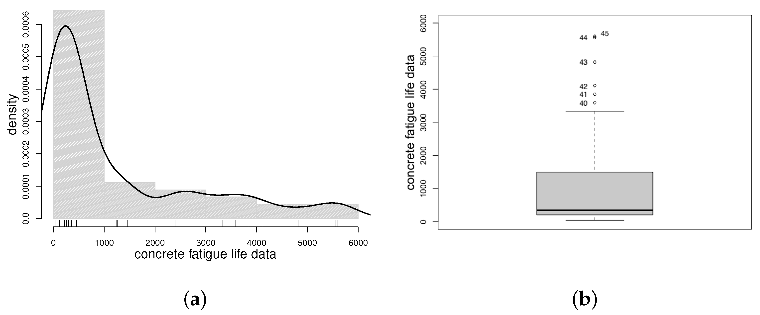
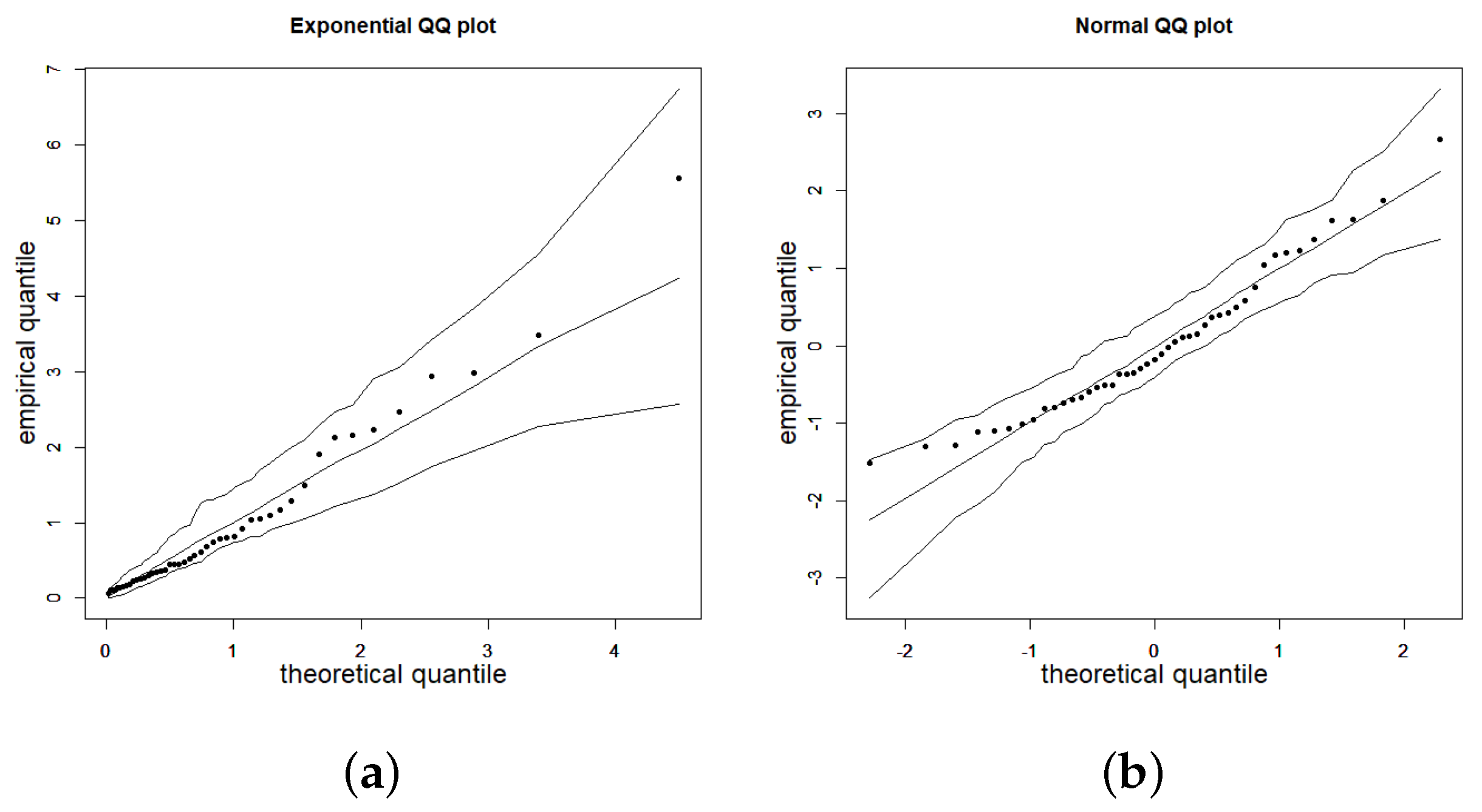
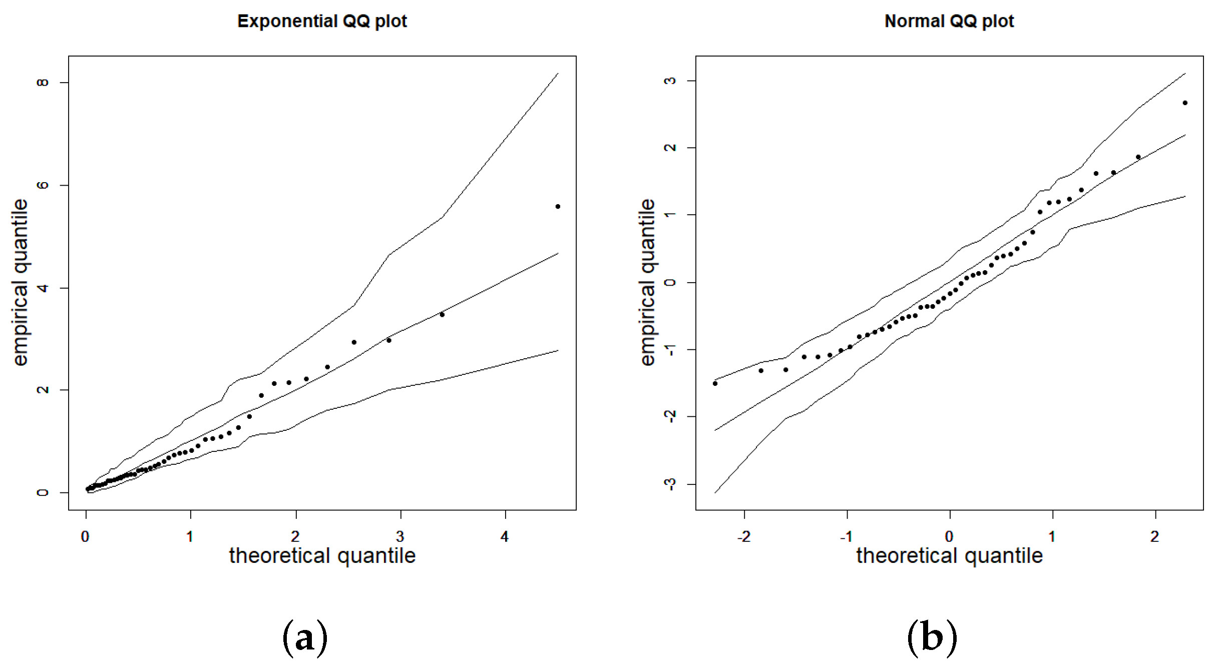
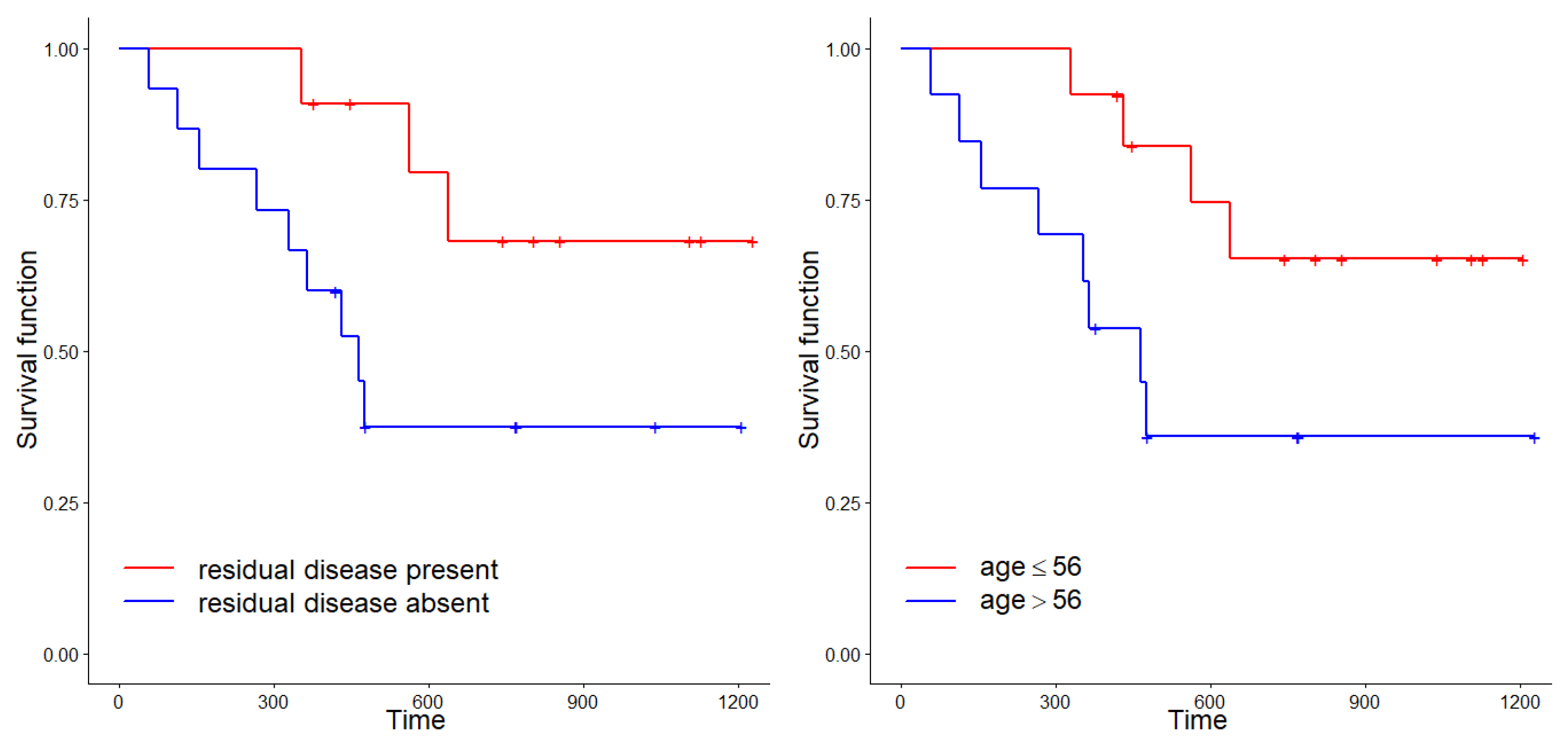
To illustrate the practical relevance of the approach, two real-world applications using authentic datasets were presented. These applications underscored the adequacy of the introduced Weibull models when data present an asymmetric distribution. Depending on which parameter is of interest in the study, one model will be more convenient to use than the other.
As part of future research, the plan is to develop an R package that facilitates inference in WEI4 and WEI5 regression models.

Author Contributions

Conceptualization, D.I.G., Y.M.G. and M.B.; methodology, D.I.G., Y.M.G. and M.B.; software, D.I.G., Y.M.G., C.M., L.S. and M.B.; validation, formal analysis, D.I.G., Y.M.G., C.M., L.S. and M.B.; investigation, D.I.G., Y.M.G., C.M., L.S. and M.B.; resources; data curation, Y.M.G. and C.M.; writing—original draft preparation, D.I.G., Y.M.G., C.M., L.S. and M.B.; writing—review and editing, D.I.G., Y.M.G., C.M., L.S. and M.B.; visualization, D.I.G., Y.M.G., C.M. and L.S. All authors have read and agreed to the published version of the manuscript.

Funding

This research received no external funding.

Data Availability Statement

Data and computational codes are available upon request from the authors.

Conflicts of Interest

The authors declare no conflicts of interest.

References

  1. Weibull, W. A statistical distribution function of wide applicability. J. Appl. Mech. 1951, 18, 293–296. [Google Scholar] [CrossRef]
  2. Keshevan, K.; Sargent, G.; Conrad, H. Statistical analysis of the Hertzian fracture of pyrex glass using the Weibull distribution function. J. Mater. Sci. 1980, 15, 839–844. [Google Scholar] [CrossRef]
  3. Queeshi, F.S.; Sheikh, A.K. Probabilistic characterization of adhesive wear in metals. IEEE Trans. Reliab. 1997, 46, 38–44. [Google Scholar]
  4. Durham, S.D.; Padgett, W.J. Cumulative damage model for system failure with application to carbon fibers and composites. Technometrics 1997, 39, 34–44. [Google Scholar] [CrossRef]
  5. Almeida, J.B. Application of Weilbull statistics to the failure of coatings. J. Mater. Process. Technol. 1999, 93, 257–263. [Google Scholar] [CrossRef]
  6. Fok, S.L.; Mitchell, B.C.; Smart, J.; Marsden, B.J. A numerical study on the application of the Weibull theory to brittle materials. Eng. Fract. Mech. 2001, 68, 1171–1179. [Google Scholar] [CrossRef]
  7. Newell, J.A.; Kurzeja, T.; Spence, M.; Lynch, M. Analysis of recoil compressive failure in high performance polymers using two-, four-parameter Weibull models. High Perform. Polym. 2002, 14, 425–434. [Google Scholar] [CrossRef]
  8. Li, Q.S.; Fang, J.Q.; Liu, D.K.; Tang, J. Failure probability prediction of concrete components. Cem. Concr. Res. 2003, 33, 1631–1636. [Google Scholar] [CrossRef]
  9. Bebbington, M.S.; Lai, C.D. On nonhomogeneous models for volcanic eruptions. Math. Geol. 1996, 28, 585–599. [Google Scholar] [CrossRef]
  10. Durrans, S.R. Low-flow analysis with a conditional Weibull tail model. Water Resour. Res. 1996, 32, 1749–1760. [Google Scholar] [CrossRef]
  11. Heo, J.H.; Boes, D.C.; Salas, J.D. Regional flood frequency analysis based on a Weibull model: Part 1. Estimation, asymptotic variances. J. Hydrol. 2001, 242, 157–170. [Google Scholar] [CrossRef]
  12. Fleming, R.A. The Weibull model and an ecological application: Describing the dynamics of foliage biomass on Scots pine. Ecol. Model. 2001, 138, 309–319. [Google Scholar] [CrossRef]
  13. Roed, K.; Zhang, T. A note on the Weibull distribution and time aggregation bias. Appl. Econ. Lett. 2002, 9, 469–472. [Google Scholar] [CrossRef]
  14. Ikki, S.S.; Ahmed, M.H. Performance of multi-hop relaying systems over Weibull fading channels. In New Technologies, Mobility and Security; Springer: Amsterdam, The Netherlands, 2007; pp. 31–38. [Google Scholar]
  15. Wang, P.; Zhang, J.; Guo, L.; Shang, T.; Cao, T.; Wang, R.; Yang, T. Performance analysis for relay-aided multihop BPPM FSO communication system over exponentiated Weibull fading channels with pointing error impairments. IEEE Photon. J. 2015, 7, 1–20. [Google Scholar] [CrossRef]
  16. Rinne, H. The Weibull Distribution: A Handbook; Chapman and Hall/CRC: New York, NY, USA, 2008. [Google Scholar]
  17. Lai, C.; Xie, M. Weibull Distributions and Their Applications. In Springer Handbook of Engineering Statistics; Pham, H., Ed.; Springer: New York, NY, USA, 2006; pp. 63–78. [Google Scholar]
  18. Lawless, J.F. Statistical Models and Methods for Lifetime Data; Wiley: New York, NY, USA, 1982. [Google Scholar]
  19. Ghitany, M.E.; Al-Hussaini, E.K.; Al-Jarallah, R.A. Marshall–Olkin extended weibull distribution and its application to censored data. J. Appl. Stat. 2005, 32, 1025–1034. [Google Scholar] [CrossRef]
  20. Klakattawi, H.S. Survival analysis of cancer patients using a new extended Weibull distribution. PLoS ONE 2022, 17, e0264229. [Google Scholar] [CrossRef]
  21. Joarder, A.; Krishna, H.; Kundu, D. Inferences on Weibull parameters with conventional type-I censoring. Comput. Stat. Data Anal. 2011, 55, 1–11. [Google Scholar] [CrossRef]
  22. Jia, X.; Wang, D.; Jiang, P.; Guo, B. Inference on the reliability of Weibull distribution with multiply Type-I censored data. Reliab. Eng. Syst. Saf. 2016, 150, 171–181. [Google Scholar] [CrossRef]
  23. Lee, C.; Famoye, F.; Olumolade, O. Beta-Weibull Distribution: Some Properties and Applications to Censored Data. J. Mod. Appl. Stat. Methods 2007, 6, 173–186. [Google Scholar] [CrossRef]
  24. Chen, M.H.; Ibrahim, J.G.; Sinha, D. A new Bayesian model for survival data with a surviving fraction. J. Am. Stat. Assoc. 1999, 94, 909–919. [Google Scholar] [CrossRef]
  25. Yin, G.; Ibrahim, J.G. Cure rate models: A unified approach. Can. J. Stat. 2005, 33, 559–570. [Google Scholar] [CrossRef]
  26. Rodrigues, J.; Cordeiro, G.M.; Cancho, V.; Balakrishnan, N. Relaxed Poisson cure rate models. Biom. J. 2016, 58, 397–415. [Google Scholar] [CrossRef] [PubMed]
  27. Gallardo, D.I.; Gómez, Y.M.; Gómez, H.W.; De Castro, M. On the use of the modified power series family of distributions in a cure rate model context. Stat. Methods Med. Res. 2020, 29, 1831–1845. [Google Scholar] [CrossRef] [PubMed]
  28. Azimi, R.; Esmailian, M.; Gallardo, D.I.; Gómez, H.J. A New Cure Rate Model Based on Flory–Schulz Distribution: Application to the Cancer Data. Mathematics 2022, 10, 4643. [Google Scholar] [CrossRef]
  29. Murthy, D.N.P.; Baik, J.; Bulmer, M.; Wilson, R.J. Two-dimensional modelling of failures. In Springer Handbook of Engineering Statistics; Pham, H., Ed.; Springer: Heidelberg/Berlin, Germany, 2004. [Google Scholar]
  30. Murthy, D.N.P.; Xie, M.; Jiang, R. Weibull Models; Wiley: New York, NY, USA, 2003. [Google Scholar]
  31. Silva, R.B.; Bourguignon, M.; Dias, C.R.B.; Cordeiro, G.M. The compound class of extended Weibull power series distributions. Comput. Stat. Data Anal. 2013, 58, 352–367. [Google Scholar] [CrossRef]
  32. Santos-Neto, M.; Bourguignon, M.; Zea, L.M.; Nascimento, A.D.C.; Cordeiro, G.M. The Marshall-Olkin extended Weibull family of distributions. J. Stat. Distrib. Appl. 2014, 1, 1–24. [Google Scholar] [CrossRef]
  33. Nascimento, A.D.C.; Bourguignon, M.; Zea, L.M.; Santos-Neto, M.; Silva, R.B.; Cordeiro, G.M. The gamma extended Weibull family of distributions. J. Stat. Theory Appl. 2014, 13, 1–16. [Google Scholar] [CrossRef]
  34. Nadarajah, S.; Kotz, S. On some recent modifications of Weibull distribution. IEEE Trans. Reliab. 2005, 54, 561–562. [Google Scholar] [CrossRef]
  35. Pham, H.; Lai, C.-D. On recent generalizations of the Weibull distribution. IEEE Trans. Reliab. 2007, 56, 454–458. [Google Scholar] [CrossRef]
  36. Almalki, S.J.; Nadarajah, S. Modifications of the Weibull distribution: A review. Reliab. Eng. Syst. Saf. 2014, 124, 32–55. [Google Scholar] [CrossRef]
  37. Wingo, D.R. The left-truncated Weibull distribution: Theory and computation. Stat. Pap. 1989, 30, 39–48. [Google Scholar] [CrossRef]
  38. Zhang, T.; Xie, M. On the upper truncated Weibull distribution and its reliability implications Reliability. Eng. Syst. Saf. 2011, 96, 194–200. [Google Scholar] [CrossRef]
  39. McEwen, R.P.; Parresol, B.R. Moment expressions and summary statistics for the complete and truncated Weibull distribution. Commun. Stat. Theory Methods 1991, 20, 1361–1372. [Google Scholar] [CrossRef]
  40. Fernandes, F.H.; Lee, H.L.; Bourguignon, M. About Shewhart control charts to monitor the Weibull mean. Qual. Reliab. Eng. Int. 2019, 35, 2343–2357. [Google Scholar] [CrossRef]
  41. Sánchez, L.; Leiva, V.; Saulo, H.; Marchant, C.; Sarabia, J. A new quantile regression model and its diagnostic analytics for a weibull distributed response with applications. Mathematics 2021, 9, 2768. [Google Scholar] [CrossRef]
  42. Yao, W.; Li, L. A New Regression Model: Modal Linear Regression. Scand. J. Stat. 2013, 41, 656–671. [Google Scholar] [CrossRef]
  43. Chen, Y.C. Modal regression using kernel density estimation: A review. WIREs Comput. Stat. 2018, 10, e1431. [Google Scholar] [CrossRef]
  44. Bourguignon, M.; Leao, J.; Gallardo, D.I. Parametric modal regression with varying precision. Biom. J. 2020, 62, 202–220. [Google Scholar] [CrossRef]
  45. Kleinbaum, D.G.; Klein, M. Survival analysis: A self-learning text. In Statistics for Biology and Health, 3rd ed.; Kleinbaum, D.G., Klein, M., Eds.; Springer: New York, NY, USA, 2012. [Google Scholar]
  46. Leiva, V. The Birnbaun-Saunders Distribution; Elsevier: Amsterdam, The Netherlands, 2016. [Google Scholar]
  47. Therneau, T.M. A Package for Survival Analysis in R. R Package Version 3.5-7, CRAN. 2023. Available online: https://CRAN.R-project.org/package=survival (accessed on 5 December 2023).
Figure 1. Histogram with the density kernel estimation (a) and boxplot (b) for the concrete fatigue life dataset.
Mathematics 12 00056 g001
Figure 2. QQ plot with the envelope of CS (a) and RQ (b) residuals for the WEI4 model.
Mathematics 12 00056 g002
Figure 3. QQ plot with the envelope of CS (a) and RQ (b) residuals for the WEI5 model.
Mathematics 12 00056 g003
Figure 4. K-M estimator for ovarian dataset separated by the residual (left panel) and age (right panel).
Mathematics 12 00056 g004
Figure 5. QQ plot with the envelope of RQ residuals for the ovarian dataset. Note that the plot is identical for WEI, WEI2, and WEI3 models.
Mathematics 12 00056 g005
Figure 6. Different measures of central tendency for the survival time in the ovarian problem in terms of age: residual = 1 (left panel) and residual = 2 (right panel). The plots are identical for WEI, WEI2, and WEI3 models.
Mathematics 12 00056 g006
Table 1. Different measures for the five parameterization of the Weibull distribution. In all parameterizations, the parameter space for ( λ , ν ) is R + 2 , except for the WEI5 model, where the parameter space is R + × ( 1 , ) .
ModelMeanModeq-QuantileVariance
WEI λ Γ 1 + 1 ν λ ( ν 1 ) ν 1 / ν , if ν > 1 0 , if ν 1 λ log ( 1 q ) 1 / ν λ 2 ω ( ν )
WEI2 λ 1 / ν Γ 1 + 1 ν ( ν 1 ) λ ν 1 / ν , if ν > 1 0 , if ν 1 log ( 1 q ) λ 1 / ν λ 2 / ν ω ( ν )
WEI3 λ λ Γ 1 + 1 ν ( ν 1 ) ν 1 / ν , if ν > 1 0 , if ν 1 λ Γ 1 + 1 ν log ( 1 q ) 1 / ν λ 2 ω ( ν ) Γ 2 1 + 1 ν
WEI4 λ Γ 1 + 1 ν log ( 1 q ) 1 / ν λ ( ν 1 ) ν [ log ( 1 q ) ] 1 / ν , if ν > 1 0 , if ν 1 λ λ 2 log 2 ( 1 q ) 2 / ν ω ( ν )
WEI5 λ 1 1 ν 1 / ν Γ 1 + 1 ν λ λ ν log ( 1 q ) ( ν 1 ) 1 / ν λ 2 1 1 ν 1 / ν ω ( ν )
NOTE: ω ( ν ) = Γ 1 + 2 ν Γ 2 1 + 1 ν .
Table 2. Function k ( λ , ν ) for the different parameterizations of the WEI model.
ModelWEIWEI2WEI3WEI4WEI5
k ( λ , ν ) λ λ 1 / ν λ [ ν { Γ ( 1 + 1 / ν ) } ν ] 1 λ log ( 1 q ) λ 1 1 ν 1 / ν
Table 3. Bias and MSE for the WEI4 model parameters, with the indicated sample size and true values of the parameters.
β 1 = 0.2;    β 2 = 1.0;    ζ 1 = 0.2;    ζ 2 = 1.0
BiasMSE
n β 1 β 2 ζ 1 ζ 2 β 1 β 2 ζ 1 ζ 2
30−0.00280.00130.07610.02320.08080.25920.23300.6466
50−0.00390.00350.03710.02960.05020.14700.09720.3091
100−0.00050.00070.01520.01790.02060.06610.04110.1357
500−0.00010.00000.0048−0.00050.00430.01340.00800.0253
β 1 = 0.2;    β 2 = 0.5;    ζ 1 = 0.2;     ζ 2 = 1.0
BiasMSE
n β 1 β 2 ζ 1 ζ 2 β 1 β 2 ζ 1 ζ 2
30−0.01530.01850.05330.05030.08430.24990.18460.5915
500.0021−0.00360.03680.03180.04300.13330.09370.3019
1000.0013−0.00100.01440.02230.02060.06190.04700.1478
500−0.00040.00010.00370.00290.00410.01340.00750.0238
β 1 = 0.5;     β 2 = 1.0;     ζ 1 = 0.2;    ζ 2 = 1.0
BiasMSE
n β 1 β 2 ζ 1 ζ 2 β 1 β 2 ζ 1 ζ 2
300.0024−0.01360.05960.05390.08670.25420.18260.5722
50−0.00470.00170.03260.02850.05150.17070.09110.3315
100−0.0004−0.00120.01840.01320.02380.07130.04030.1326
500−0.00160.00230.00200.00380.00450.01370.00780.0248
β 1 = 0.5;    β 2 = 1.5;    ζ 1 = 0.2;    ζ 2 = 1.0
BiasMSE
n β 1 β 2 ζ 1 ζ 2 β 1 β 2 ζ 1 ζ 2
300.0007−0.00670.05330.05740.08020.23630.18510.6371
50−0.00520.00210.03150.03680.04870.15290.09430.3092
100−0.00120.00160.01940.00710.02510.07140.04220.1316
5000.0006−0.00200.00400.00220.00450.01340.00760.0243
Table 4. Bias and MSE for the WEI5 model parameters, with the indicated sample size and true values of the parameters.
β 1 = 0.2;    β 2 = 1.0;    ζ 1 = 0.2;    ζ 2 = 1.0
BiasMSE
n β 1 β 2 ζ 1 ζ 2 β 1 β 2 ζ 1 ζ 2
30−0.00190.00990.01920.12260.16990.49000.08890.3378
500.0082−0.00450.01490.06200.08770.24370.04540.1648
1000.0075−0.00510.00500.03330.06590.17020.01580.0642
5000.00030.00010.00310.00220.00670.01770.00250.0110
β 1 = 0.2;    β 2 = 0.5;    ζ 1 = 0.2;     ζ 2 = 1.0
BiasMSE
n β 1 β 2 ζ 1 ζ 2 β 1 β 2 ζ 1 ζ 2
300.0043−0.00590.02110.11350.27460.51240.08650.3565
500.00210.00460.01640.06170.11460.26920.03660.1447
1000.00120.00270.00350.03960.04540.11380.01780.0673
5000.0015−0.00200.00180.00580.00670.01810.00270.0108
β 1 = 0.5;     β 2 = 1.0;     ζ 1 = 0.2;    ζ 2 = 1.0
BiasMSE
n β 1 β 2 ζ 1 ζ 2 β 1 β 2 ζ 1 ζ 2
300.0074−0.00230.01880.11260.19630.53920.08320.3169
50−0.00190.00550.01230.06380.13800.36980.04340.1694
1000.0006−0.00190.00350.03380.03600.10270.01580.0626
5000.0015−0.00200.00090.00760.00660.01750.00260.0107
β 1 = 0.5;    β 2 = 1.5;    ζ 1 = 0.2;    ζ 2 = 1.0
BiasMSE
n β 1 β 2 ζ 1 ζ 2 β 1 β 2 ζ 1 ζ 2
30−0.01360.02170.02050.11420.47251.52180.08420.3431
500.00130.00400.01040.07200.08860.26400.04140.1756
100−0.00340.00780.00560.03240.04850.13010.02260.0738
5000.0004−0.00030.00100.00630.00620.01690.00270.0108
Table 5. Mean, SD, and CSk of the CS and randomized quantile residuals for the WEI4 model, with the indicated sample size and true values of the parameters.
β 1 = 0.2;    β 2 = 1.0;    ζ 1 = 0.2;    ζ 2 = 1.0
Randomized QuantileCox–Snell
nMeanSDCSkMeanSDCSk
30−0.01761.01970.02250.98790.96861.2599
50−0.00641.00670.07610.99361.01191.8385
1000.00570.99180.15591.00241.03801.9373
5000.00850.99030.12821.00571.02561.9420
β 1 = 0.2;    β 2 = 0.5;    ζ 1 = 0.2;     ζ 2 = 1.0
randomized quantileCox–Snell
nmeanSDCSkmeanSDCSk
30−0.01240.99310.31320.98621.03881.4458
50−0.00451.0443−0.36801.00110.92071.3308
100−0.02681.0082−0.05450.97321.04822.7658
500−0.00380.98440.22640.99421.03662.0337
β 1 = 0.5;     β 2 = 1.0;     ζ 1 = 0.2;    ζ 2 = 1.0
randomized quantileCox–Snell
nmeanSDCSkmeanSDCSk
30−0.01901.0429−0.23830.99030.91261.0349
50−0.02071.0441−0.44260.98510.90501.1128
100−0.03001.0318−0.22470.98150.91641.8438
500−0.00641.0036−0.03120.99371.01552.4167
β 1 = 0.5;    β 2 = 1.5;    ζ 1 = 0.2;    ζ 2 = 1.0
randomized quantileCox–Snell
nmeanSDCSkmeanSDCSk
300.02800.99160.30171.02261.03641.2727
500.00981.0222−0.16061.01130.95571.2558
100−0.02071.0208−0.16570.98430.96071.6202
500−0.01160.99780.06710.99040.99611.9101
Table 6. Mean, SD, and CSk of the Cox–Snell and randomized quantile residuals for the WEI5 model, with the indicated sample size and true values of the parameters.
β 1 = 0.2;    β 2 = 1.0;    ζ 1 = 0.2;    ζ 2 = 1.0
Randomized QuantileCox–Snell
nMeanSDCSkMeanSDCSk
300.03190.97720.02731.00730.95871.3523
50−0.02881.01800.14520.98680.98801.1914
1000.01521.0165−0.32261.00840.94031.4739
500−0.00291.0066−0.08480.99780.98021.7448
β 1 = 0.2;    β 2 = 0.5;    ζ 1 = 0.2;     ζ 2 = 1.0
randomized quantileCox–Snell
nmeanSDCSkmeanSDCSk
300.07260.9760−0.02281.04330.94771.2336
500.01311.0012−0.09421.00430.94771.5201
100−0.02370.98670.31800.97911.04662.1566
5000.00990.98540.14561.00481.01832.0615
β 1 = 0.5;     β 2 = 1.0;     ζ 1 = 0.2;    ζ 2 = 1.0
randomized quantileCox–Snell
nmeanSDCSkmeanSDCSk
30−0.07151.0858−0.16310.97100.97731.7365
50−0.01931.0235−0.02000.99140.97121.6429
100−0.01151.0165−0.05160.99600.95901.4681
500−0.01271.0102−0.03330.99300.99061.8522
β 1  = 0.5;    β 2 = 1.5;    ζ 1 = 0.2;    ζ 2 = 1.0
randomized quantileCox–Snell
nmeanSDCSkmeanSDCSk
300.01971.0379−0.42231.01330.92511.3285
500.01561.01190.02201.01561.03442.2866
1000.00321.0122−0.17201.00230.91951.1461
5000.00311.0092−0.11791.00440.95771.5290
Table 7. Descriptive statistics of the concrete fatigue life dataset.
nminMaxMeanMedianSDCSkCVCK
453755981216.583421598.601.41131.400.77
Table 8. ML estimates, SEs, p-values, AIC, and KS p-value of the indicated model.
WEI4WEI5
ParameterEstimateSEp-ValueEstimateSEp-Value
λ β 1 29.28051.4737<0.000129.59631.8853<0.0001
β 2 −25.81661.6582<0.0001−26.31322.1276<0.0001
ν ζ 1 1.47022.21390.50661.53621.81170.3965
ζ 2 −0.79992.47530.7466−0.87402.02180.6655
AIC 635.03635.02
KS p-value 0.8729 (CS)0.4339 (RQ)0.8753 (CS)0.4102 (RQ)
AD p-value 0.1082 (RQ)0.1117 (RQ)
CVM p-value 0.1203 (RQ)0.1234 (RQ)
Table 9. The AIC for the fitted model ovarian dataset.
CovariatesModel
λ ν WEIWEI2WEI3
Only interceptOnly intercept199.91
Residual plus ageOnly intercept186.04
Residual plus ageResidual plus age189.56190.04189.53
Table 10. ML estimate, standard error (SE) for WEI2, considering the residual plus age covariates for the ovarian dataset.
WEI2
ParametersEstimateSE
Intercept−20.53741.1339
λ residual0.97200.4152
age0.14010.0207
ν Intercept0.55590.0155
AIC 186.04
KS p-value 0.6703
AD p-value 0.1916
CVM p-value 0.1895
Disclaimer/Publisher’s Note: The statements, opinions and data contained in all publications are solely those of the individual author(s) and contributor(s) and not of MDPI and/or the editor(s). MDPI and/or the editor(s) disclaim responsibility for any injury to people or property resulting from any ideas, methods, instructions or products referred to in the content.

