


Extropy and Some of Its More Recent Related Measures for Concomitants of K-Record Values in an Extended FGM Family

 ,
,  , and
, and
Abstract
:1. Introduction
Motivations of the Work
2. CKRV Based on EFGM(c,d) and EX, with Some of Its Associated Measures
2.1. The Marginal Distribution of CKRV Based on EFGM(c,d)
2.2. EX and Some of Its More Recent Related Measures
2.2.1. EX of CKRV for EFGM(c,d)
2.2.2. NCREX of CKRV for EFGM(c,d)
2.2.3. WNCREX of CKRV for EFGM(c,d)
- Putting (i.e., ) in EFGM-EWF, we obtain EFGM with Rayleigh distribution marginals (denoted by EFGM-RD), which is given byTherefore, the WNCREX of would be
- Choosing (i.e., ), in EFGM- EWF, we obtain EFGM with Pareto type-I distribution marginals (denoted by EFGM-PID), as followsFurther, by using (27), we have
- 1.
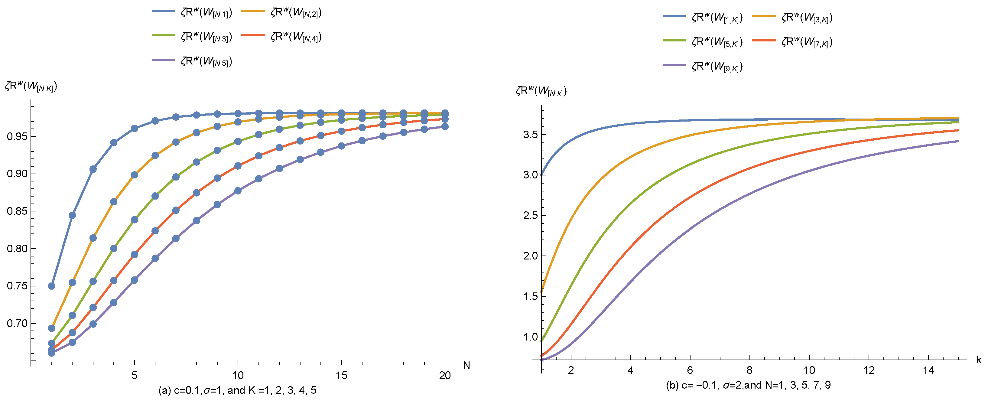
- With fixed N, and the value of increases as K decreases (see Figure 1a) and stability occurs for large
- 2.
- For the fixed large the value of increases with the increasing N; see Figure 1b.
- 1.
- Stability occurs for large N and see Figure 2a,b.
- 2.
- With fixed c and the values of are very near to each other as N and K rise.
2.2.4. NCEX of CKRV for EFGM(c,d)
2.2.5. WNCEX of CKRV for EFGM(c,d)
3. Numerical Study for the EX, NCREX, WNCREX, NCEX, and WNCEX
- The value of at
- For large K (), and the value of increases as the value of N increases.
- For large K (), and the value of decreases as the value of N increases.
- For and large K (), the value of increases as the value of N increases along with the values of parameters as and
- For and large K (), the value of decreases as the value of N increases along with the values of parameters as , , , , and
4. Non-Parametric Estimation of NCREX, WNCREX, NCEX, and WNCEX
4.1. EM of NCREX in CKRV Based on EFGM(c,d)
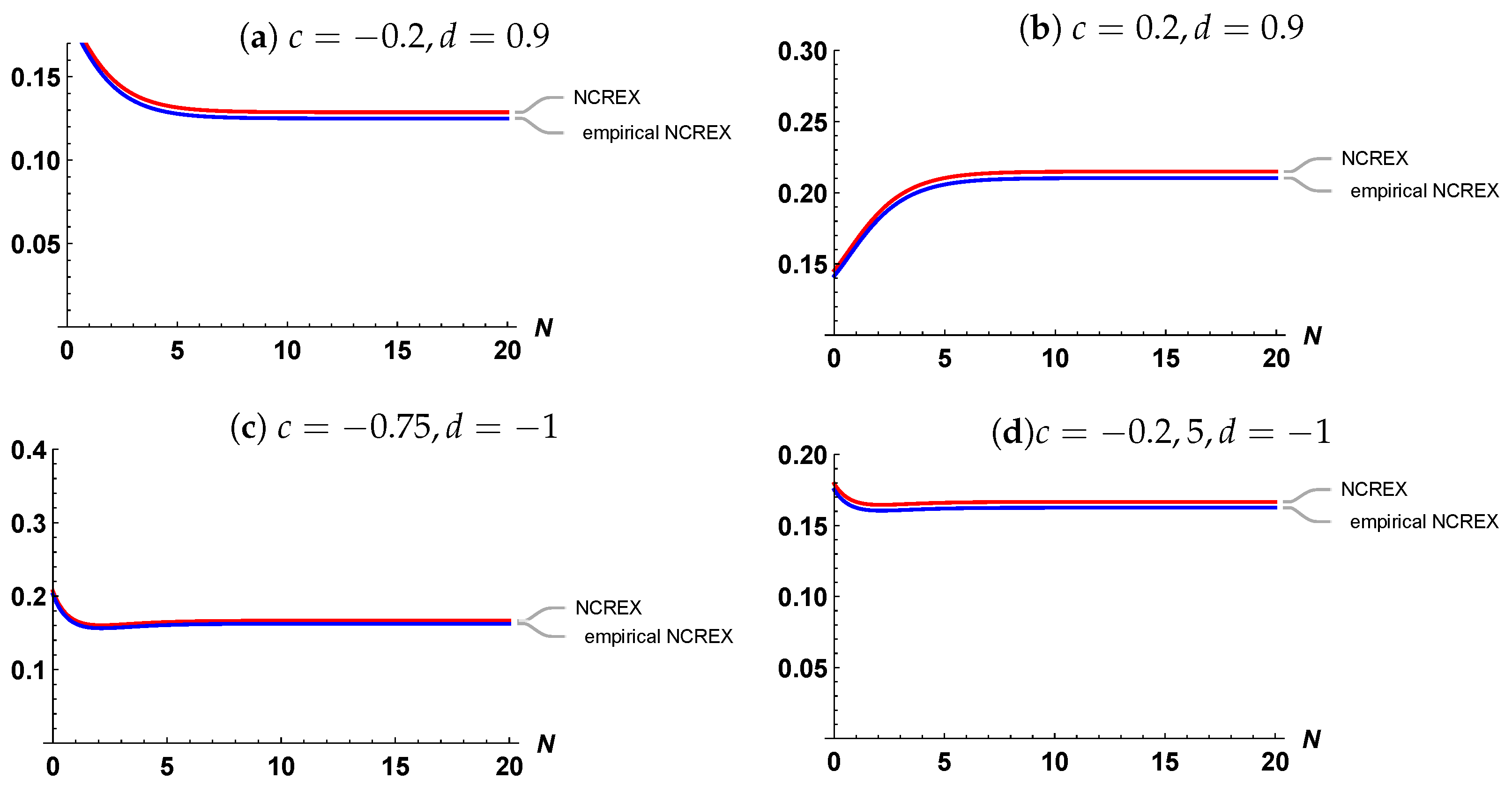
- With fixed N and and increase as c increases.
- With fixed N and and increase as increases.

| N | |||||||||
|---|---|---|---|---|---|---|---|---|---|
| 3 | 0.5 | 0.102492 | 0.107408 | 0.117768 | 0.123213 | 0.001551 | 0.001662 | 0.001911 | 0.002051 |
| 3 | 1 | 0.204985 | 0.214816 | 0.235537 | 0.246426 | 0.006204 | 0.006646 | 0.007643 | 0.008204 |
| 3 | 2 | 0.409970 | 0.429632 | 0.471073 | 0.492852 | 0.024818 | 0.026585 | 0.030574 | 0.032817 |
| 5 | 0.5 | 0.092915 | 0.102344 | 0.123384 | 0.134995 | 0.001350 | 0.001548 | 0.002056 | 0.002377 |
| 5 | 1 | 0.185829 | 0.204687 | 0.246767 | 0.269990 | 0.005400 | 0.006191 | 0.008222 | 0.009507 |
| 5 | 2 | 0.371659 | 0.409375 | 0.493535 | 0.539980 | 0.021598 | 0.024766 | 0.032889 | 0.038028 |
| 8 | 0.5 | 0.087208 | 0.099217 | 0.127056 | 0.142886 | 0.001238 | 0.001480 | 0.002154 | 0.002612 |
| 8 | 1 | 0.174415 | 0.198434 | 0.254113 | 0.285773 | 0.004954 | 0.005921 | 0.008616 | 0.010449 |
| 8 | 2 | 0.348831 | 0.396868 | 0.508226 | 0.571545 | 0.019815 | 0.023684 | 0.034463 | 0.041796 |
| 10 | 0.5 | 0.085830 | 0.098448 | 0.127985 | 0.144904 | 0.001212 | 0.001464 | 0.002179 | 0.002675 |
| 10 | 1 | 0.171660 | 0.196897 | 0.255971 | 0.289808 | 0.004850 | 0.005856 | 0.008717 | 0.010699 |
| 10 | 2 | 0.343320 | 0.393793 | 0.511941 | 0.579617 | 0.019399 | 0.023423 | 0.034869 | 0.042796 |
4.2. EM of WNCREX in CKRV Based on EFGM(c,d)
- Generally, with fixed N and and increase with increasing
- Generally, with fixed N and and increase with increasing .
| N | |||||||||
|---|---|---|---|---|---|---|---|---|---|
| 3 | 0.5 | 0.051246 | 0.053704 | 0.058884 | 0.061607 | 0.000388 | 0.000415 | 0.000478 | 0.000513 |
| 3 | 1 | 0.102492 | 0.107408 | 0.117768 | 0.123213 | 0.001551 | 0.001662 | 0.001911 | 0.002051 |
| 3 | 2 | 0.204985 | 0.214816 | 0.235537 | 0.246426 | 0.006204 | 0.006646 | 0.007643 | 0.008204 |
| 5 | 0.5 | 0.046457 | 0.051172 | 0.061692 | 0.067497 | 0.000337 | 0.000387 | 0.000514 | 0.000594 |
| 5 | 1 | 0.092915 | 0.102344 | 0.123384 | 0.134995 | 0.001350 | 0.001548 | 0.002056 | 0.002377 |
| 5 | 2 | 0.185829 | 0.204687 | 0.246767 | 0.269990 | 0.005400 | 0.006191 | 0.008222 | 0.009507 |
| 8 | 0.5 | 0.043604 | 0.049609 | 0.063528 | 0.071443 | 0.000310 | 0.000370 | 0.000538 | 0.000653 |
| 8 | 1 | 0.087208 | 0.099217 | 0.127056 | 0.142886 | 0.001238 | 0.001480 | 0.002154 | 0.002612 |
| 8 | 2 | 0.174415 | 0.198434 | 0.254113 | 0.285773 | 0.004954 | 0.005921 | 0.008616 | 0.010449 |
| 10 | 0.5 | 0.042915 | 0.049224 | 0.063993 | 0.072452 | 0.000303 | 0.000366 | 0.000545 | 0.000669 |
| 10 | 1 | 0.085830 | 0.098448 | 0.127985 | 0.144904 | 0.001212 | 0.001464 | 0.002179 | 0.002675 |
| 10 | 2 | 0.171660 | 0.196897 | 0.255971 | 0.289808 | 0.004850 | 0.005856 | 0.008717 | 0.010699 |
4.3. EM of NCEX in CKRV Based on EFGM(c,d)
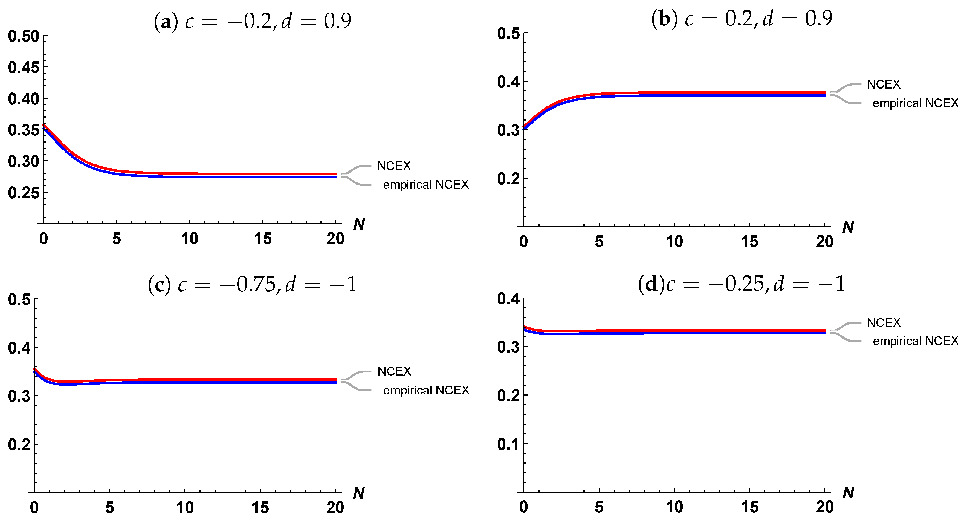
- At fixed N and and increase as the value of c increases.
- At fixed N and and increase as the value of increases.
| N | |||||||||
|---|---|---|---|---|---|---|---|---|---|
| 3 | 0.5 | 0.317745 | 0.327711 | 0.347113 | 0.356549 | 0.011409 | 0.012208 | 0.013878 | 0.014747 |
| 3 | 1 | 0.635491 | 0.655422 | 0.694226 | 0.713098 | 0.045635 | 0.048830 | 0.055513 | 0.058989 |
| 3 | 2 | 1.270980 | 1.310840 | 1.388450 | 1.426200 | 0.182540 | 0.195321 | 0.222053 | 0.235954 |
| 5 | 0.5 | 0.296643 | 0.317435 | 0.356837 | 0.375448 | 0.009847 | 0.011385 | 0.014774 | 0.016601 |
| 5 | 1 | 0.593286 | 0.634870 | 0.713675 | 0.750895 | 0.039389 | 0.045538 | 0.059097 | 0.066403 |
| 5 | 2 | 1.186570 | 1.269740 | 1.427350 | 1.501790 | 0.157557 | 0.182153 | 0.236388 | 0.265614 |
| 8 | 0.5 | 0.282818 | 0.310796 | 0.362931 | 0.387088 | 0.008918 | 0.010875 | 0.015356 | 0.017820 |
| 8 | 1 | 0.565635 | 0.621591 | 0.725862 | 0.774177 | 0.035674 | 0.043501 | 0.061424 | 0.071280 |
| 8 | 2 | 1.131270 | 1.243180 | 1.451720 | 1.548350 | 0.142696 | 0.174003 | 0.245696 | 0.285121 |
| 10 | 0.5 | 0.279318 | 0.309126 | 0.364441 | 0.389948 | 0.008695 | 0.010750 | 0.015503 | 0.018129 |
| 10 | 1 | 0.558636 | 0.618252 | 0.728881 | 0.779895 | 0.034780 | 0.042999 | 0.062010 | 0.072515 |
| 10 | 2 | 1.117270 | 1.236500 | 1.457760 | 1.559790 | 0.139120 | 0.171997 | 0.248041 | 0.290061 |
4.4. EM of WNCEX in CKRV Based on EFGM(c,d)
- For fixed N and and increase as c increases.
- For fixed N and and increase as increases.
| N | |||||||||
|---|---|---|---|---|---|---|---|---|---|
| 3 | 0.5 | 0.158873 | 0.163855 | 0.173556 | 0.178275 | 0.002852 | 0.003052 | 0.003470 | 0.003687 |
| 3 | 1 | 0.317745 | 0.327711 | 0.347113 | 0.356549 | 0.011409 | 0.012208 | 0.013878 | 0.014747 |
| 3 | 2 | 0.635491 | 0.655422 | 0.694226 | 0.713098 | 0.045635 | 0.048830 | 0.055513 | 0.058989 |
| 5 | 0.5 | 0.148321 | 0.158718 | 0.178419 | 0.187724 | 0.002462 | 0.002846 | 0.003694 | 0.004150 |
| 5 | 1 | 0.296643 | 0.317435 | 0.356837 | 0.375448 | 0.009847 | 0.011385 | 0.014774 | 0.016601 |
| 5 | 2 | 0.593286 | 0.634870 | 0.713675 | 0.750895 | 0.039389 | 0.045538 | 0.059097 | 0.066403 |
| 8 | 0.5 | 0.141409 | 0.155398 | 0.181465 | 0.193544 | 0.002230 | 0.002719 | 0.003839 | 0.004455 |
| 8 | 1 | 0.282818 | 0.310796 | 0.362931 | 0.387088 | 0.008918 | 0.010875 | 0.015356 | 0.017820 |
| 8 | 2 | 0.565635 | 0.621591 | 0.725862 | 0.774177 | 0.035674 | 0.043501 | 0.061424 | 0.071280 |
| 10 | 0.5 | 0.139659 | 0.154563 | 0.182220 | 0.194974 | 0.002174 | 0.002687 | 0.003876 | 0.004532 |
| 10 | 1 | 0.279318 | 0.309126 | 0.364441 | 0.389948 | 0.008695 | 0.010750 | 0.015503 | 0.018129 |
| 10 | 2 | 0.558636 | 0.618252 | 0.728881 | 0.779895 | 0.034780 | 0.042999 | 0.062010 | 0.072515 |
5. Conclusions
Author Contributions
Funding
Data Availability Statement
Acknowledgments
Conflicts of Interest
Abbreviations
| RVs | random variables |
| CDF | cumulative distribution function |
| probability density function | |
| QF | quantile function |
| FGM | Farlie–Gumbel–Morgenstern |
| EFGM | extended Farlie–Gumbel–Morgenstern |
| OSs | order statistics |
| KRVs | K-record upper values |
| EX | extropy |
| CREX | cumulative residual extropy |
| CKRV | K-record upper values |
| NCREX | negative cumulative residual extropy |
| WNCREX | weighted negative cumulative residual extropy |
| NCEX | negative cumulative extropy |
| WNCEX | weighted negative cumulative extropy |
| EFGM-UD | EFGM family with uniform marginals |
| EFGM-ED | EFGM family with exponential marginals |
| EFGM-PFD | EFGM family with power function distribution marginals |
| EFGM-PID | EFGM family with Pareto type-I distribution marginals |
References
- Ghosh, S.; Sheppard, L.W.; Holder, M.T.; Loecke, T.D.; Reid, P.C.; Bever, J.D.; Reuman, D.C. Copulas and their potential for ecology. Adv. Ecol. Res. 2020, 62, 409–468. [Google Scholar]
- Shrahili, M.; Alotaibi, N. A new parametric life family of distributions: Properties, copula and modeling failure and service times. Symmetry 2020, 12, 1462. [Google Scholar] [CrossRef]
- Ebaid, R.; Elbadawy, W.; Ahmed, E.; Abdelghaly, A. A new extension of the FGM copula with an application in reliability. Comm. Statist. Theory Meth. 2022, 51, 2953–2961. [Google Scholar] [CrossRef]
- Barakat, H.M.; Alawady, M.A.; Husseiny, I.A.; Abd Elgawad, M.A. A more flexible counterpart of a Huang-Kotz’s copula-type. Comptes Rendus Acad. Bulg. Sci. 2022, 75, 952–958. [Google Scholar] [CrossRef]
- Bairamov, I. New generalized Farlie-Gumbel-Morgenstern distributions and concomitants of order statistics. J. Appl. Statist. 2001, 28, 521–536. [Google Scholar] [CrossRef]
- Mohamed, M.S. On concomitants of ordered random variables under general forms of Morgenstern family. Filomat 2019, 33, 2771–2780. [Google Scholar] [CrossRef]
- Barakat, H.M.; Husseiny, I.A. Some information measures in concomitants of generalized order statistics under iterated Farlie-Gumbel-Morgenstern bivariate type. Quaest. Math. 2021, 44, 581–598. [Google Scholar] [CrossRef]
- Abd Elgawad, M.A.; Barakat, H.M.; Abd El-Rahman, D.A.; Alyami, S.A. Scrutiny of a more flexible counterpart of Huang-Kotz-FGM-distributions in the perspective of some information measures. Symmetry 2023, 15, 1257. [Google Scholar] [CrossRef]
- Dziubdziela, W.; Kopociński, B. Limiting properties of the k-th record values. Appl. Math. 1976, 2, 187–190. [Google Scholar] [CrossRef]
- Aly, A.E. Prediction of the exponential fractional upper record-values. Math. Slovaca 2022, 72, 491–506. [Google Scholar] [CrossRef]
- Alawady, M.A.; Barakat, H.M.; Mansour, G.M.; Husseiny, I.A. Information measures and concomitants of k-record values based on Sarmanov family of bivariate distributions. Bull. Malays. Math. Sci. Soc. 2023, 46, 9. [Google Scholar] [CrossRef]
- Berred, M. K-record values and the extreme-value index. J. Stat. Plann. Inf. 1995, 45, 49–63. [Google Scholar] [CrossRef]
- Fashandi, M.; Ahmadi, J. Characterizations of symmetric distributions based on Renyi entropy. Statist. Probab. Lett. 2012, 82, 798–804. [Google Scholar] [CrossRef]
- Bdair, O.M.; Raqab, M.Z. Mean residual life of kth records under double monitoring. Bull. Malays. Math. Sci. Soc. 2014, 37, 457–464. [Google Scholar]
- Chacko, M.; Shy Mary, M. Concomitants of k-record values arising from Morgenstern family of distributions and their applications in parameter estimation. Stat. Papers 2013, 54, 21–46. [Google Scholar] [CrossRef]
- Chacko, M.; Muraleedharan, L. Inference based on k-record values from generalized exponential distribution. Statistica 2018, 78, 37–56. [Google Scholar]
- Thomas, P.Y.; Anne, P.; Veena, T.G. Characterization of bivariate distributions using concomitants of generalized (k) record values. Statistica 2014, 74, 431–446. [Google Scholar]
- Lad, F.; Sanfilippo, G.; Agro, G. Extropy: Complementary dual of entropy. Stat. Sci. 2015, 30, 40–58. [Google Scholar] [CrossRef]
- Husseiny, I.A.; Barakat, H.M.; Mansour, G.M.; Alawady, M.A. Information measures in records and their concomitants arising from Sarmanov family of bivariate distributions. J. Comp. Appl. Math. 2022, 408, 114120. [Google Scholar] [CrossRef]
- Qiu, G. The extropy of order statistics and record values. Stat. Probab. Lett. 2017, 120, 52–60. [Google Scholar] [CrossRef]
- Qiu, G.; Jia, K. The residual extropy of order statistics. Stat. Probab. Lett. 2018, 133, 15–22. [Google Scholar] [CrossRef]
- Irshad, M.R.; Archana, K.; Al-Omari, A.I.; Maya, R.; Alomani, G. Extropy based on concomitants of order statistics in Farlie-Gumbel-Morgenstern Family for random variables representing past life. Axioms 2023, 12, 792. [Google Scholar] [CrossRef]
- Almaspoor, Z.; Tahmasebi, S.; Jafari, A.A. Measures of extropy for concomitants of generalized order statistics in Morgenstern family. J. Stat. Theory Appl. 2021, 21, 1–20. [Google Scholar] [CrossRef]
- Husseiny, I.A.; Syam, A.H. The extropy of concomitants of generalized order statistics from Huang-Kotz-Morgenstern bivariate distribution. J. Math. 2022, 6385998. [Google Scholar] [CrossRef]
- Husseiny, I.A.; Alawady, M.A.; Alyami, S.A.; Abd Elgawad, M.A. Measures of extropy based on concomitants of generalized order statistics under a general framework from iterated morgenstern family. Mathematics 2023, 11, 1377. [Google Scholar] [CrossRef]
- Jahanshahi, S.; Zarei, H.; Khammar, A. On cumulative residual extropy. Probab. Eng. Inf. Sci. 2020, 34, 605–625. [Google Scholar] [CrossRef]
- Hashempour, M.; Kazemi, M.R.; Tahmasebi, S. On weighted cumulative residual extropy: Characterization, estimation and testing. Statistics 2022, 56, 681–698. [Google Scholar] [CrossRef]
- Tahmasebi, S.; Toomaj, A. On negative cumulative extropy with applications. Commun. Stat. Theory Methods 2021, 51, 5025–5047. [Google Scholar] [CrossRef]
- Chaudhary, K.S.; Gupta, N.; Kumar Sahu, P. On general weighted cumulative residual extropy and general weighted negative cumulative extropy. Statistics 2023, 57, 1117–1141. [Google Scholar] [CrossRef]
- Jafari, A.A.; Almaspoor, Z.; Tahmasebi, S. General results on bivariate extended Weibull Morgenstern family and concomitants of its generalized order statistics. Ric. Mat. 2021, 1–22. [Google Scholar] [CrossRef]
- Chakraborty, S.; Das, O.; Pradhan, B. Weighted negative cumulative extropy with application in testing uniformity. Phys. A Stat. Mech. Appl. 2023, 624, 128957. [Google Scholar] [CrossRef]

| 2 | 1 | −0.500296 | −0.500296 | −0.501042 | −0.500116 | −0.503464 | −0.503464 | −0.503407 | −0.503407 |
| 2 | 3 | −0.500280 | −0.500280 | −0.501775 | −0.500197 | −0.504957 | −0.504957 | −0.504749 | −0.504749 |
| 2 | 5 | −0.509920 | −0.509920 | −0.501079 | −0.500120 | −0.523053 | −0.523053 | −0.526828 | −0.526828 |
| 2 | 7 | −0.523524 | −0.523524 | −0.500329 | −0.500037 | −0.537641 | −0.537641 | −0.546456 | −0.546456 |
| 6 | 1 | −0.500340 | −0.500340 | −0.510762 | −0.501196 | −0.511352 | −0.511352 | −0.508801 | −0.508801 |
| 6 | 3 | −0.502672 | −0.502672 | −0.500001 | −0.500000 | −0.503523 | −0.503523 | −0.504500 | −0.504500 |
| 6 | 5 | −0.502570 | −0.502570 | −0.501708 | −0.500190 | −0.500037 | −0.500037 | −0.500315 | −0.500315 |
| 6 | 7 | −0.500417 | −0.500417 | −0.502927 | −0.500325 | −0.501888 | −0.501888 | −0.501237 | −0.501237 |
| 40 | 1 | −0.507091 | −0.507091 | −0.530776 | −0.503420 | −0.514590 | −0.514590 | −0.508321 | −0.508321 |
| 40 | 3 | −0.502546 | −0.502546 | −0.520221 | −0.502247 | −0.513887 | −0.513887 | −0.509327 | −0.509327 |
| 40 | 5 | −0.500485 | −0.500485 | −0.512740 | −0.501416 | −0.512936 | −0.512936 | −0.509918 | −0.509918 |
| 40 | 7 | −0.500003 | −0.500003 | −0.507577 | −0.500842 | −0.511804 | −0.511804 | −0.510114 | −0.510114 |
| 100 | 1 | −0.509078 | −0.509078 | −0.534630 | −0.503848 | −0.514752 | −0.514752 | −0.507955 | −0.507955 |
| 100 | 3 | −0.506407 | −0.506407 | −0.529423 | −0.503269 | −0.514562 | −0.514562 | −0.508484 | −0.508484 |
| 100 | 5 | −0.504327 | −0.504327 | −0.524863 | −0.502763 | −0.514319 | −0.514319 | −0.508947 | −0.508947 |
| 100 | 7 | −0.502751 | −0.502751 | −0.520883 | −0.502320 | −0.514028 | −0.514028 | −0.509341 | −0.509341 |
| 2 | 1 | −0.123657 | −0.126435 | −0.120182 | −0.123307 | −0.113982 | −0.137343 | −0.114444 | −0.136667 |
| 2 | 3 | −0.126394 | −0.123693 | −0.132466 | −0.127341 | −0.139923 | −0.111974 | −0.138892 | −0.112657 |
| 2 | 5 | −0.134587 | −0.118514 | −0.130705 | −0.126812 | −0.159545 | −0.099277 | −0.160551 | −0.098197 |
| 2 | 7 | −0.141051 | −0.116300 | −0.128049 | −0.125989 | −0.170707 | −0.093696 | −0.173601 | −0.091548 |
| 6 | 1 | −0.126541 | −0.123565 | −0.112295 | −0.119868 | −0.106026 | −0.148318 | −0.108578 | −0.144292 |
| 6 | 3 | −0.121247 | −0.129588 | −0.124808 | −0.124936 | −0.113894 | −0.137455 | −0.112965 | −0.138502 |
| 6 | 5 | −0.121311 | −0.129492 | −0.132310 | −0.127294 | −0.123794 | −0.126220 | −0.121671 | −0.128432 |
| 6 | 7 | −0.123417 | −0.126714 | −0.134828 | −0.128032 | −0.133986 | −0.116737 | −0.131897 | −0.118506 |
| 40 | 1 | −0.132902 | −0.119314 | −0.108231 | −0.116846 | −0.103818 | −0.151764 | −0.108993 | −0.143720 |
| 40 | 3 | −0.129469 | −0.121327 | −0.109635 | −0.118193 | −0.104269 | −0.151045 | −0.108138 | −0.144903 |
| 40 | 5 | −0.126852 | −0.123299 | −0.111563 | −0.119459 | −0.104902 | −0.150048 | −0.107661 | −0.145573 |
| 40 | 7 | −0.124863 | −0.125138 | −0.113794 | −0.120633 | −0.105696 | −0.148821 | −0.107506 | −0.145792 |
| 100 | 1 | −0.134106 | −0.118731 | −0.107956 | −0.116433 | −0.103716 | −0.151929 | −0.109320 | −0.143274 |
| 100 | 3 | −0.132459 | −0.119543 | −0.108353 | −0.116999 | −0.103836 | −0.151736 | −0.108851 | −0.143916 |
| 100 | 5 | −0.130984 | −0.120368 | −0.108878 | −0.117554 | −0.103990 | −0.151489 | −0.108454 | −0.144463 |
| 100 | 7 | −0.129662 | −0.121198 | −0.109511 | −0.118097 | −0.104177 | −0.151191 | −0.108126 | −0.144920 |
| 2 | 1 | 0.167233 | 0.166122 | 0.172991 | 0.168758 | 0.177954 | 0.156043 | 0.176974 | 0.156974 |
| 2 | 3 | 0.166137 | 0.167217 | 0.158634 | 0.163961 | 0.154035 | 0.180249 | 0.155289 | 0.178900 |
| 2 | 5 | 0.163806 | 0.170236 | 0.160383 | 0.164555 | 0.140612 | 0.197140 | 0.141023 | 0.197142 |
| 2 | 7 | 0.162557 | 0.172457 | 0.163179 | 0.165499 | 0.134158 | 0.206390 | 0.133927 | 0.207775 |
| 6 | 1 | 0.166084 | 0.167274 | 0.187525 | 0.173449 | 0.187588 | 0.147921 | 0.183531 | 0.151388 |
| 6 | 3 | 0.168430 | 0.165094 | 0.166897 | 0.166744 | 0.178054 | 0.155955 | 0.178564 | 0.155580 |
| 6 | 5 | 0.168395 | 0.165122 | 0.158786 | 0.164013 | 0.167808 | 0.165532 | 0.169737 | 0.163653 |
| 6 | 7 | 0.167341 | 0.166022 | 0.156399 | 0.163198 | 0.158759 | 0.174937 | 0.160752 | 0.172804 |
| 40 | 1 | 0.164202 | 0.169638 | 0.202837 | 0.178235 | 0.190550 | 0.145580 | 0.183043 | 0.151789 |
| 40 | 3 | 0.165129 | 0.168386 | 0.195648 | 0.176006 | 0.189934 | 0.146061 | 0.184051 | 0.150962 |
| 40 | 5 | 0.165973 | 0.167395 | 0.189434 | 0.174054 | 0.189079 | 0.146734 | 0.184621 | 0.150499 |
| 40 | 7 | 0.166722 | 0.166612 | 0.184065 | 0.172346 | 0.188022 | 0.147574 | 0.184806 | 0.150349 |
| 100 | 1 | 0.163916 | 0.170066 | 0.205177 | 0.178954 | 0.190690 | 0.145471 | 0.182663 | 0.152104 |
| 100 | 3 | 0.164312 | 0.169479 | 0.201985 | 0.177973 | 0.190526 | 0.145599 | 0.183210 | 0.151651 |
| 100 | 5 | 0.164698 | 0.168944 | 0.198977 | 0.177042 | 0.190314 | 0.145764 | 0.183677 | 0.151268 |
| 100 | 7 | 0.165072 | 0.168458 | 0.196142 | 0.176160 | 0.190059 | 0.145963 | 0.184065 | 0.150951 |
| 2 | 1 | 0.505648 | 0.494537 | 0.521094 | 0.506973 | 0.548594 | 0.455150 | 0.546296 | 0.457407 |
| 2 | 3 | 0.494686 | 0.505489 | 0.473245 | 0.490983 | 0.446783 | 0.558576 | 0.450112 | 0.555050 |
| 2 | 5 | 0.470954 | 0.535246 | 0.479067 | 0.492962 | 0.391923 | 0.632996 | 0.389872 | 0.639289 |
| 2 | 7 | 0.457850 | 0.556852 | 0.488380 | 0.496108 | 0.366321 | 0.674366 | 0.361141 | 0.689354 |
| 6 | 1 | 0.494154 | 0.506059 | 0.569655 | 0.522620 | 0.590719 | 0.421552 | 0.576212 | 0.433355 |
| 6 | 3 | 0.517518 | 0.484152 | 0.500769 | 0.500256 | 0.549026 | 0.454782 | 0.553521 | 0.451371 |
| 6 | 5 | 0.517167 | 0.484440 | 0.473750 | 0.491155 | 0.504873 | 0.495168 | 0.513692 | 0.486650 |
| 6 | 7 | 0.506724 | 0.493537 | 0.465809 | 0.488440 | 0.466523 | 0.535518 | 0.473890 | 0.527455 |
| 40 | 1 | 0.475038 | 0.529394 | 0.620934 | 0.538602 | 0.603777 | 0.411993 | 0.573977 | 0.435068 |
| 40 | 3 | 0.484511 | 0.517080 | 0.596844 | 0.531158 | 0.601059 | 0.413952 | 0.578600 | 0.431538 |
| 40 | 5 | 0.493045 | 0.507258 | 0.576044 | 0.524640 | 0.597284 | 0.416699 | 0.581216 | 0.429564 |
| 40 | 7 | 0.500552 | 0.499450 | 0.558084 | 0.518940 | 0.592630 | 0.420129 | 0.582068 | 0.428926 |
| 100 | 1 | 0.472086 | 0.533588 | 0.628780 | 0.541003 | 0.604398 | 0.411549 | 0.572233 | 0.436414 |
| 100 | 3 | 0.476169 | 0.527835 | 0.618079 | 0.537725 | 0.603670 | 0.412070 | 0.574742 | 0.434480 |
| 100 | 5 | 0.480122 | 0.522583 | 0.607998 | 0.534618 | 0.602737 | 0.412741 | 0.576881 | 0.432844 |
| 100 | 7 | 0.483931 | 0.517788 | 0.598501 | 0.531674 | 0.601610 | 0.413553 | 0.578665 | 0.431489 |
| 2 | 1 | 0.042230 | 0.041118 | 0.043778 | 0.042364 | 0.046519 | 0.037175 | 0.046286 | 0.037397 |
| 2 | 3 | 0.041133 | 0.042214 | 0.038994 | 0.040765 | 0.036335 | 0.047515 | 0.036663 | 0.047157 |
| 2 | 5 | 0.038696 | 0.045125 | 0.039575 | 0.040963 | 0.030814 | 0.054922 | 0.030571 | 0.055512 |
| 2 | 7 | 0.037294 | 0.047194 | 0.040505 | 0.041278 | 0.028226 | 0.059030 | 0.027637 | 0.060458 |
| 6 | 1 | 0.041080 | 0.042270 | 0.048651 | 0.043931 | 0.050717 | 0.033800 | 0.049261 | 0.034975 |
| 6 | 3 | 0.043401 | 0.040064 | 0.041744 | 0.041692 | 0.046563 | 0.037138 | 0.047005 | 0.036790 |
| 6 | 5 | 0.043366 | 0.040093 | 0.039045 | 0.040783 | 0.042154 | 0.041183 | 0.043035 | 0.040331 |
| 6 | 7 | 0.042336 | 0.041018 | 0.038253 | 0.040511 | 0.038315 | 0.045215 | 0.039052 | 0.044408 |
| 40 | 1 | 0.039123 | 0.044559 | 0.053815 | 0.045533 | 0.052016 | 0.032838 | 0.049039 | 0.035148 |
| 40 | 3 | 0.040101 | 0.043358 | 0.051387 | 0.044787 | 0.051746 | 0.033035 | 0.049498 | 0.034792 |
| 40 | 5 | 0.040968 | 0.042389 | 0.049294 | 0.044133 | 0.051370 | 0.033312 | 0.049758 | 0.034592 |
| 40 | 7 | 0.041722 | 0.041612 | 0.047489 | 0.043562 | 0.050907 | 0.033657 | 0.049842 | 0.034528 |
| 100 | 1 | 0.038814 | 0.044965 | 0.054607 | 0.045774 | 0.052078 | 0.032793 | 0.048865 | 0.035283 |
| 100 | 3 | 0.039241 | 0.044407 | 0.053527 | 0.045445 | 0.052006 | 0.032846 | 0.049115 | 0.035088 |
| 100 | 5 | 0.039650 | 0.043896 | 0.052511 | 0.045133 | 0.051913 | 0.032913 | 0.049327 | 0.034923 |
| 100 | 7 | 0.040041 | 0.043427 | 0.051554 | 0.044838 | 0.051801 | 0.032995 | 0.049504 | 0.034787 |
| 2 | 1 | 0.517904 | 0.482719 | 0.524627 | 0.508138 | 0.589698 | 0.419457 | 0.589988 | 0.419617 |
| 2 | 3 | 0.483191 | 0.517399 | 0.468815 | 0.489483 | 0.404717 | 0.608386 | 0.406127 | 0.607259 |
| 2 | 5 | 0.408642 | 0.612232 | 0.475596 | 0.491791 | 0.310868 | 0.750063 | 0.298787 | 0.776836 |
| 2 | 7 | 0.367995 | 0.681503 | 0.486449 | 0.495460 | 0.269140 | 0.830349 | 0.250938 | 0.880013 |
| 6 | 1 | 0.481509 | 0.519207 | 0.581443 | 0.526410 | 0.669099 | 0.360905 | 0.649309 | 0.375500 |
| 6 | 3 | 0.555642 | 0.449981 | 0.500897 | 0.500299 | 0.590505 | 0.418808 | 0.604236 | 0.408448 |
| 6 | 5 | 0.554522 | 0.450887 | 0.469404 | 0.489684 | 0.508890 | 0.491209 | 0.526360 | 0.474529 |
| 6 | 7 | 0.521319 | 0.479559 | 0.460159 | 0.486519 | 0.439646 | 0.565345 | 0.450411 | 0.553077 |
| 40 | 1 | 0.421397 | 0.593523 | 0.641603 | 0.545092 | 0.693981 | 0.344582 | 0.644848 | 0.378608 |
| 40 | 3 | 0.451110 | 0.554247 | 0.613322 | 0.536389 | 0.688792 | 0.347913 | 0.654080 | 0.372211 |
| 40 | 5 | 0.478006 | 0.523014 | 0.588930 | 0.528770 | 0.681594 | 0.352597 | 0.659311 | 0.368646 |
| 40 | 7 | 0.501747 | 0.498259 | 0.567890 | 0.522111 | 0.672733 | 0.358465 | 0.661016 | 0.367494 |
| 100 | 1 | 0.412172 | 0.606930 | 0.650820 | 0.547901 | 0.695166 | 0.343826 | 0.641371 | 0.381053 |
| 100 | 3 | 0.424935 | 0.588546 | 0.638249 | 0.544067 | 0.693777 | 0.344712 | 0.646376 | 0.377540 |
| 100 | 5 | 0.437322 | 0.571783 | 0.626413 | 0.540434 | 0.691994 | 0.345853 | 0.650645 | 0.374575 |
| 100 | 7 | 0.449287 | 0.556502 | 0.615266 | 0.536991 | 0.689844 | 0.347235 | 0.654209 | 0.372122 |
Disclaimer/Publisher’s Note: The statements, opinions and data contained in all publications are solely those of the individual author(s) and contributor(s) and not of MDPI and/or the editor(s). MDPI and/or the editor(s) disclaim responsibility for any injury to people or property resulting from any ideas, methods, instructions or products referred to in the content. |
© 2023 by the authors. Licensee MDPI, Basel, Switzerland. This article is an open access article distributed under the terms and conditions of the Creative Commons Attribution (CC BY) license (https://creativecommons.org/licenses/by/4.0/).
Share and Cite
Abd Elgawad, M.A.; Barakat, H.M.; Alawady, M.A.; Abd El-Rahman, D.A.; Husseiny, I.A.; Hashem, A.F.; Alotaibi, N. Extropy and Some of Its More Recent Related Measures for Concomitants of K-Record Values in an Extended FGM Family. Mathematics 2023, 11, 4934. https://doi.org/10.3390/math11244934
Abd Elgawad MA, Barakat HM, Alawady MA, Abd El-Rahman DA, Husseiny IA, Hashem AF, Alotaibi N. Extropy and Some of Its More Recent Related Measures for Concomitants of K-Record Values in an Extended FGM Family. Mathematics. 2023; 11(24):4934. https://doi.org/10.3390/math11244934
Chicago/Turabian StyleAbd Elgawad, Mohamed A., Haroon M. Barakat, Metwally A. Alawady, Doaa A. Abd El-Rahman, Islam A. Husseiny, Atef F. Hashem, and Naif Alotaibi. 2023. "Extropy and Some of Its More Recent Related Measures for Concomitants of K-Record Values in an Extended FGM Family" Mathematics 11, no. 24: 4934. https://doi.org/10.3390/math11244934
APA StyleAbd Elgawad, M. A., Barakat, H. M., Alawady, M. A., Abd El-Rahman, D. A., Husseiny, I. A., Hashem, A. F., & Alotaibi, N. (2023). Extropy and Some of Its More Recent Related Measures for Concomitants of K-Record Values in an Extended FGM Family. Mathematics, 11(24), 4934. https://doi.org/10.3390/math11244934