Article

Time Series Forecasting during Software Project State Analysis

Department of Information Systems, Ulyanovsk State Technical University, Severny Venets Str., 32, Ulyanovsk 432027, Russia
*
Author to whom correspondence should be addressed.
Mathematics 2024, 12(1), 47; https://doi.org/10.3390/math12010047
Submission received: 27 October 2023 / Revised: 11 December 2023 / Accepted: 21 December 2023 / Published: 22 December 2023
(This article belongs to the Special Issue Data Analytics in Intelligent Systems)

Abstract

:
Repositories of source code and their hosting platforms are important data sources for software project development and management processes. These sources allow for the extraction of historical data points for the product development process evaluation. Extracted data points reflect the previous development experience and allow future planning and active development tracking. The aim of this research is to create a predictive approach to control software development based on a time series extracted from repositories and hosting platforms. This article describes the method of extracting parameters from repositories, the approach to creating time series models and forecasting their behavior. Also, the article represents the proposed approach for software project analyses based on fuzzy logic principles. The novelty of this approach is the ability to perform an expert evaluation of different stages of software product development based on the forecasted values of interested parameters and a fuzzy rule base.

1. Introduction

Repository hosting plays an important role in project management. Repository hosting provides various functions, such as hosting the source code, managing the project branches, code reviewing and task management. Also, these services allow a user to analyze the current state of the project. This analysis is based on a set of various metrics that reflect developer activities and changes in the project source. However, a major disadvantage of these services is the need to correctly interpret and analyze the metrics of a software project and the dynamic of their changes to obtain the correct project state evaluation.
Many popular services, such as Github [1] and Gitlab [2], do not have this functionality. We can describe the main idea of this research as creating an approach that allows the user to evaluate the state of a project based on the analysis of the dynamic of changing the software project key metrics that are extracted from the source code repositories.
In total, 85.7 million new repositories were created in 2022 (61 million in 2021 and 60 million in 2020). The number of new repositories is expected to grow in the coming years. The number of Github users was up by 20.5 million in 2022, reaching 94 million users (compared to 73 million in 2021, 56 million in 2020 and 41 million in 2019) [3].
The decision maker in the software development area needs an approach that provides a fast and complete analysis of the development process metrics. To evaluate the state of a software project, the ability to extract data from various systems is required.
There are various approaches to formalize the development processes, such as analyzing the text information extracted from the software documentation during its lifecycle, analyzing the software source code to model the business processes of the developed software and the structure of its modules and modeling the development process as various visualizations (process models, time series models, etc).
Modern software development methods are focused on reducing project stability risks when software requirements and development conditions change. Therefore, data analysis methods that can assist software project management become more popular and relevant.
The high-quality management of the development process requires the integration of data from various sources. The task tracker provides information about the requirements for implementing functionality and eliminating defects. Various tools allow for the storage of software system design artifacts. It is important for the decision maker to present that information in a unified and integrated representation. The integration process can be difficult and expensive; also, the existing tools may have limited analytics. Git repositories contain this important information but standard repository service tools do not allow us to obtain all of them in a convenient way. Therefore, the main task is to develop methods for improving the quality of management of the development of software systems based on an analysis of the dynamics of indicators of software code repositories.

2. Related Works

Today, software repository services such as GitHub [1], GitLab [2] and BitBucket [3] are actively developed and widely used in software development [4]. These services allow for the creation of various types of projects, such as science [5], education (markdown articles, book libraries, etc.) [6] and entertainment [7]. The key features of software repository services are:
  • Hosting and management of the software source code, including documentation and the various resources needed for the project;
  • Allowing a team of software engineers to co-develop the software. The software repository services use one or more version control systems such as Git [8], Mercurial [9], SVN [10] or CVS [11]. These version control systems allow for branching the code, logging changes in the code, verifying the source code and analyzing it;
  • Controlling software development by using task tracking functions and monitoring project metrics that reflect various characteristics of the project and the completed tasks;
  • Performing project maintenance for automated testing and quality control, building and deploying the software;
  • Storing project documentation as markdown files (such as read.me) and wiki pages.
  • The following studies are aimed at analyzing the IT project hosting services:
  • Software analysis aimed at improving its architecture and reducing the workload [12];
  • Analyzing the performance impact and software development quality of high-level programming languages [13];
  • Attributing ownership of the source code and the finding of code borrowing degree [14,15];
  • Analyzing the business processes of software development management to validate the development result [16];
  • Using deep learning methods to generate source code [17];
  • Analyzing the source code to find various defects [18];
  • Managing development based on git repository analysis [19].
Software repository services are improving their functionality to provide more comprehensive analysis at every stage of development. Data analysis based on these services is becoming a separate area of research.
Development management is a complex process because both organizational and result-based metrics must be considered. Various organizational events are often based on the results of already completed tasks. Therefore, the analysis of current processes must be fast. Another challenge for the development manager is the development team’s increasing level of experience in the requirements fulfillment, standards, agreements and sharing of code samples.
Software engineering defines five phases of project management: initiation, planning, execution, monitoring and completion. It is necessary to use tools and methods that can improve management efficiency and analyze each stage.
The decision about project expediency is made during the initiation phase. Prospects and the criteria for success must also be defined. The main result of this stage is the creation of a business scenario for the project and the establishment of the expected results. At this stage, the results are achieved by analyzing the problem areas and involving the relevant people.
Detailed descriptions of the project objectives, risks, budget and developer team size are provided during the planning phase. All available data sources must be used for detailed analysis, including information from previous projects.
The execution stage is one of the most labor-intensive stages because everyone on the project team is involved in creating a software system, which is the most valuable piece of a project. A software project can vary depending on the detailed requirements, the technology chosen and the work schedule. Using the best software development practices allows for the management and adjustment of a project when external conditions change, responding to various emerging problems, etc. Therefore, control criteria, the frequency of their verification, the critical points and the methods need to be defined to reduce the risks of project development scenarios and to solve these problems.
There are several types of information systems that are used to automate the development processes [12]. They allow the user to form the requirements for the systems being developed and plan the development process based on previous experience [19]. As noted before, the stage with the most risks involved is the execution stage. The criteria monitoring that is specific to this stage allows for an adequate reaction to the various deviations. An “Inspect and Adapt” approach is used in several agile management frameworks, such as Scrum [20]. Some requirements and conditions can change during the project development; then, some corrective actions (adaptation of the project) are needed to keep the project stable. Here, the planning and important criteria choice must be carried out specifically. Agile methodologies often assume that the forecast horizon needs to be kept relatively small. It is necessary to only plan 2–3 steps ahead while keeping the development stage in a range of 2 weeks to a month. Therefore, the requirements for both the program functionality and things like visual design can be made clearer later [21]. A consequence of this approach is a need to perform a rapid analysis of the current condition of a project.

3. Methodology

It is necessary to identify and describe the numerical indicators extracted from the repository for analysis. Let us list them:
  • Number of commits: A commit is a small group of meaningful changes in the project, i.e., changed lines of source code, downloaded binaries, etc. This number allows for the estimation of the speed and volume of changes made during the project development;
  • The number of commits by a specific author allows for the evaluation of the contribution of a specific developer to the development of a project.
  • The number of project dependencies is the number of third-party software components and libraries used. This value allows for the evaluation of the complexity of the project;
  • The number of project entity classes. Entity classes are the models of the objects of the problem area in the program system;
  • The number of project files allows for the evaluation of the complexity of the project;
  • The number of project classes allows for the evaluation of the complexity of the project;
  • The number of project interfaces allows for the evaluation of the complexity of the project integrations;
  • The number of business processes described in the project classes. The business process reflects the process of data management and transformation.
The dynamic identification of changes in these indicators requires using time series models. We use piecewise linear trends to identify the tendencies of the project development indicators. We present the time series as follows: t s i , t s i = ( t i , v i ) , where tsi—point of time series in time ti with numeric value vi.
The source analysis shows that both the data from the web service and from the source code repository were used. The research shows that the following two groups of time series can be formed:
T S = { T S r , T S s } ,
where T S is the combined set of all time series; T S r is the set of the time series related to the source code repository criteria; and T S s is the set of the time series related to the software web service criteria.
We must define the time series point generation for every time series set. The problem conditions make it clear that every time series point needs to contain a timestamp. Every change in the repository for the T S r set fulfills this condition because every change in the repository has a time stamp by default. For the T S s set, the establishment method needs to be defined differently. Records in a web service can be created or deleted without leaving a trace in the log. But for analysis, we need to establish a time stamp for the numerical values of the objects. A scheduler-based approach was chosen to extract the time series points.
The set of criteria time series looks like this:
T S r = { T S c o m m i t , T S c o m m i t _ a u t h o r , T S d e p e n d e n c y , T S e n t i t y ,
T S f i l e , T S c l a s s , T S i n t e r f a c e , T S p r o c e s s }
where T S c o m m i t is the time series of the total number of commits; T S c o m m i t _ a u t h o r is the time series of the number of commits by author; T S d e p e n d e n c y is the time series of the project dependencies; T S e n t i t y is the time series of the project entity classes; T S f i l e is the time series of the project files; T S c l a s s is the time series of the project classes; T S i n t e r f a c e is the time series of the project interfaces; and T S p r o c e s s is the time series of the business processes described in the project classes.
T S s = T S b r a n c h , T S i s s u e , T S s t a r
where T S b r a n c h is the time series of the number of project branches; T S i s s u e is the time series of the project open issues; and T S s t a r is the time series of the number of project stars.
Hypothesis 1. 
Numerical indicators of a software project repository, studied over time, make it possible to identify critical trends in the development processes.
We propose to make fuzzy rules for conclusions about the state of the project development processes. This approach allows us to reduce the complexity of the analysis an array of numerical indicators and increase the interpretability of the modeling result.
With this approach, the fuzzy rules for establishing inferences about the project condition reflect the dynamic of the related criteria that is formed by fuzzy marks and that appear as expressions structured as follows:
r u l e = I F   a 1   h a s   t r e n d   t 1   A N D   a 2   h a s   t r e n d   t 2   T H E N   c
where a i is the part of the conditions within the rule that is also an indicator of time series; a i T S , T S is the set of all time series of analyzed criteria; and t i is the trend of the current criteria.
t i T e n d , T e n d = { s h r i n k , g r o w , s t a b l e } is the inference relating to the dynamic of the a 1 and a 2 criteria, bound by the rule.
These are needed to form the base of fuzzy rules:
R u l e s = { r u l e i }
The number of rules can change during the analysis. This is defined during the learning stage when the expert for an existing project characterizes the criteria connections and the project condition based on the received trend values.
The learning stage is described as follows:
  • A software that can be characterized by an expert throughout the entire development period is chosen;
  • We generate time series for the entire set of TS indicators;
  • Every time series is smoothed, and the trends are grouped by their direction. This means that if a trend for the first time period was to “shrink”, and the next trend is also to “shrink”, it is considered that the trend from the start of the first time period to the end of the next time period was to “shrink”. The intensity of the trend is not considered currently. The previously completed experiments demonstrated that a rough grouping of the trends allows for the simplifying of the rule base establishment process and makes the base less unwieldy without losing any valuable data from the software projects. t s i = g r o u p T e n d ( t s i ) , t s i T S ;
  • Equally long time periods are extracted from the time series sets grouped by their trends. t s i , t s j T S : p e r i o d ( t s i ) = p e r s i o d ( t s j ) , and the appropriate time series are formed;
  • The expert forms a text description to characterize the project at its current stage. This is carried out for every time period;
  • We create a rule according to equation 1 for each pair of time series with a matching time period. For example, if two time series ( T S c o m m i t and T S i s s u e ) have an equal time interval with growing tendencies then we can construct the rule in the following form: F T S c o m m i t   h a s   t r e n d   g r o w   A N D   T S i s s u e   h a s   t r e n d   g r o w i n g   T H E N   e x p e r t _ c o n c l u s i o n . For our approach, we define three types of tendencies: grow, shrink and stable. These approaches roughly approximate the tendencies of the development process indicator but reduce the size of the rule base.
Hypothesis 2. 
A forecast for the trends of the extracted time series allows us to evaluate the source code repository indicator dynamics. The forecast characterizes them as text expressions that reflect the development experience based on previous similar changes.
In accordance with this, a repository evaluation algorithm needs to be described. It includes the following steps:
  • Forming a set of fuzzy rules based on the expert characterization of an existing project (see also: forming rule base);
  • Extracting a set of time series related to the project being analyzed. These time series belong to the T S r set;
  • Extracting time series points from the T S s set;
  • Forecasting the trends. A third-party program service performs this operation;
  • Forecasted and fuzzified trends are used to generate a logical output based on the fuzzy rule base established earlier. The Mamdani Fuzzy Model is used for their generation;
  • The result of the source code repository evaluation is a set of expert interments, listed as rule consequents whenever these rules are active.

4. Creating a Training Sample

A part of time series forecasting is choosing a forecast method that adequately fits the existing data. Forecast methods differ by approach, complexity and input data, while their number continues to grow. Each forecast method uses its own time series model that discerns criteria that are the most important for the chosen method.
Therefore, once the necessary time series criteria are known, there is a way to determine the adequate forecast methods. In practice, this work is often undertaken by an expert based on the time series criteria numeric values and the expert’s experience.
At the same time, a similar goal can be achieved by using neural networks, provided there is enough data to form a learning data set.
The learning data set consists of two main parts, the input data and the corresponding output data. In this case, time series criteria numeric values are used as the input data. An adequate forecast method for that time series serves as an output value.
While selecting the criteria to be input into data set, it is important to cover as many aspects of the time series as possible without limiting the selection to typical trends, seasonality and frequency.
For example, simple statistical values such as time series length, its median values, its average value, dispersion and standard deviation can be selected at first.
Criteria such as skewness and kurtosis can be looked at. Skewness of a random value defines how far that value is from a symmetrical distribution such as Gaussian distribution. Kurtosis is a measure of how close the random value is to the average. Skewness and kurtosis values can be calculated with the following formulas:
x ¯ = 1 n i = 1 n x i , s m 2 = i = 1 n x i x ¯ 2 , s m 3 = i = 1 n x i x ¯ 3 , s m 4 = i = 1 n x i x ¯ 4 ,
S k e w = n × s m 3 s m 2 × s m 2 , K u r t = n × s m 4 s m 2 × s m 2 ,
where n is the length of the time series and x i is the value of the time series.
The minimal value of the kurtosis is 1, and for Gaussian distribution it equals 3. In practice, a value called excess kurtosis is used. It is calculated in the following formula:
E x K u r t = K u r t 3 ,
Its minimal value equals −2, and for a Gaussian distribution it equals 0.
Skewness and excess kurtosis are used in the Jarque–Bera test. This mathematical statistics method is used to check whether the data set follows a standard distribution. Statistical significance (p-value) of the Jarque–Bera test asymptotically approaches a reverse Chi-squared distribution with two degrees of freedom. These values are calculated as follows:
J B = n 6 S k e w 2 + 1 4 E x K u r t 2 , p = e J B 2 ,
where J B is the Jarque–Bera test statistic and p is statistical significance.
For short sequences, this value will contain a significant error. To reduce it, a corrected version of the Jarque–Bera test is used. It is calculated as follows:
c 1 = 6 × n 2 n + 1 × n + 3 , c 2 = 3 × n 1 n + 1 , c 3 = 24 × n × n 2 × n 3 n + 1 2 × n + 3 × n + 5 ,
A J B = S k e w 2 c 1 + K u r t c 2 2 c 3 , p = e A J B 2 ,
where A J B is the corrected version of the Jarque–Bera test and p is statistical significance.
The Dickey–Fuller test is used to analyze a time series for stability and is also one of the tests used to check for a unit root. This test checks the value of the coefficient in an autoregressive equation of order 1:
x t = a × x t 1 + ε t ,
where ε t is the error.
Every version requires the usage of its own critical values for the Dickey–Fuller statistic. If the statistic value lies to the left of the critical one, the null hypothesis about the unit root is rejected.
Adding the lag of the first order of the time series into the test regressions does not change the distribution of the statistic. The resulting test is called an “Augmented Dickey-Fuller” test. Adding the lags is required because the entire process can be an auto regression of an order higher than 1. This model can be presented as:
x t = a 1 + a 2 1 × x t 1 a 2 × x t 1 + ε t .
Checking for unit roots in this model requires performing the standard test for the coefficient while assuming for x t 1 . The lag of the subtraction of the first order needs to be added to the test regression.
An alternative method to the Dickey–Fuller is a KPSS test. Its name is an acronym constructed from the last names of Kwiatkowski–Phillips–Schmitd–Shin. This test is also based on mathematical statistics methods and is available in many mathematical packages.
The Foster–Stuart test to check for average and skewness trends is used. The equation is:
S = t = 2 n S t , d = t = 2 n d t ,
d t = u t l t , S i = u t + l t .
If x i > x i 1 , , x 1 , then u i = 1 , else u i = 0 .
If x i < x i 1 , , x 1 , then l i = 1 , else l i = 0 .
Statistic S is used to test the skewness trend, while statistic d is used for the averages trend. These statistics are used to calculate the following values:
t = d f , t ~ = S f 2 l , l = 2 ln n 3.4253 , f = 2 ln n 0.8456 .
In the absence of a trend, these values follow the Student t-distribution with n degrees of freedom. If t , t ~ > t 1 + α 2 , the hypothesis about the existence of a trend is accepted with the confidence coefficient of α .
An alternative to the Foster–Stuart method is the Cos–Stuart test. It can also be used to test the skewness and averages trends.
All these values are calculated for every time series in the data set. At this stage, we decided to use the data set from the Computational Intelligence in Forecasting (CIF) 2015, a competition for time series forecasting.
The data set contains time series from various subject areas. These time series differ by their length and the frequency of the measurements: yearly, quarterly and monthly.
An additional advantage of this data set is that it is fine-tuned for computational intelligence usage. This means that not every time series can be forecasted as effectively using the classic methods.
The data in the set are already split into the learning and testing groups. The testing group was hidden during the competition. This simplifies the preparation of the data before the start of the research.
A set of the desired forecast methods must be selected to formulate the output data. We decided to use the forecast methods defined in the Darts for Python set. This allows for two things. Firstly, it covers a broad range of various methods; secondly, it ensures that the differences in implementation do not affect the forecast accuracy. The list of used models is listed in Table 1.
Early implementation of the set of fuzzy logic forecast methods used by the authors:
  • Classic exponential smoothing models
    w/o trend and seasonality;
    w/o trend, with additive seasonality;
    w/o trend, with multiplicative seasonality;
    additive trend, w/o seasonality;
    multiplicative trend, w/o seasonality;
    dumping additive trend, w/o seasonality;
    dumping multiplicative trend, w/o seasonality;
    additive trend with additive seasonality;
    additive trend with multiplicative seasonality;
    dumping additive trend with additive seasonality;
    additive trend with multiplicative seasonality;
    dumping multiplicative trend with additive seasonality;
    multiplicative trend with additive seasonality;
    multiplicative trend with multiplicative seasonality;
    dumping additive trend with multiplicative seasonality;
    dumping multiplicative trend with multiplicative seasonality.
  • Fuzzy models
    Fuzzy model Direct Set Assignment;
    Fuzzy model following [22], no trend, no seasonality;
    Fuzzy model following [22], additive trend, no seasonality;
    Fuzzy model following [22], no trend, additive seasonality;
    Fuzzy model following [22], additive trend, additive seasonality;
    Fuzzy model following [23], no trend, no seasonality;
    Fuzzy model following [23], no trend, additive seasonality;
    Fuzzy model following [23], no trend, multiplicative seasonality;
    Fuzzy model following [23], additive trend, no seasonality;
    Fuzzy model following [23], additive trend, additive seasonality;
    Fuzzy model following [23], additive trend, multiplicative seasonality;
    Fuzzy model following [23], multiplicative trend, no seasonality;
    Fuzzy model following [23], multiplicative trend, additive seasonality;
    Fuzzy model following [23], multiplicative trend, multiplicative seasonality.
We can form the learning set after defining the time series characteristics and the forecast method set.
The order of operations is as follows:
  • Normalizing data. It was decided to scale the time series within the [0.5; 1.5] range. This allows the characteristics of the time series with varying structures to have the same ranges. The range was moved from the default [0; 1] to allow for multiplicative forecast model usage. This scaling also makes the minimum and maximum values insignificant;
  • Calculating the time series characteristics. For every time series, its characteristics are calculated. These data are the input for the neural network;
  • Time series forecasting. All described methods make a forecast for every time series. We evaluate the forecast accuracy based on the test data set. In this work, SMAPE was used. We rank the forecast methods by their accuracy score. These data are the neural network output data set.
This order of operations was completed for the CIF 2015 data set [24]. The best forecast method for every time series in the data set, based on the SMAPE evaluation, was decided. We calculated the number of time series forecasting methods that had the best SMAPE, see Table 2.
This learning set is supposed to be used for teaching neural networks of various architectures to adequately choose the best method for time series forecasting.
In the future, software aimed at helping the experts or a full time series forecast system can be built based on the most effective architecture.

5. Experimental Setup and Results

We need to define the repositories for the analysis. We selected repositories with well-known development processes and project features. This is needed in order to obtain a quality result. The second repository group was selected to check the limitations of the suggested approach. All analyzed repositories are listed in Table 3. We selected these repositories based on the characteristics presented in the table for the training and testing models.
We trained the models using the https://git.athene.tech/romanov73/ng-tracker (accessed on 26 October 2023) repository. This project automates the activities of the department scientific group. This project was developed by students of the “Software Engineering” education direction. The project started in April 2018. We know about the periods of increased work. We can consider an example of a time series of the frequency of changes in the program code in the repository (time series of commits) to represent the intensity of the work on a project.
An example of a time series and the grouping of its trends (Figure 1).
It is necessary to first smooth out the time series and identify intervals of stabilization of piecewise trends in the totality of all time series under the analysis algorithm (steps 3 and 4 of the learning stage). This time series has 500 points depicting developer activity in changing the project (commits). The following time intervals for this time series were formed:
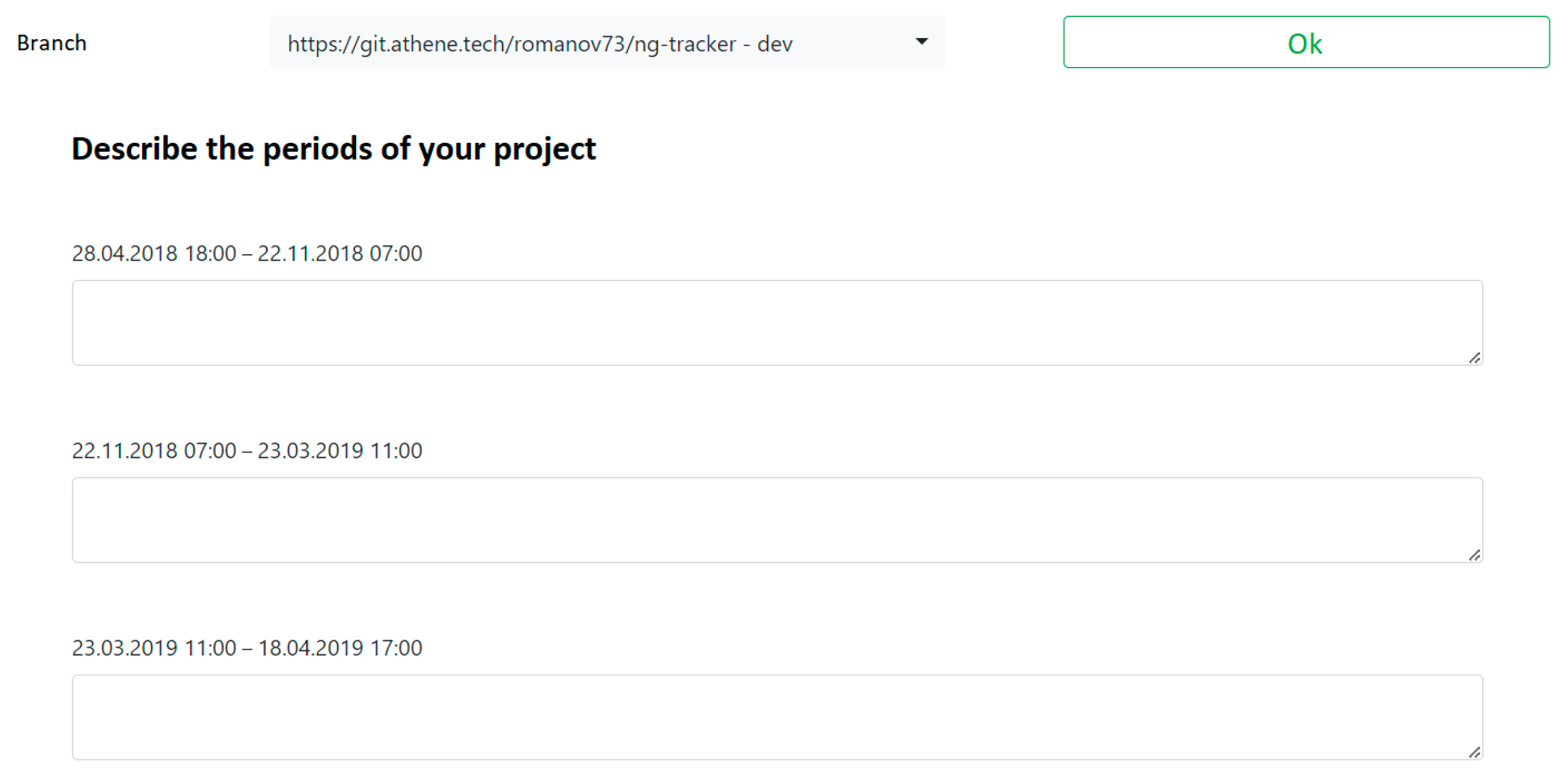
  • 28 April 2018–22 November 2018: Project start phase. Students include libraries in the project and create the basis for further development;
  • 22 November 2018–23 March 2019: Collective development start phase. There was an active change in the project but students duplicate some code due to lack of knowledge of the project features;
  • 23 March 2019–18 April 2019: Active development phase. Students were required to implement all functional requirements and present a demo of their part of the work;
  • 18 April 2019–2 November 2020: Phase of correcting defects, removing duplicate code and optimization.
Figure 2 shows these time intervals superimposed on the time series.
It is necessary to interview an expert to describe the state of the project in the allocated time intervals under step 5 of the model training algorithm. The expert is asked to fill out the form to describe the project condition in these selected time intervals, see Figure 3.
The time intervals characteristic allows us to establish the fuzzy rules. The approach forms the following rules in according to equation 1 for a project that was known to the expert (https://git.athene.tech/romanov73/ng-tracker (accessed on 26 October 2023)), see Table 4.
The proposed approach result is the consequence of the activated rules based on the predicted tendencies of the time series (in accordance with the evaluation algorithm). For example, as shown in Figure 4, there may be several conclusions for a project.
This project was analyzed on time series that fulfill the same rules to evaluate the adequacy of the offered rule generation method. The system has achieved a 100% match with the expert inferences during the markup phase.
Evaluation of the source code repositories can be measured in both the expert workload during data markup and in the time it took to analyze the current repository.
Firstly, we need to evaluate the expert workload. This evaluation needs to be based on the number of time intervals selected in the project, since they will need to be characterized by the expert. For the entire source data set, the following results were reached. These results reflect both the amount of time it took to select the intervals and the number of selected intervals, see Table 5.
Figure 5 visualizes the relationship between time cost for analysis and the size of the repository.
This figure shows that the time it takes to select the time intervals strongly depends on the repository size. It should also be noted that this time also depends on the commit size, i.e., the number of lines affected by the commit.
The second part of the experiment performs an analysis of the time it takes to analyze the repository to evaluate it using the features of the IT project hosting services and the software system that implements the evaluation method. The measurement will consist of determining the time taken by the expert during the evaluation process. The following actions were proposed to be included:
  • Determining the complexity of the project based on its commit history. This action is required at the start of the analysis to select a project with a similar history;
  • Determining the project condition based on its development stage. The number of opened/closed tasks, the number of developers and the number of developers making commits are determined;
  • Determining the structural complexity of the project based on its file analysis (such as number of classes, their types, etc.);
  • Determining the actuality of the project based on code change history, task activity and the number of marks the repository received from other users.
The repositories from the source data set are analyzed and the time it took for the operator to complete the task is measured based on the operation list, see Table 6. The repositories are listed in Table 3. The page to load time for every repository selected was 5 s.
On average, the time it took to complete the analysis shrank by a factor of 4. However, for some tasks, the hosting services still hold an advantage. Another flaw is the requirement to select the time intervals beforehand. This action is not required often and is only needed during the learning process.

6. Conclusions

The completed experiments showed the effectiveness of the suggested forecast method; the time cost for repository analysis was shortened by a factor of 4 on average. Various repository evaluation methods were described and researched. A method that allows the repository evaluation based on analyzing the dynamic of its metrics was developed.
The following actions were performed:
-
Numeric metrics for the source code repositories and IT project hosting services, that are used for analyzing the change dynamic, were determined;
-
The algorithms for selecting and extracting time series were developed;
-
An algorithm for forming a fuzzy rule base based on marked data was developed;
-
An algorithm for evaluating the software repositories was developed.
The limitations of this approach are as follows:
  • Time series might not have enough length to calculate the trends and create a forecast, or some of the time series might not be able to be built for repositories with a short history. This leads to an impossibility for the repository analysis;
  • The rules will not reflect the actual values for time series trends if an expert has created a rule base for a project that does not match the trends of the current project;
  • There is a large amount of workload for the expert, and prohibitive time costs for large projects with a long history. The analysis time is based on analyzing the source code of every commit in the project history. This also leads to the time series becoming increasingly large in length, forcing the expert to evaluate each time interval separately.
The development of this approach will be integrated with the previously presented approach to contextually analyze the dynamics of the control system indicators [25]. We provided a comparison of the manual analysis and proposed an approach in terms of time spent on analysis operations. An evaluation of increasing the efficiency of the project management from the point of view of the decision maker is also needed in future work.

Author Contributions

Conceptualization, N.Y. and S.K.; Software, P.S. and I.A.; Formal analysis, A.R. and A.F. All authors have read and agreed to the published version of the manuscript.

Funding

This study was supported the Ministry of Science and Higher Education of Russia in framework of project No. 075-03-2023-143 «The study of intelligent predictive analytics based on the integration of methods for constructing features of heterogeneous dynamic data for machine learning and methods of predictive multimodal data analysis».

Data Availability Statement

Data are contained within the article.

Conflicts of Interest

The authors declare no conflicts of interest.

References

  1. GitHub. Available online: https://github.com (accessed on 26 October 2023).
  2. GitLab. Available online: https://gitlab.com (accessed on 26 October 2023).
  3. Bitbucket. Available online: https://bitbucket.org (accessed on 26 October 2023).
  4. Rating of Repository Services for Storing Code. Available online: https://tagline.ru/source-code-repository-rating/2016 (accessed on 26 October 2023).
  5. GitHub Repository to Learn Data Science. Available online: https://levelup.gitconnected.com/top-10-github-repository-to-learn-data-science-892935bcebdb (accessed on 26 October 2023).
  6. Repository for Research Work at Bauman MSTU. Available online: https://github.com/iu5git/Science (accessed on 26 October 2023).
  7. Neural-Style. Available online: https://github.com/jcjohnson/neural-style (accessed on 26 October 2023).
  8. Git. Available online: https://git-scm.com (accessed on 26 October 2023).
  9. Mercurial. Available online: https://www.mercurial-scm.org (accessed on 26 October 2023).
  10. Subversion. Available online: https://subversion.apache.org (accessed on 26 October 2023).
  11. CVS. Available online: https://cvs.nongnu.org (accessed on 26 October 2023).
  12. Filippov, A.; Romanov, A.; Skalkin, A.; Stroeva, J.; Yarushkina, N. Approach to Formalizing Software Projects for Solving Design Automation and Project Management Tasks. Software 2023, 2, 133–162. [Google Scholar] [CrossRef]
  13. Muna, A. Assessing programming language impact on software development productivity based on mining oss repositories. ACM SIGSOFT Softw. Eng. Notes 2022, 44, 36–38. [Google Scholar] [CrossRef]
  14. Abuhamad, M.; Rhim, J.S.; AbuHmed, T.; Ullah, S.; Kang, S.; Nyang, D. Code authorship identification using convolutional neural networks. Future Gener. Comput. Syst. 2019, 95, 104–115. [Google Scholar] [CrossRef]
  15. Zhang, Y.; Wang, T. CCEyes: An Effective Tool for Code Clone Detec-tion on Large-Scale Open Source Repositories. In Proceedings of the 2021 IEEE International Conference on Information Communication and Software Engineering (ICICSE), Chengdu, China, 19–21 March 2021; pp. 61–70. [Google Scholar]
  16. Heinze, T.S.; Stefanko, V.; Amme, W. Mining BPMN Processes on GitHub for tool validation and development. In Enterprise, Business-Process and Information Systems Modeling: 21st International Conference, BPMDS 2020, 25th International Conference, EMMSAD 2020, Held at CAiSE 2020, Grenoble, France, 8–9 June 2020; Springer International Publishing: Berlin/Heidelberg, Germany, 2020; Proceedings 21; pp. 193–208. [Google Scholar]
  17. Le, T.H.M.; Chen, H.; Babar, M.A. Deep learning for source code modeling and generation: Models, applications, and challenges. ACM Comput. Surv. (CSUR) 2020, 53, 1–38. [Google Scholar] [CrossRef]
  18. Thota, M.K.; Shajin, F.H.; Rajesh, P. Survey on software defect prediction techniques. Int. J. Appl. Sci. Eng. 2020, 17, 331–344. [Google Scholar]
  19. Arndt, N.; Martin, M. Decentralized collaborative knowledge management using git. In Proceedings of the Companion Proceedings of The 2019 World Wide Web Conference, San Francisco, CA, USA, 13–17 May 2019; pp. 952–953. [Google Scholar]
  20. Scrum. Available online: https://www.scrum.org/learning-series/what-is-scrum (accessed on 26 October 2023).
  21. Manifest Agile. Available online: http://agilemanifesto.org/iso/ru/manifesto.html (accessed on 26 October 2023).
  22. Ge, P.; Wang, J.; Ren, P.; Gao, H.; Luo, Y. A new improved forecasting method integrated fuzzy time series with exponential smoothing method. Int. J. Environ. Pollut. 2013, 51, 206–221. [Google Scholar] [CrossRef]
  23. Viertl, R. Statistical Methods for Fuzzy Data; John Wiley & Sons, Ltd.: Hoboken, NJ, USA, 2011; 270p. [Google Scholar]
  24. CIF Dataset. Available online: https://irafm.osu.cz/cif2015/main.php (accessed on 26 October 2023).
  25. Romanov, A.A.; Filippov, A.A.; Voronina, V.V.; Guskov, G.; Yarushkina, N.G. Modeling the Context of the Problem Domain of Time Series with Type-2 Fuzzy Sets. Mathematics 2021, 9, 2947. [Google Scholar] [CrossRef]
Figure 1. Time series of project commits (date format is dd.mm.yyyy).
Mathematics 12 00047 g001
Figure 2. Time series of project commits with highlighted time intervals (date format is dd.mm.yyyy).
Mathematics 12 00047 g002
Figure 3. Expert description fill-out form (date format is dd.mm.yyyy).
Mathematics 12 00047 g003
Figure 4. Example of project conclusions.
Mathematics 12 00047 g004
Figure 5. Relationship between time needed to select the intervals and the size of the repository.
Mathematics 12 00047 g005
Table 1. Models used in the research.
ARIMAAutoARIMAStatsForecastAutoARIMA
ExponentialSmoothingStatsForecastAutoCESTheta
FourThetaStatsForecastAutoThetaFFT
KalmanForecasterCrostonRandomForest
RegressionModelLinearRegressionModelLightGBMModel
CatBoostModelXGBModelRNNModel
BlockRNNModelNBEATSModelNHiTSModel
TCNModelTransformerModelTFTModel
DLinearModelNLinearModel-
Table 2. Forecast method ranking based on quality.
MethodNumber of Predicted Time
Series
FFT27
MultTrendMultSeasonality12
MultTrendAddSeasonality10
AddTrendMultSeasonality5
RNNModel (LSTM)5
RNNModel (Vanilla RNN)3
NBEATSModel2
TransformerModel2
ARIMA1
CatBoostModel1
DATrendAddSeasonality1
DATrendMultSeasonality1
DLinearModel1
Fuzzy (Add,Add)1
FuzzyWithSets (Add,Add)1
FuzzyWithSets (Add,Mult)1
LightGBMModel1
NoTrendMultSeasonality1
TFTModel1
Table 3. Software repositories.
Repository LinkRepository Characteristic
https://github.com/killjoy1221/TabbyChat-2
(accessed on 26 October 2023)
An open repository with many developers and small number of commits. Used for testing models.
https://github.com/helix-editor/helix
(accessed on 26 October 2023)
An open repository with many developers. Used for testing models.
https://github.com/apache/commons-lang
(accessed on 26 October 2023)
An open repository with many developers and large number of commits. Used for testing models.
https://git.athene.tech/romanov73/spring-mvc-example (accessed on 26 October 2023)A repository with a small number of commits, one developer and a known development process. Used for testing models.
https://git.athene.tech/romanov73/ng-tracker
(accessed on 26 October 2023)
A repository with a known development process. Used for training models.
https://git.athene.tech/romanov73/git-extractor
(accessed on 26 October 2023)
A repository with a known development process. Used for testing models.
Table 4. Extracted rules.
CriteriaTrend CriteriaTrend Inference
IfTask time seriesgrowandBranch time seriesgrowthenSome level of activity, likely starting a project
IfTask time seriesgrowandStar time seriesgrowthenSome level of activity, likely starting a project
IfBranch time seriesgrowandStar time seriesgrowthenSome level of activity, likely starting a project
IfBranch time seriesshrinkandStar time seriesshrinkthenPeriod of quick fixes
IfEntity time seriesgrowandCommit time seriesgrowthenTesting technology, creating the MVP of an app.
IfEntity time seriesshrinkandCommit time seriesshrinkthenUser education
IfEntity time seriesgrowandCommit time seriesgrowthenActive work of several users
IfEntity time seriesshrinkandCommit time seriesshrinkthenActive task completion
IfBranch time seriesstableandStar time seriesstablethenSmall fixes
IfBranch time seriesstableandTask time seriesstablethenSmall fixes
IfStar time seriesstableandTask time seriesstablethenSmall fixes
Table 5. Number of time intervals in analyzed projects.
Repository LinkNumber of CommitsTime for Selecting the Time IntervalsNumber of Selected Time Intervals
https://github.com/killjoy1221/TabbyChat-2
(accessed on 26 October 2023)
3231202
https://github.com/helix-editor/helix
(accessed on 26 October 2023)
464819632
https://github.com/apache/commons-lang
(accessed on 26 October 2023)
718440205
https://git.athene.tech/romanov73/spring-mvc-example (accessed on 26 October 2023)3102
https://git.athene.tech/romanov73/ng-tracker
(accessed on 26 October 2023)
920204
https://git.athene.tech/romanov73/git-extractor
(accessed on 26 October 2023)
298607
Table 6. Repository analysis time costs.
Repository LinkNumber of the Operation
(Manual/Suggested Way), Seconds
1234
https://github.com/killjoy1221/TabbyChat-2
(accessed on 26 October 2023)
5/1010/1425/1420/14
https://github.com/helix-editor/helix
(accessed on 26 October 2023)
5/10175/15310/1520/15
https://github.com/apache/commons-lang
(accessed on 26 October 2023)
5/10125/15478/1520/15
https://git.athene.tech/romanov73/spring-mvc-example
(accessed on 26 October 2023)
5/105/125/1220/12
https://git.athene.tech/romanov73/ng-tracker
(accessed on 26 October 2023)
5/1045/1655/1620/16
https://git.athene.tech/romanov73/git-extractor
(accessed on 26 October 2023)
5/1025/1620/1620/16
Total564.1148.820
/////
Average1014.614.614.6
Disclaimer/Publisher’s Note: The statements, opinions and data contained in all publications are solely those of the individual author(s) and contributor(s) and not of MDPI and/or the editor(s). MDPI and/or the editor(s) disclaim responsibility for any injury to people or property resulting from any ideas, methods, instructions or products referred to in the content.

