Some Inverse Problems of Two-Dimensional Stokes Flows by the Method of Fundamental Solutions and Kalman Filter

Abstract

Some inverse problems of Stokes flow, including noisy boundary conditions, unknown angular velocity, and dynamic viscous constant identification are studied in this paper. The interpolation equations for those inverse problems are constructed using the method of fundamental solutions (MFS). Based on the noise addition technique, the inverse problems are solved using MFS and a Kalman filter. It is seen from numerical experiments that these approaches and algorithms are valid and have strong robustness and high accuracy in solving inverse Stokes problems.

1. Introduction

Stokes flows are utilized in many interdisciplinary fields [1], and they have attracted more and more studies for the properties of the velocity and pressure fields. For steady Stokes flows, the stream and pressure functions of the Stokes flows are in simple forms of bi-harmonic and harmonic style, which can be found in the next section. Thus, the solutions of those bi-harmonic and harmonic equations have usually been addressed by classical numerical methods, e.g., the finite element method (FEM), the finite difference method (FDM) [2], the radial basis functions method (RBF) [3,4], the Galerkin method [5,6,7], the method of fundamental solutions (MFS) [8,9,10,11,12] or other boundary collocation method [13], etc. The MFS was selected or use in the computation of Stokes problems, because it is a simple concept, a true boundary meshfree method, and is easy to implement. It has the flexibility of using various forms of fundamental solutions, singular, nonsingular, and mixing with general solutions and particular solutions, for different purposes [12]. Although the MFS’s interpolation matrix is ill-conditioned, regularization methods can help to find the optimal stable MFS scheme [14]. Based on the MFS with Stokeslets, Young et al. [15] solved the Stokes problem of lid-driven flows in the square cavity, cubic cavity, and wave-shaped bottom domain. They concluded that the MFS was more computationally efficient than the FEM in dealing with an irregularly shaped domain. Stokes flow problems set in a rectangular cavity including circular cylinders have been studied by Young et al. [16] with the help of MFS utilizing Stokeslets. It is found in their paper that the MFS is efficient and simple to implement as compared to the mesh-dependent schemes. For the other forms of fundamental solutions utilized in the MFS, Alves and Silvestre [17] established new density results based on the trace spaces in terms of Stokeslets. Derived density equations were applied to solve the boundary value problems of Stokes equations. Young et al. [18] developed a pressure-stream function formulation to solve two-dimensional and three-dimensional Stokes flows using the MFS with classic fundamental solutions, which were different from those using Stokeslets. In their paper, the fields of pressure, velocity, vorticity, stream function, and traction forces could be solved simultaneously.

A great many of the studies, such as those mentioned above, discussed the direct problems of the Stokes flow. The inverse problem of Stokes flow is another important topic to be studied, since it must be solved to determine an optimal design in engineering. Since data describing the direct problem are not available, a direct numerical solver should be called repeatedly in an iterative process to obtain or reconstruct the real state. Karageorghis et al. [19,20] solved the inverse problem with respect to Brinkman fluid flows, including obstacles of unknown shapes for the exterior and interior problems. In their papers, they also proved the stability and accuracy of their proposed numerical technique by numerical examples. Using the modified collocation Trefftz method, Fan and Li [21] studied an inverse Stokes problem involving unknown boundary conditions. Their numerical examples showed that their proposed scheme offered good accuracy and stability. Fan et al. [22] proposed a theoretical method to determine the viscous coefficient in the Navier-Stokes equation by analyzing observation data in a neighborhood of the boundary. In their paper, Lipschitz stability was proved by Carleman estimates in Sobolev spaces, though they did not give a numerical example to show its effectiveness.

Motivated by the rapidly growing interest in inverse Stokes problems, we applied MFS and the Kalman filter technique to some inverse problems, including field value reconstruction and velocity and dynamic viscous constant identifications. Karageorghis et al. [23] noted that the MFS is an ideal candidate for efficiently solving inverse problems in complicated geometries and in higher dimensions, since it has the advantages of easy implementation, fast computation, lower storage requirements, and exponential convergence. The Kalman filter includes a set of mathematical equations that provide an efficient recursive means to estimate the real state, in a way that minimizes the mean of the squared errors [24]. The filter is therefore one of the most powerful tools applicable to this kind of problem. It supports estimations even when the precise nature of the modeled system is unknown [25]. Villenas and Vargas et al. [26] considered a homogeneous platoon with vehicles that communicate through channels prone to data loss, based on the Kalman compensation strategy. In their paper, it was shown that their proposed method could achieve relative stability under the mean and variance of tracking and estimation errors. Zhang et al. [27] presented a method for online calibration of pitot tubes and wind field estimation with the help of an extended Kalman filter. Their numerical simulations and flight experiment results agree with each other, validating the proposed method. Using the Kalman filter, Dogariu et al. [28] addressed the identification of linearly separable systems with the help of decomposition techniques. Their simulation results showed that the proposed Kalman filter offered good performance for multi-linear forms. Tamuly et al. [29] proposed a method to identify damage in a reinforced concrete structure with the help of a Kalman filter. In their simulation, the adaptation of the material parameter estimation and experimental data agreed well. Kalman filters are also utilized in groundwater pollution source identification [30], charge estimation for lithium-ion batteries [31], protection strategies for microgrids [32], and neural networks [33], etc.

As mentioned before, Stokes flows can be utilized in many interdisciplinary fields. Most researchers have focused on the direct problems of the velocity and pressure fields. For these direct problems, one can determine the solutions of the boundary and initial conditions governed by the control equations of Stokes flow in a relatively simple manner. In contrast, the inverse problems of Stokes flows are more difficult to solve than direct ones because they are ill-posed. Furthermore, in order to solve an inverse problem, a direct solver (e.g., FEM, FDM and RBF, etc.) must be called repeatedly as part of a complex iterative procedure. In particular, small errors in the measured data may lead to large errors in the solution. These errors make inverse problems of Stokes flows difficult to solve. In this paper, the MFS and Kalman filter are first employed to solve the inverse problems, including the field value reconstruction and velocity and dynamic viscous constant identifications for Stokes flow. In practice, the boundary conditions of Stokes problems inevitably involve noise. An approach to field value reconstruction based on the Kalman filter is given in this paper. Furthermore, schemes are developed to identify the angular velocity and dynamic viscous constant. In those identifications, the angular velocity and dynamic viscous constant are treated as unknowns that can be solved simultaneously with the coefficients in the interpolation equations (interpolation equations). It is noted that the interpolation matrices of these inverse problems are more severely ill-conditioned than those of direct problems. It is known that the ill-condition is induced by the overfitting of the boundary conditions on the boundary nodes. One of the possible remedies for the overfitting is a noise addition technique [34,35,36]. Therefore, we propose an approach to obtain the optimal objective value (angular velocity or viscous constant) by using a Kalman filter after injecting Gaussian white noises into the boundary conditions. The algorithms for those inverse problems are also given. Furthermore, an approach to the exterior problem of a Stokes flow, which is different from an inverse problem according to Ref. [19], is also presented in this paper. The interpolation equations for an exterior (unbounded) problem of Stokes flow have been developed by considering uniform boundary conditions at infinite. The numerical examples show that the presented method has strong robustness even if there is noise.

A brief outline of this paper is as follows. In Section 2, the governing equations and fundamental solutions (Stokeslets) are presented. In Section 3, the formulations of the MFS and the Kalman filter are given. It is noted here that the MFS formulations for direct exterior problems are also derived in Section 3. In Section 4, the inverse problems are addressed in detail. The basic equations and algorithms for those inverse problems are presented. In Section 5, four numerical experiments are performed to verify the effectiveness of the proposed approaches to the inverse problems. Some conclusions are drawn in the last section.

2. Governing Equations and Fundamental Solutions

According to Newtonian viscous law, the constitutive equation for the Stokes flow can be represented as

$${\sigma }_{ij}=2\mu {\epsilon }_{ij}-p{\delta }_{ij}$$

(1)

where ${\sigma }_{ij}$ is the stress component, $\mu$ is the dynamic viscous constant, $p$ is the pressure, ${\delta }_{ij}$ is Kronecker Delta, and $D_{ij}$ is the strain rate component, which can be given by

$$D_{ij}=\frac{1}{2}(\frac{\partial u_i}{\partial x_j}+\frac{\partial u_j}{\partial x_i})$$

(2)

where $u_i$ ($i=1,2$) represents the axis component of vector $\mathit{x}=(x_1,x_2)$ in a Cartesian coordinate system, and $u_i$ ($i=1,2$) is the component of velocity vector $\mathit{u}=(u_1,u_2)$.

If the body (mass) force is neglected and the Reynolds number is small, the momentum equation of a stationary Stokes flow can be given as follows:

$$\frac{\partial {\sigma }_{ij}}{\partial x_j}=0$$

(3)

where the Einstein summation convention is applied for the repeated index. The repeated indices in the following equations adopt the Einstein summation convention, if they are not otherwise specified.

Additionally, the continuity equation is given as

$$\frac{\partial u_i}{\partial x_i}=0$$

(4)

for incompressible flow.

Substituting Equations (1) and (2) into Equation (3), we have

$$-\frac{\partial p}{\partial x_i}+\mu \left(\frac{{\partial }^2}{\partial x_1^2}+\frac{{\partial }^2}{\partial x_2^2}\right)u_i=0$$

(5)

where $i=1,2$ for two-dimensional Stokes problems.

In practice, Equations (3) and (5) are the governing equations for Stokes problems in domain $\mathsf{\Omega }$ with the corresponding boundary conditions:

$$u_i={\overline{u}}_i \mathrm{on} \partial {\mathsf{\Omega }}_u,$$

(6)

and

$${\sigma }_{ij}{n}_j={\overline{t}}_i \mathrm{on} \partial {\mathsf{\Omega }}_t,$$

(7)

where ${\overline{u}}_i$ and ${\overline{t}}_i$ are the known velocity and traction on the boundaries $\partial {\mathsf{\Omega }}_u$ and $\partial {\mathsf{\Omega }}_t$ ($\partial {\mathsf{\Omega }}_u+\partial {\mathsf{\Omega }}_t=\partial {\mathsf{\Omega }}_t$), respectively. $n_j$ is the normal component on boundary $\partial {\mathsf{\Omega }}_t$.

According to the continuity Equation (4), we have

$${\displaystyle \underset{\mathsf{\Omega }}{\iint }\frac{\partial u_i}{\partial x_i}\mathrm{d}\mathit{A}}={\displaystyle \underset{\partial \mathsf{\Omega }}{\oint }{u}_i{n}_i\mathrm{d}s}={\displaystyle \underset{\partial \mathsf{\Omega }}{\oint }(u_1\mathrm{d}{x}_2+u_2\mathrm{d}{x}_1)}=0$$

(8)

where the relations $n_1=\mathrm{d}{x}_2/\mathrm{d}s$ and $n_2=-\mathrm{d}{x}_1/\mathrm{d}s$ are used.

Thus, there exists a function $\mathsf{\Psi }$ expressed by

$$\mathrm{d}\mathsf{\Psi }=\frac{\partial \mathsf{\Psi }}{\partial x_i}\mathrm{d}{x}_i$$

(9)

which satisfies

$$u_1=\frac{\partial \mathsf{\Psi }}{\partial x_2}, u_2=-\frac{\partial \mathsf{\Psi }}{\partial x_1},$$

(10)

where $\mathsf{\Psi }$ is called the stream function.

With help of Equations (3) and (10), we have

$${\left(\frac{{\partial }^2}{\partial x_1^2}+\frac{{\partial }^2}{\partial x_2^2}\right)}^2\mathsf{\Psi }=0, \left(\frac{{\partial }^2}{\partial x_1^2}+\frac{{\partial }^2}{\partial x_2^2}\right)p=0.$$

(11)

From Equation (11), one can see that the stream function $\mathsf{\Psi }$ and pressure $p$ satisfy the biharmonic equation and the Laplace equation, respectively. The fundamental solutions for a Stokes flow can be derived by applying concentrated point forces $f_i$ ($i=1,2$) at location ${\mathit{x}}^{\prime }=({x_1}^{\prime },{x_2}^{\prime })$ as follows:

$$-\frac{\partial p}{\partial x_i}+\mu \left(\frac{{\partial }^2}{\partial x_1^2}+\frac{{\partial }^2}{\partial x_2^2}\right)u_i=-f_i\delta (‖\mathit{x}-{\mathit{x}}^{\prime }‖)$$

(12)

where $‖\mathit{x}-{\mathit{x}}^{\prime }‖$ represents the Euclidean distance between $\mathit{x}$ and ${\mathit{x}}^{\prime }$.

By considering Equations (4) and (10), the two-dimensional fundamental solutions of the velocity and pressure can be obtained as [16]

$$\begin{array}{l}{u}_1^{*}(\mathit{x},{\mathit{x}}^{\prime })=\frac{1}{8\pi \mu }\left\{f_1\left[-2\ln ||\mathit{x}-{\mathit{x}}^{\prime }||+\frac{2{(x_1-x_1^{\prime })}^2}{||\mathit{x}-{\mathit{x}}^{\prime }|{|}^2}-3\right]\right.\\ \hspace{0.17em}\hspace{0.17em}\hspace{0.17em}\hspace{0.17em}\hspace{0.17em}\hspace{0.17em}\hspace{0.17em}\hspace{0.17em}\hspace{0.17em}\hspace{0.17em}\left.+f_2\left[\frac{2(x_1-x_1^{\prime })(x_2-x_2^{\prime })}{||\mathit{x}-{\mathit{x}}^{\prime }|{|}^2}\right]\right\},\end{array}$$

(13)

$$\begin{array}{l}{u}_2^{*}(\mathit{x},{\mathit{x}}^{\prime })=\frac{1}{8\pi \mu }\left\{f_1\left[\frac{2(x_1-x_1^{\prime })(x_2-x_2^{\prime })}{||\mathit{x}-{\mathit{x}}^{\prime }|{|}^2}\right]\right.\\ \hspace{0.17em}\hspace{0.17em}\hspace{0.17em}\hspace{0.17em}\hspace{0.17em}\hspace{0.17em}\hspace{0.17em}\hspace{0.17em}\hspace{0.17em}\left.+f_2\left[-2\ln ||\mathit{x}-{\mathit{x}}^{\prime }||+\frac{2{(x_2-x_2^{\prime })}^2}{||\mathit{x}-{\mathit{x}}^{\prime }|{|}^2}-3\right]\right\},\end{array}$$

(14)

$$p^{*}(\mathit{x},{\mathit{x}}^{\prime })=\frac{1}{2\pi }\left(f_1\frac{x_1-x_1^{\prime }}{||\mathit{x}-{\mathit{x}}^{\prime }|{|}^2}+f_2\frac{x_2-x_2^{\prime }}{||\mathit{x}-{\mathit{x}}^{\prime }|{|}^2}\right),$$

(15)

$$\begin{array}{l}{\mathsf{\Psi }}^{*}(\mathit{x},{\mathit{x}}^{\prime })=\frac{1}{8\pi \mu }\left\{f_1\left[-(x_2-x_2^{\prime })(2\ln ||\mathit{x}-x\mathit{\prime }||+1)\right]\right.\\ \hspace{0.17em}\hspace{0.17em}\hspace{0.17em}\hspace{0.17em}\hspace{0.17em}\hspace{0.17em}\hspace{0.17em}\hspace{0.17em}\hspace{0.17em}\left.+f_2\left[(x_1-x_1^{\prime })(2\ln ||\mathit{x}-{\mathit{x}}^{\prime }||+1)\right]\right\},\end{array}$$

(16)

where $u_1^{*}(\mathit{x},{\mathit{x}}^{\prime })$, $u_2^{*}(\mathit{x},{\mathit{x}}^{\prime })$, $p^{*}(\mathit{x},{\mathit{x}}^{\prime })$ and ${\mathsf{\Psi }}^{*}(\mathit{x},{\mathit{x}}^{\prime })$ are called Stokeslets.

One can make Equations (5) and (12) dimensionless by using viscous scales as reference scales. When a length-scale l determined by domain size is used, the reference velocity u_i = μ/(ρl) (i = 1, 2) can be applied to make Equations (5) and (12) dimensionless. Thus, Equations (5), (12)–(16) have a unit coefficient μ = 1 for the viscous term.

Furthermore, the so-called stresslets ${\sigma }_{ij}^{*}(\mathit{x},{\mathit{x}}^{\prime })$ can also be given as:

$${\sigma }_{11}^{*}(\mathit{x},{\mathit{x}}^{\prime })=-\frac{1}{\pi }\left\{f_1\left[\frac{{(x_1-x_1^{\prime })}^3}{||\mathit{x}-{\mathit{x}}^{\prime }|{|}^4}\right]+f_2\left[\frac{{(x_1-x_1^{\prime })}^2(x_2-x_2^{\prime })}{||\mathit{x}-{\mathit{x}}^{\prime }|{|}^4}\right]\right\}$$

(17)

$${\sigma }_{22}^{*}(\mathit{x},{\mathit{x}}^{\prime })=-\frac{1}{\pi }\left\{f_1\left[\frac{{(x_2-x_2^{\prime })}^3}{||\mathit{x}-{\mathit{x}}^{\prime }|{|}^4}\right]+f_2\left[\frac{{(x_2-x_2^{\prime })}^2(x_1-x_1^{\prime })}{||\mathit{x}-{\mathit{x}}^{\prime }|{|}^4}\right]\right\}$$

(18)

$${\sigma }_{12}^{*}(\mathit{x},{\mathit{x}}^{\prime })={\sigma }_{21}^{*}(\mathit{x},{\mathit{x}}^{\prime })=-\frac{1}{\pi }\left\{f_1\left[\frac{{(x_1-x_1^{\prime })}^2(x_2-x_2^{\prime })}{||\mathit{x}-{\mathit{x}}^{\prime }|{|}^4}\right]+f_2\left[\frac{{(x_2-x_2^{\prime })}^2(x_1-x_1^{\prime })}{||\mathit{x}-{\mathit{x}}^{\prime }|{|}^4}\right]\right\}.$$

(19)

The Stokeslets and stresslets can be utilized as basis functions for MFS, which will be discussed in the following section.

3. MFS and Kalman Filter Formulas

3.1. MFS Formulas

3.1.1. Formulas for Bounded Domains

According to the concepts of MFS, the approximate solutions $\mathsf{\Psi }(\mathit{x})$, $u_i(\mathit{x})$, $p(\mathit{x})$ and ${\sigma }_{ij}(\mathit{x})$ of the stream, velocity, pressure, and stress fields can be calculated:

$$\begin{array}{l}\mathsf{\Psi }(\mathit{x})=\frac{1}{8\pi \mu }\left\{{\displaystyle \sum _{j=1}^N{\alpha }_j\left[-(x_2-x_{2j}^{\prime })(2\ln ||\mathit{x}-\mathit{x}{\prime }_j||+1)\right]}\right.\\ \hspace{0.17em}\hspace{0.17em}\hspace{0.17em}\hspace{0.17em}\hspace{0.17em}\hspace{0.17em}\hspace{0.17em}\hspace{0.17em}\hspace{0.17em}\hspace{0.17em}\hspace{0.17em}\hspace{0.17em}\hspace{0.17em}\left.+{\displaystyle \sum _{j=1}^N{\beta }_j\left[(x_1-x_{1j}^{\prime })(2\ln ||\mathit{x}-\mathit{x}{\prime }_j||+1)\right]}\right\},\end{array}$$

(20)

$$\begin{array}{l}{u}_1(\mathit{x})=\frac{1}{8\pi \mu }\left\{{\displaystyle \sum _{j=1}^N{\alpha }_j\left[-2\ln ||\mathit{x}-\mathit{x}{\prime }_j||+\frac{2{(x_1-x_{1j}^{\prime })}^2}{||\mathit{x}-\mathit{x}{\prime }_j|{|}^2}-3\right]}\right.\\ \hspace{0.17em}\hspace{0.17em}\hspace{0.17em}\hspace{0.17em}\hspace{0.17em}\hspace{0.17em}\hspace{0.17em}\hspace{0.17em}\hspace{0.17em}\hspace{0.17em}\hspace{0.17em}\hspace{0.17em}\left.+{\displaystyle \sum _{j=1}^N{\beta }_j\left[\frac{2(x_1-x_{1j}^{\prime })(x_2-x_{2j}^{\prime })}{||\mathit{x}-\mathit{x}{\prime }_j|{|}^2}\right]}\right\},\end{array}$$

(21)

$$\begin{array}{l}{u}_2(\mathit{x})=\frac{1}{8\pi \mu }\left\{{\displaystyle \sum _{j=1}^N{\alpha }_j\left[\frac{2(x_1-x_{1j}^{\prime })(x_2-x_{2j}^{\prime })}{||\mathit{x}-\mathit{x}{\prime }_j|{|}^2}\right]}\right.\\ \hspace{0.17em}\hspace{0.17em}\hspace{0.17em}\hspace{0.17em}\hspace{0.17em}\hspace{0.17em}\hspace{0.17em}\hspace{0.17em}\hspace{0.17em}\hspace{0.17em}\hspace{0.17em}\hspace{0.17em}\hspace{0.17em}\left.+{\displaystyle \sum _{j=1}^N{\beta }_j\left[-2\ln ||\mathit{x}-\mathit{x}{\prime }_j||+\frac{2{(x_2-x_{2j}^{\prime })}^2}{||\mathit{x}-\mathit{x}{\prime }_j|{|}^2}-3\right]}\right\},\end{array}$$

(22)

$$p(\mathit{x})=\frac{1}{2\pi }\left({\displaystyle \sum _{j=1}^N{\alpha }_j\frac{x_1-x_{1j}^{\prime }}{||\mathit{x}-\mathit{x}{\prime }_j|{|}^2}}+{\displaystyle \sum _{j=1}^N{\beta }_j\frac{x_2-x_{2j}^{\prime }}{||\mathit{x}-\mathit{x}{\prime }_j|{|}^2}}\right)$$

(23)

$${\sigma }_{11}^{*}(\mathit{x})=-\frac{1}{\pi }\left\{{\displaystyle \sum _{j=1}^N{\alpha }_j\left[\frac{{(x_1-x_{1j}^{\prime })}^3}{||\mathit{x}-\mathit{x}{\prime }_j|{|}^4}\right]}+{\displaystyle \sum _{j=1}^N{\beta }_j\left[\frac{{(x_1-x_{1j}^{\prime })}^2(x_2-x_{2j}^{\prime })}{||\mathit{x}-\mathit{x}{\prime }_j|{|}^4}\right]}\right\}$$

(24)

$${\sigma }_{22}^{*}(\mathit{x})=-\frac{1}{\pi }\left\{{\displaystyle \sum _{j=1}^N{\alpha }_j\left[\frac{{(x_2-x_{2j}^{\prime })}^3}{||\mathit{x}-\mathit{x}{\prime }_j|{|}^4}\right]}+{\displaystyle \sum _{j=1}^N{\beta }_j\left[\frac{{(x_2-x_{2j}^{\prime })}^2(x_1-x_{1j}^{\prime })}{||\mathit{x}-\mathit{x}{\prime }_j|{|}^4}\right]}\right\}$$

(25)

$$\begin{array}{l}{\sigma }_{12}^{*}(\mathit{x})={\sigma }_{21}^{*}(\mathit{x})=-\frac{1}{\pi }\left\{{\displaystyle \sum _{j=1}^N{\alpha }_j\left[\frac{{(x_1-x_{1j}^{\prime })}^2(x_2-x_{2j}^{\prime })}{||\mathit{x}-\mathit{x}{\prime }_j|{|}^4}\right]}\right.\\ \hspace{0.17em}\hspace{0.17em}\hspace{0.17em}\hspace{0.17em}\hspace{0.17em}\hspace{0.17em}\hspace{0.17em}\hspace{0.17em}\hspace{0.17em}\hspace{0.17em}\hspace{0.17em}\hspace{0.17em}\hspace{0.17em}\hspace{0.17em}\hspace{0.17em}\hspace{0.17em}\hspace{0.17em}+\left.{\displaystyle \sum _{j=1}^N{\beta }_j\left[\frac{{(x_2-x_{2j}^{\prime })}^2(x_1-x_{1j}^{\prime })}{||\mathit{x}-\mathit{x}{\prime }_j|{|}^4}\right]}\right\},\end{array}$$

(26)

where $N$ is the number of source nodes outside/inside the discussed domain $\mathsf{\Omega }$; $\mathit{x}{\prime }_j=(x{\prime }_{1j},x{\prime }_{2j})$ is the location of the source nodes; ${\alpha }_j$ and ${\beta }_j$ are the coefficients to be determined by the boundary conditions as follows:

$$u_1({\mathit{x}}_i)={\overline{u}}_1({\mathit{x}}_i), u_2({\mathit{x}}_i)={\overline{u}}_2({\mathit{x}}_i), \mathrm{on} \partial {\mathsf{\Omega }}_u,$$

(27)

and

$${\sigma }_{11}({\mathit{x}}_i)n_1+{\sigma }_{12}({\mathit{x}}_i)n_2={\overline{t}}_1({\mathit{x}}_i), {\sigma }_{21}({\mathit{x}}_i)n_1+{\sigma }_{22}({\mathit{x}}_i)n_2={\overline{t}}_2({\mathit{x}}_i) \mathrm{on} \partial {\mathsf{\Omega }}_t,$$

(28)

where ${\mathit{x}}_i=(x_{1i},x_{2i})$ is the location of a boundary node.

Let $M_u$ and $M_t$ be the numbers of nodes on the velocity and traction boundaries with the total nodes $M=M_u+M_t$. It is noted that the $M\ge N$ must be ensured to solve the coefficients ${\alpha }_j$ and ${\beta }_j$. Equations (27) and (28) can be written as follows:

$$\left[\begin{array}{l}{\mathit{A}}_{11}\hspace{0.17em}\hspace{0.17em}{\mathit{A}}_{12}\\ {\mathit{A}}_{21}\hspace{0.17em}\hspace{0.17em}{\mathit{A}}_{22}\\ {\mathit{A}}_{31}\hspace{0.17em}\hspace{0.17em}{\mathit{A}}_{32}\\ {\mathit{A}}_{41}\hspace{0.17em}\hspace{0.17em}{\mathit{A}}_{42}\end{array}\right]\left[\begin{array}{l}\mathit{\alpha }\\ \mathit{\beta }\end{array}\right]=\left[\begin{array}{l}{\overline{\mathit{u}}}_1\\ {\overline{\mathit{u}}}_2\\ {\overline{\mathit{t}}}_1\\ {\overline{\mathit{t}}}_2\end{array}\right]$$

(29)

where $\mathit{\alpha }={[{\alpha }_1,{\alpha }_2,\dots ,{\alpha }_N]}^T$, $\mathit{\beta }={[{\beta }_1,{\beta }_2,\dots ,{\beta }_N]}^T$, ${\overline{\mathit{u}}}_i={[u_i({\mathit{x}}_1),u_i({\mathit{x}}_2),\dots ,u_i({\mathit{x}}_N)]}^T$ and ${\overline{\mathit{t}}}_i={[t_i({\mathit{x}}_1),t_i({\mathit{x}}_2),\dots ,t_i({\mathit{x}}_N)]}^T$ ($i=1,2$); ${\mathit{A}}_{ij}\in {ℝ}^{M_u\times N}$ ($i=1,2$) and ${\mathit{A}}_{ij}\in {ℝ}^{M_t\times N}$ ($i=3,4$), which can be determined by Equations (21)–(26), e.g.,

$$\begin{array}{l}{\mathit{A}}_{11}(k,l)=\frac{1}{8\pi \mu }\left[-2\ln ||{\mathit{x}}_k-\mathit{x}{\prime }_l||+\frac{2{(x_{1k}-x_{1l}^{\prime })}^2}{||{\mathit{x}}_k-\mathit{x}{\prime }_l|{|}^2}-3\right],\\ {\mathit{A}}_{12}(k,l)=\frac{1}{8\pi \mu }\left[\frac{2(x_{1k}-x_{1l}^{\prime })(x_{1k}-x_{1l}^{\prime })}{||{\mathit{x}}_k-\mathit{x}{\prime }_l|{|}^2}\right],\end{array}$$

(30)

where $k=1,2,\dots ,M_u$, $l=1,2,\dots ,N$, and $\mathit{x}{\prime }_l=(x{\prime }_{1l},x{\prime }_{2l})$ is the location of source node.

3.1.2. Formulas for Unbounded Domains

It is emphasized that the approximate solutions in Equations (21)–(26) are only valid for finite domains (interior problems). The above solution of Stokes flow is not valid for an infinite domain, because convective terms become of the same order as diffusive terms if the velocity is infinite. Therefore, one should reconsider the velocity or pressure boundary at infinity, if an infinite domain, i.e., an exterior problem, is encountered. In this paper, we only consider the case that the velocity $\mathit{u}(\infty )$ is zero at infinite. Karageorghis et al. [19] noted that the uniqueness of a Brinkman flow could be assured if infinity conditions satisfy $|\mathit{u}(\mathit{x})|=o(1/|\mathit{x}|)$, $|\nabla \mathit{u}(\mathit{x})|=o(1)$ and $|p(\mathit{x})|=o(1)$ as $|\mathit{x}|\to \infty$. The fundamental solutions satisfy those constraints for a Brinkman flow. The fundamental solutions in this paper for Stokes flows are different from those of a Brinkman flow. To ensure the validity of the Stokes creeping flow approximation, we solved this problem differently according to Ref. [19]. Since the velocity $\mathit{u}(\infty )=0$ is also a boundary condition, extra constraints of the coefficients ${\alpha }_i$ and ${\beta }_i$ are reconsidered. Consequently, we reconstruct the approximate solution in Equation (20) as:

$$\begin{array}{l}\mathsf{\Psi }(\mathit{x})=\frac{1}{8\pi \mu }\left\{{\displaystyle \sum _{j=0}^N{\alpha }_j\left[-(x_2-x_{2j}^{\prime })(2\ln ||\mathit{x}-\mathit{x}{\prime }_j||+1)\right]}\right.\\ \hspace{0.17em}\hspace{0.17em}\hspace{0.17em}\hspace{0.17em}\hspace{0.17em}\hspace{0.17em}\hspace{0.17em}\hspace{0.17em}\hspace{0.17em}\hspace{0.17em}\hspace{0.17em}\hspace{0.17em}\hspace{0.17em}\left.+{\displaystyle \sum _{j=0}^N{\beta }_j\left[(x_1-x_{1j}^{\prime })(2\ln ||\mathit{x}-\mathit{x}{\prime }_j||+1)\right]}\right\}\end{array}$$

(31)

where ${\alpha }_0$ and ${\beta }_0$ are the coefficients to be determined based on the boundary conditions at infinite and $\mathit{x}{\prime }_0=(x{\prime }_{10},x{\prime }_{20})$ is the location of a normalized point inside an arbitrary inner boundary.

At infinite, the locations of source nodes $x{\prime }_{kj}$ and $\mathit{x}{\prime }_{kj}$ in Equation (31) are always limited to a finite value. If $x_{kj}$ and ${\mathit{x}}_{kj}$ approach infinity, $\underset{x_k\to \infty }{\lim }(x{\prime }_{kj}/x_k)=0$ holds. Thus, one has:

$$\underset{x_k\to \infty }{\lim }(x_k-x{\prime }_{kj})=\underset{x_k\to \infty }{\lim }{x}_k,\hspace{0.17em}\hspace{0.17em}\underset{{\mathit{x}}_k\to \infty }{\lim }||{\mathit{x}}_k-\mathit{x}{\prime }_{kj}||=\hspace{0.17em}\underset{x_k\to \infty }{\lim }||{\mathit{x}}_k||,$$

(32)

where $k=1,2$ and $j=0,1,2,\dots ,N$.

Consider that the velocity at infinity degenerates to zero, we have the constraint conditions as follows:

$${\displaystyle \sum _{j=0}^N{\alpha }_j}=0,\hspace{0.17em}{\displaystyle \sum _{j=0}^N{\beta }_j}=0$$

(33)

Therefore, the interpolation equation can be reconstructed as:

$$\left[\begin{array}{l}{\mathit{A}}_{11}\hspace{0.17em}\hspace{0.17em}{\mathit{A}}_{12}\hspace{0.17em}\hspace{0.17em}{\mathit{A}}_{13}\\ {\mathit{A}}_{21}\hspace{0.17em}\hspace{0.17em}{\mathit{A}}_{22}\hspace{0.17em}\hspace{0.17em}{\mathit{A}}_{23}\\ {\mathit{A}}_{31}\hspace{0.17em}\hspace{0.17em}{\mathit{A}}_{32}\hspace{0.17em}\hspace{0.17em}{\mathit{A}}_{33}\\ {\mathit{A}}_{41}\hspace{0.17em}\hspace{0.17em}{\mathit{A}}_{42}\hspace{0.17em}\hspace{0.17em}{\mathit{A}}_{43}\\ {\mathit{A}}_{51}\hspace{0.17em}\hspace{0.17em}{A}_{52}\hspace{0.17em}\hspace{0.17em}{\mathit{A}}_{53}\end{array}\right]\left[\begin{array}{l}\mathit{\alpha }\\ \mathit{\beta }\\ \mathit{\gamma }\end{array}\right]=\left[\begin{array}{l}{\overline{\mathit{u}}}_1\\ {\overline{\mathit{u}}}_2\\ {\overline{\mathit{t}}}_1\\ {\overline{\mathit{t}}}_2\\ \mathbf{0}\end{array}\right],$$

(34)

where $\mathit{\gamma }={[{\alpha }_0,\hspace{0.17em}{\beta }_0]}^T$, ${\mathit{A}}_{i3}\in {ℝ}^{M_u\times 2}$ ($i=1,2$) and ${\mathit{A}}_{i3}\in {ℝ}^{M_t\times 2}$ ($i=3,4$), which can be determined by Equations (6) and (7), e.g.:

$$\begin{array}{l}{\mathit{A}}_{13}(k,1)=\frac{1}{8\pi \mu }\left[-2\ln ||{\mathit{x}}_k-\mathit{x}{\prime }_0||+\frac{2{(x_{1k}-x_{10}^{\prime })}^2}{||{\mathit{x}}_k-\mathit{x}{\prime }_0|{|}^2}-3\right],\\ {\mathit{A}}_{13}(k,2)=\frac{1}{8\pi \mu }\left[\frac{2(x_{1k}-x_{10}^{\prime })(x_{1k}-x_{10}^{\prime })}{||{\mathit{x}}_k-\mathit{x}{\prime }_0|{|}^2}\right],\end{array}$$

(35)

where $k=1,2,\dots ,M_u$, $\mathit{x}{\prime }_0=(x{\prime }_{10},x{\prime }_{20})$ is the location of the normalized point.

Additionally, matrices ${\mathit{A}}_{5i}\in {ℝ}^{2\times N}$ ($i=1,2$) and ${\mathit{A}}_{53}\in {ℝ}^{2\times 2}$ ($i=3,4$) can be determined by Equation (33), e.g.:

$${\mathit{A}}_{51}(1,l)=1,\hspace{0.17em}\hspace{0.17em}\hspace{0.17em}{\mathit{A}}_{52}(1,l)=0,\hspace{0.17em}\hspace{0.17em}\hspace{0.17em}{\mathit{A}}_{53}(1,1)=1,\hspace{0.17em}\hspace{0.17em}\hspace{0.17em}{\mathit{A}}_{53}(1,2)=0,\hspace{0.17em}\hspace{0.17em}\hspace{0.17em}$$

(36)

and

$${\mathit{A}}_{51}(2,l)=0,\hspace{0.17em}\hspace{0.17em}\hspace{0.17em}{\mathit{A}}_{52}(1,l)=1,\hspace{0.17em}\hspace{0.17em}\hspace{0.17em}{\mathit{A}}_{53}(2,1)=0,\hspace{0.17em}\hspace{0.17em}\hspace{0.17em}{\mathit{A}}_{53}(2,2)=1,\hspace{0.17em}\hspace{0.17em}\hspace{0.17em}$$

(37)

where $l=1,2,\dots ,N$.

After the coefficients ${\alpha }_j$ and ${\beta }_j$ have been solved using Equation (29) or (34), the stream function in Equation (20) or (31) can be obtained. Consequently, the velocity and stress fields can be determined using Equations (1), (2), and (10). The equations in Section 3.1 describe the direct problem of Stokes flow. We emphasize that the coefficients ${\alpha }_j$ and ${\beta }_j$ should be solved by a regular technique, i.e., Tikhonov regularization (TR), truncated singular value decomposition (TSVD), or damped singular Value decomposition (DSVD), etc., since the interpolation matrices $\mathit{A}=[{\mathit{A}}_{ij}]$ in Equations (29) and (34) have large condition numbers and are ill-conditioned.

3.2. Kalman Filter Formulations

The Kalman filter is one of the most powerful tools to interpret a recursive solution to the discrete data in a linear filtering problem. It can estimate the state of the discrete time-controlled process of a linear stochastic difference equation as follows [24,25]:

$${\mathit{X}}_k=\mathit{B}{\mathit{X}}_{k-1}+{\mathit{w}}_{k-1},$$

(38)

where ${\mathit{X}}_k\in {ℝ}^n$ is the state matrix, $\mathit{B}\in {ℝ}^{n\times n}$ is the state transition matrix, ${\mathit{w}}_k$ is the vector of process noise, and the optional control input is neglected.

The vector of measurement ${\mathit{Z}}_k\in {ℝ}^m$ is:

$${\mathit{Z}}_k=\mathit{H}{\mathit{X}}_k+{\mathit{v}}_k$$

(39)

where $\mathit{H}\in {ℝ}^{m\times n}$ is the state transformation matrix and ${\mathit{v}}_k$ is the vector of measurement noise.

It is noted that the state transition matrices $\mathit{B}$ and $\mathit{H}$ relate to the optional control input to the state ${\mathit{X}}_k$ and measurement ${\mathit{Z}}_k$. The probability distributions of $p({\mathit{w}}_k)$ and $p({\mathit{v}}_k)$ are assumed to be zero mean Gaussian white noises with covariances $\mathit{Q}$ and $\mathit{R}$, i.e.,

$$p({\mathit{w}}_k)=N(0,\mathit{Q}), p({\mathit{v}}_k)=N(0,\mathit{R}).$$

(40)

We emphasize that the random process and measurement noise variables ${\mathit{w}}_k$ and ${\mathit{v}}_k$ are assumed to be independent (of each other), white, and with Gaussian probability distributions (normal distributions). In practice, the state transition matrices $\mathit{B}$ and $\mathit{H}$ process noise covariance $\mathit{Q}$, measurement noise covariance $\mathit{R}$ might change with each time step or measurement, however here we assume they are constant, which is accepted by many researchers.

The Kalman filter algorithm involves two stages, prediction and measurement update [24,25]. The linear Kalman filter equations for the prediction stage are:

$${\widehat{\mathit{X}}}_k^{-}=\mathit{B}{\widehat{\mathit{X}}}_{k-1}^{},$$

(41)

where ${\widehat{\mathit{X}}}_k^{-}$ and ${\widehat{\mathit{X}}}_k^{}$ are an a priori estimate and an a posteriori estimate at step $k$, respectively.

$${\mathit{P}}_k^{-}=\mathit{B}{\mathit{P}}_{k-1}{\mathit{B}}^T+\mathit{Q}$$

(42)

where ${\mathit{P}}_k^{-}$ and ${\mathit{P}}_k$ are a priori estimate error covariance and a posteriori estimate error covariance at step $k$, respectively.

The measurement update equations are given below:

$${\mathit{K}}_k={\mathit{P}}_k^{-}{\mathit{H}}^T{(\mathit{H}{\mathit{P}}_k^{-}{\mathit{H}}^T+\mathit{R})}^{-1},$$

(43)

where ${\mathit{K}}_k$ is Kalman gain.

$${\widehat{\mathit{X}}}_k={\widehat{\mathit{X}}}_k^{-}+{\mathit{K}}_k({\mathit{Z}}_k-\mathit{H}{\widehat{\mathit{X}}}_k^{-}),$$

(44)

$${\mathit{P}}_k=(\mathit{I}-{\mathit{K}}_k\mathit{H}){\mathit{P}}_k^{-}$$

(45)

It was noted above that the noise covariances $\mathit{Q}$ and $\mathit{R}$ are set to be constant. Under the conditions that those covariances are constant, both the estimation error covariance ${\mathit{P}}_k$ and the Kalman gain ${\mathit{K}}_k$ will stabilize quickly to remain constant. Therefore, the Kalman filter would achieve the “real” state through the process of prediction and measurement updates, which have been given above.

4. Inverse Stokes Flow Problems

In this section, three types of the inverse problems for the Stokes flows are studied as follows. Since the interpolation matrices $\mathit{A}=[{\mathit{A}}_{ij}]$ in Equations (29) and (34) are ill-conditioned, the solutions of ${\alpha }_j$ and ${\beta }_j$ may encounter perturbations, which would induce large errors in the Stokes flow. Thus, we first add noise addition (injection) to the boundary conditions, and then apply the Kalman filter to calculate an optimal solution. Furthermore, it is known that rotating obstacles or cylinders are used to mix fluids in many industrial applications. These rotating obstacles or cylinders produce eddy zones and dead zones, which affect the mixing process in a Stokes flow [16]. The optimization of the rotational velocity of the obstacles or cylinders is an important topic to be discussed when solving a fluid mixing problem. This is another kind of inverse problem studied in this paper. In some cases, the dynamic viscous constant is unknown, or the optimal viscous constant needs to be found to achieve good fluid performance. Therefore, the inverse problem for the identification of a dynamic viscous constant is our last topic.

4.1. Field Value Reconstruction

If natural noise or injected noise ${\mathit{w}}_{u1}$, ${\mathit{w}}_{u2}$ and ${\mathit{w}}_{t1}$, ${\mathit{w}}_{t1}$ exist in the boundary conditions in Equations (6) and (7), the coefficients vary from ${\alpha }_j$ and ${\beta }_j$ to ${\alpha }_j+\delta {\alpha }_j$ and ${\beta }_j+\delta {\beta }_j$ with the perturbation $\delta {\alpha }_j$ and $\delta {\beta }_j$. The interpolation equations can be given in forms of Equations (29) and (34). For an interior problem, we have:

$$\left[\begin{array}{l}{\mathit{A}}_{11}\hspace{0.17em}\hspace{0.17em}{\mathit{A}}_{12}\\ {\mathit{A}}_{21}\hspace{0.17em}\hspace{0.17em}{\mathit{A}}_{22}\\ {\mathit{A}}_{31}\hspace{0.17em}\hspace{0.17em}{\mathit{A}}_{32}\\ {\mathit{A}}_{41}\hspace{0.17em}\hspace{0.17em}{\mathit{A}}_{42}\end{array}\right]\left[\begin{array}{l}\mathit{\alpha }+\delta \mathit{\alpha }\\ \mathit{\beta }+\delta \mathit{\beta }\end{array}\right]=\left[\begin{array}{l}{\overline{\mathit{u}}}_1+\delta {\mathit{w}}_{u1}\\ {\overline{\mathit{u}}}_2+\delta {\mathit{w}}_{u2}\\ {\overline{\mathit{t}}}_1+\delta {\mathit{w}}_{t1}\\ {\overline{\mathit{t}}}_2+\delta {\mathit{w}}_{t2}\end{array}\right]$$

(46)

where $\delta \mathit{\alpha }={[\delta {\alpha }_1,\delta {\alpha }_2,\dots ,\delta {\alpha }_N]}^T$ and $\delta \mathit{\beta }={[\delta {\beta }_1,\delta {\beta }_2,\dots ,\delta {\beta }_N]}^T$ are the perturbations corresponding to the noise of the boundary conditions.

With the help of Equation (29), we have:

$$\mathit{A}\delta \mathit{\lambda }=\mathit{W},$$

(47)

by introducing new notations $\delta \mathit{\lambda }={[\delta {\mathit{\alpha }}^T,\delta {\mathit{\beta }}^T]}^T$ and $\mathit{W}={[{\mathit{w}}_{u1}^T,{\mathit{w}}_{u2}^T,{\mathit{w}}_{t1}^T,{\mathit{w}}_{t2}^T]}^T$.

It is noted that the interpolation matrix $\mathit{A}\in {ℝ}^{2N\times 2N}$ in Equation (46) is ill-conditioned. The singular value decomposition (SVD) of the matrix $\mathit{A}$ is as follows [14]:

$$\mathit{A}=\mathit{U}\Sigma {\mathit{V}}^T,$$

(48)

where $\mathit{U}=({\mathit{U}}_1,{\mathit{U}}_2,\dots ,{\mathit{U}}_{2N})$ and $\mathit{V}=({\mathit{V}}_1,{\mathit{V}}_2,\dots ,{\mathit{V}}_{2N})$ are the left and right singular matrices of $\mathit{A}$ with orthogonal columns ${\mathit{U}}_i$ and ${\mathit{V}}_i$, ${\mathit{U}}^T\mathit{U}={\mathit{V}}^T\mathit{V}=\mathit{I}$ and $\Sigma =\mathrm{diag}({\sigma }_1,{\sigma }_2,\dots ,{\sigma }_{2N})$ with the singular value ${\sigma }_i\ge 0$ of $\mathit{A}$.

The estimate for $\delta \mathit{\lambda }$ is given as follows. From Equations (47) and (48), the perturbation $\delta \mathit{\lambda }$ can be given as:

$$\delta \lambda ={\displaystyle \sum _{i=1}^{2N}\frac{{\mathit{U}}_i^T\mathit{W}{\mathit{V}}_i}{{\sigma }_i}},$$

(49)

It is emphasized that the equation above is only a theoretical result, which would be further refined by a regular technique, e.g., TR, TSVD or DSVD.

Assuming that the noise distribution $p(\mathit{W})$ satisfies Gaussian probability density functions with a zero mean and covariance ${\mathit{Q}}_s$, one has:

$$p(\mathit{W})=N(0,{\mathit{Q}}_s)$$

(50)

By considering Equations (47) and (50), we have:

$${\mathit{Q}}_s=⟨\mathit{W},\mathit{W}⟩=⟨\mathit{A}\delta \mathit{\lambda },\mathit{A}\delta \mathit{\lambda }⟩=\mathit{A}\delta \mathit{\lambda }\delta {\mathit{\lambda }}^T{\mathit{A}}^T.$$

(51)

The inner product $\delta \mathit{\lambda }\delta {\mathit{\lambda }}^T$ in the above equation is the covariance ${\mathit{Q}}_{\lambda }$ of $[{\mathit{\alpha }}^T,{\mathit{\beta }}^T]$. By considering the SVD of matrix $\mathit{A}$, one has:

$${\mathit{Q}}_{\lambda }=\mathit{V}{\Sigma }^{-1}{\mathit{U}}^T{\mathit{Q}}_s\mathit{U}{\Sigma }^{-1}{\mathit{V}}^T.$$

(52)

If the noises of the boundary nodes are independent with each other, i.e., $\mathit{W}=\mathrm{diag}(W_1,W_2,\dots ,W_{2N})$, the covariance ${\mathit{Q}}_{\lambda }$ degenerates to $\mathrm{diag}(W_1{\sigma }_1^{-2},W_2{\sigma }_2^{-2},\dots ,W_{2N}{\sigma }_{2N}^{-2})$. Furthermore, the fields of stream, velocity, and stress can be given by Equations (20)–(26) with the coefficients ${\alpha }_j+\delta {\alpha }_j$ and ${\beta }_j+\delta {\beta }_j$ instead of the old ones. Exterior problems can be solved using similar processes without any difficulties.

The algorithm for the field value reconstruction is listed below.

(1)

Inject a set of proper Gaussian white noises ${\mathit{W}}_k$ ($k=1,2,\dots ,K$) into the boundary conditions (6) and (7).

(2)

Solve the interpolation equation of Equation (29) or (34) to obtain a set of coefficients $\mathit{\alpha }$ and $\mathit{\beta }$, which are corrupted by the noise.

(3)

Construct a set of approximate solutions for $\mathsf{\Psi }(\mathit{x})$, $u_i(\mathit{x})$, $p(\mathit{x})$ and ${\sigma }_{ij}(\mathit{x})$, according to the corrupted coefficients.

(4)

Reconstruct the specific field value by applyingthe Kalman filter given in Section 3.2.

4.2. Angular Velocity Identification

Consider that there exists $m$ rotating obstacles with unknown angular velocities ${\omega }_k$ ($k=1,2,\dots ,m$) in the discussed domain as shown in Figure 1. Assuming that the boundary conditions are no-slip on the rotating obstacles, one has:

$$u_1(\mathit{x})=-{\omega }_k{r}_k(\mathit{x})\sin \theta , u_2(\mathit{x})={\omega }_k{r}_k(\mathit{x})\cos \theta , \mathrm{on} \partial {\mathsf{\Omega }}_k$$

(53)

Figure 1. Rotating obstacles with unknown angular velocities ${\omega }_k$ in domain $\mathsf{\Omega }$.

The velocities ${\omega }_k$ can be regarded as the unknowns to be solved directly coupled with the coefficients ${\alpha }_k$ and ${\beta }_k$. However, it is noted that this problem is under-determined, if the numbers of source node and boundary node are set to be equal. The velocities $u_i({\mathit{x}}_{0l})$ ($l=1,2,\dots ,m$, $n\ge m$) at observation locations ${\mathit{x}}_{0l}$ should be considered as the remedy. By considering the approximate solutions (21), (22) and the boundary conditions (53), the interpolation equation can then be given as:

$$\left[\begin{array}{l}{\mathit{A}}_{11}\hspace{0.17em}\hspace{0.17em}{\mathit{A}}_{12}\hspace{0.17em}\hspace{0.17em}{\mathit{A}}_{13}\\ {\mathit{A}}_{21}\hspace{0.17em}\hspace{0.17em}{\mathit{A}}_{22}\hspace{0.17em}\hspace{0.17em}{\mathit{A}}_{23}\\ {\mathit{A}}_{31}\hspace{0.17em}\hspace{0.17em}{\mathit{A}}_{32}\hspace{0.17em}\hspace{0.17em}{\mathit{A}}_{33}\\ {\mathit{A}}_{41}\hspace{0.17em}\hspace{0.17em}{\mathit{A}}_{42}\hspace{0.17em}\hspace{0.17em}{\mathit{A}}_{43}\\ {\mathit{A}}_{51}\hspace{0.17em}\hspace{0.17em}{\mathit{A}}_{52}\hspace{0.17em}\hspace{0.17em}{\mathit{A}}_{53}\end{array}\right]\left[\begin{array}{l}\mathit{\alpha }\\ \mathit{\beta }\\ \mathit{\omega }\end{array}\right]=\left[\begin{array}{l}{\overline{\mathit{u}}}_1\\ {\overline{\mathit{u}}}_2\\ {\overline{\mathit{t}}}_1\\ {\overline{\mathit{t}}}_2\\ \mathbf{0}\end{array}\right],$$

(54)

where $\mathit{\omega }={[{\omega }_1,{\omega }_2,\dots ,{\omega }_m]}^T$, ${\mathit{A}}_{i3}\in {ℝ}^{M_u\times m}$ ($i=1,2,3,4$) are zero matrices.

Additionally, matrix ${\mathit{A}}_{5i}\in {ℝ}^{2l\times N}$ ($i=1,2$), which can be determined by the forms as ${\mathit{A}}_{ij}$ ($i=1,2$). The matrix ${\mathit{A}}_{53}\in {ℝ}^{2l\times m}$ ($i=1,2$) is in the form:

$$\left[\begin{array}{l}\mathrm{diag}({\omega }_1{r}_1(\mathit{x}{\prime }_1)\sin {\theta }_1,\dots ,{\omega }_m{r}_m(\mathit{x}{\prime }_l)\sin {\theta }_l)\\ \mathrm{diag}(-{\omega }_1{r}_1(\mathit{x}{\prime }_1)\cos {\theta }_1,\dots ,-{\omega }_m{r}_m(\mathit{x}{\prime }_l)\cos {\theta }_l)\end{array}\right]$$

(55)

where the number of boundary node is assumed to be $l$ on every obstacle as shown in Figure 1.

An additional note is given here that the velocities at the observation locations inside the discussing domain should be included as the boundary conditions in the interpolation equation of (54). It seems that the unknown angular velocities can theoretically be determined by the above equations. However, the interpolation matrix in Equation (54) is severely ill-conditioned and would introduce a large error to the real value, which can be found in the numerical experiment in the next section.

We propose an approach to obtain the optimal velocities by using a Kalman filter and injecting Gaussian white noise into the boundary conditions. It is noted that the error estimation for the $\mathit{\omega }$ is similar to the analysis in last section, which is not discussed here. The algorithm for rotating velocity identification is listed below.

(1)

Inject a set of proper Gaussian white noises ${\mathit{W}}_k$ ($k=1,2,\dots ,\mathit{K}$) into the boundary conditions (53).

(2)

Solve the interpolation equation of Equation (54) to obtain a set of $\mathit{\alpha }$, $\mathit{\beta }$ and $\mathit{\omega }$, which are corrupted by the above noises.

(3)

Identify the exact angular velocity ${\omega }_k$ from the set of solutions by applying a Kalman filter described in Section 3.2.

4.3. Dynamic Viscous Constant Identification

Dynamic viscous constant identification is also an important topic to be discussed. Similar to the velocity identification, the dynamic viscous $\mu$ can also be regarded as an unknown accompanied with the coefficients ${\alpha }_k$ and ${\beta }_k$. If the numbers of source node and boundary node are set to be equal, the velocities ${\mathit{u}}_i({\mathit{x}}_{0l})$ at the observation points noted in the last subsection should be used as additional constraining conditions. In this case, the approximate solutions and boundary conditions in Equations (21), (22), and (27) are rewritten as:

$$\begin{array}{l}{u}_1(\mathit{x})=\frac{1}{8\pi }\left\{{\displaystyle \sum _{j=1}^N{\alpha }_j\left[-2\ln ||\mathit{x}-\mathit{x}{\prime }_j||+\frac{2{(x_1-x_{1j}^{\prime })}^2}{||\mathit{x}-\mathit{x}{\prime }_j|{|}^2}-3\right]}\right.\\ \hspace{0.17em}\hspace{0.17em}\hspace{0.17em}\hspace{0.17em}\hspace{0.17em}\hspace{0.17em}\hspace{0.17em}\hspace{0.17em}\hspace{0.17em}\left.+{\displaystyle \sum _{j=1}^N{\beta }_j\left[\frac{2(x_1-x_{1j}^{\prime })(x_2-x_{2j}^{\prime })}{||\mathit{x}-\mathit{x}{\prime }_j|{|}^2}\right]}\right\},\end{array}$$

(56)

$$\begin{array}{l}{u}_2(\mathit{x})=\frac{1}{8\pi }\left\{{\displaystyle \sum _{j=1}^N{\alpha }_j\left[\frac{2(x_1-x_{1j}^{\prime })(x_2-x_{2j}^{\prime })}{||\mathit{x}-\mathit{x}{\prime }_j|{|}^2}\right]}\right.\\ \hspace{0.17em}\hspace{0.17em}\hspace{0.17em}\hspace{0.17em}\hspace{0.17em}\hspace{0.17em}\hspace{0.17em}\hspace{0.17em}\hspace{0.17em}\hspace{0.17em}\hspace{0.17em}\left.+{\displaystyle \sum _{j=1}^N{\beta }_j\left[-2\ln ||\mathit{x}-\mathit{x}{\prime }_j||+\frac{2{(x_2-x_{2j}^{\prime })}^2}{||\mathit{x}-\mathit{x}{\prime }_j|{|}^2}-3\right]}\right\},\end{array}$$

(57)

and

$$u_1({\mathit{x}}_i)=\mu {\overline{u}}_1({\mathit{x}}_i), u_2({\mathit{x}}_i)=\mu {\overline{u}}_2({\mathit{x}}_i), \mathrm{on} \partial {\mathsf{\Omega }}_u.$$

(58)

The interpolation equation can then be transformed to:

$$\left[\begin{array}{l}{\mathit{A}}_{11}\hspace{0.17em}\hspace{0.17em}{\mathit{A}}_{12}\hspace{0.17em}\hspace{0.17em}{\mathit{A}}_{13}\\ {\mathit{A}}_{21}\hspace{0.17em}\hspace{0.17em}{\mathit{A}}_{22}\hspace{0.17em}\hspace{0.17em}{\mathit{A}}_{23}\\ {\mathit{A}}_{31}\hspace{0.17em}\hspace{0.17em}{\mathit{A}}_{32}\hspace{0.17em}\hspace{0.17em}{\mathit{A}}_{33}\\ {\mathit{A}}_{41}\hspace{0.17em}\hspace{0.17em}{\mathit{A}}_{42}\hspace{0.17em}\hspace{0.17em}{\mathit{A}}_{43}\end{array}\right]\left[\begin{array}{l}\mathit{\alpha }\\ \mathit{\beta }\\ \mu \end{array}\right]=\left[\begin{array}{l}\mathbf{0}\\ \mathbf{0}\\ {\overline{\mathit{t}}}_1\\ {\overline{\mathit{t}}}_2\end{array}\right],$$

(59)

where ${\mathit{A}}_{13}=-{\overline{u}}_1({\mathit{x}}_i)$, ${\mathit{A}}_{23}=-{\overline{u}}_2({\mathit{x}}_i)$ and ${\mathit{A}}_{33}={\mathit{A}}_{43}=0$.

It is noted that the conditions of velocities at the observation locations should be also included in the interpolation ${\mathit{A}}_{1i}$ and ${\mathit{A}}_{2i}$ ($i=1,2,3$). Although the interpolation matrix in Equation (59) is severely ill-conditioned, the actual value of the dynamic viscous constant $\mu$ can be achieved properly, which will be found in the numerical experiment below. To ensure the robustness of the numerical result, the Kalman filter technique is applied to obtain the constant $\mu$ by injecting Gaussian white noise into the boundary conditions. The algorithm for dynamic viscous constant identification is listed below.

(1)

Inject a set of proper Gaussian white noises ${\mathit{W}}_k$ ($k=1,2,\dots ,K$) into the boundary conditions (6) and (7).

(2)

Solve the interpolation equation of Equation (59) to obtain a set of $\mathit{\alpha }$, $\mathit{\beta }$ and $\mu$, which are corrupted by the injected boundary noise.

(3)

Identify the optimal viscous constant $\mu$ from the set of solutions by applying a Kalman filter as described in Section 3.2.

5. Numerical Experiments

Four numerical experiments are given in this section. These experiments verify the effectiveness of the proposed approaches to the three above types of inverse problems. In the numerical experiments, the dynamic viscous constant is $\mu =1$ (as mentioned in Section 2) if it is not otherwise specified, and the TSVD technique is applied to solve the interpolation equations. The numbers of boundary nodes and source nodes are set to be $M=N=48$ on each closed boundary. Additionally, for the circular boundary, the locations of the nodes are set uniformly as:

$$x_{1k}+\mathrm{i}{x}_{2k}=r{e}^{2\pi \mathrm{i}(k-1)/M}, x{\prime }_{1k}+\mathrm{i}x{\prime }_{2k}=\rho r{e}^{2\pi \mathrm{i}(k-1)/N},$$

where $r$ is the radius of the outer or inner circular boundaries in Section 5.1.1 and Section 5.2 and $\rho$ is the distance constant of the source nodes for MFS. To obtain a relatively accurate solution using MFS, the locations of those nodes for the outer rectangle boundaries as shown in Section 5.1.2 and Section 5.2 are calculated using a conformal mapping function as follows:

$$\begin{gathered} x_{1k}+\mathrm{i}{x}_{2k}=1.183a({\xi }_k-\frac{1}{6}{\xi }_k^{-3}+\frac{1}{56}{\xi }_k^{-7}-\frac{1}{176}{\xi }_k^{-11}), \\ x{\prime }_{1k}+\mathrm{i}x{\prime }_{2k}=1.183\rho a\left[\xi {\prime }_k-\frac{1}{6}{\left(\xi {\prime }_k\right)}^{-3}+\frac{1}{56}{\left(\xi {\prime }_k\right)}^{-7}-\frac{1}{176}{\left(\xi {\prime }_k\right)}^{-11}\right], \end{gathered}$$

where ${\xi }_k=e^{2\pi \mathrm{i}(k-1)/M}$ and ${\xi }_k^{\prime }=e^{2\pi \mathrm{i}(k-1)/N}$ and $a$ is half the width of the rectangle boundary.

5.1. Numerical Experiments for Field Value Reconstruction

5.1.1. Exterior Problem with Velocity Boundary Condition

For the first numerical experiment, we considered the exterior Stokes problem of a rotating unit circular cylinder with angular velocity ${\omega }_r=2$ in an infinite domain $\mathsf{\Omega }$ as shown in Figure 2. The no-slip boundary condition can thus be given as follows:

$${\overline{u}}_1=-2\sin \theta , {\overline{u}}_2=2\cos \theta , \mathrm{on} \partial {\mathsf{\Omega }}_u.$$

(60)

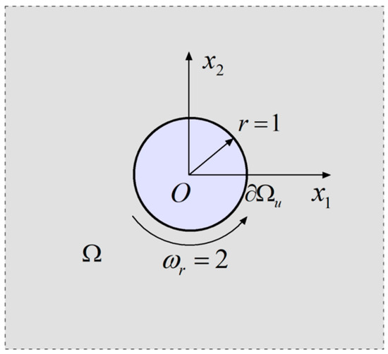
Figure 2. Rotating cylinder in an infinite domain.

The analytical solutions of the velocity field in this case are:

$$u_1(\mathit{x})=-\frac{2x_2}{x_1^2+x_2^2}, u_1(\mathit{x})=\frac{2x_1}{x_1^2+x_2^2}, \mathrm{in} \mathsf{\Omega }=\frac{{ℝ}^2}{||\mathit{x}||=1},$$

(61)

which gives $\mathsf{\Psi }=-2\ln ||\mathit{x}||$.

To verify the effectiveness of the proposed approaches for field value reconstruction, we corrupt the boundary data in Equation (60) by injecting white noise $w$ as:

$${\overline{u}}_1=-(2+w)\sin \theta , {\overline{u}}_2=(2+w)\cos \theta , \mathrm{on} \partial {\mathsf{\Omega }}_u.$$

(62)

where $w$ satisfies a Gaussian probability distribution of $p(w)=N(0,0.25{\omega }_r^2)=N(0,1)$.

In this case, we first simulated 80 distinct solutions of the velocity field under the noisy condition of Equation (62) by solving the interpolation equation Equation (34) with MFS. The velocities on axis x1 with $x_1=$ 1.01, 5, 10, 20, and 40 were reconstructed using a Kalman filter. In the field value reconstruction, the process noise covariance was $\mathit{Q}=0.01$, measurement noise covariance was $\mathit{R}=0.001$ and the initial estimate covariance was ${\mathit{P}}_0=0.01$. The state transition and transformation matrices are $\mathit{B}=\mathit{H}=\mathit{I}\in {ℝ}^{10\times 10}$. The vectors of the initial guess and measurement are calculated:

$${\widehat{\mathit{X}}}_0=[10,10,10,10,10,10,10,10,10,10], {\mathit{Z}}_k=[u^T(1.01,0),u^T(5,0),u^T(10,0),u^T(20,0)],$$

which is from 80 corrupted data (noisy values).

For simplicity, we only give the velocity reconstruction process of a Kalman filter at the location (1.01, 0) as shown in Figure 3 and Figure 4. In Figure 3 and Figure 4, it is shown that the filter estimates $u_i(1.01,0)$ ($i=1,2$) are convergent to the real states (analytical solutions) at the iteration step $k\approx 20$ with high speeds and strong robustness.

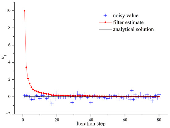
Figure 3. The reconstruction process of $u_1$ at (1.01, 0).

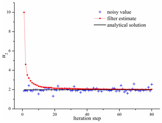
Figure 4. The reconstruction process of $u_2$ at (1.01, 0).

The final filter estimate and MFS solution under normal boundary conditions at the specific locations are compared with the analytical solution in Table 1. From Table 1, one can see that the MFS results have high accuracy about machine precision, and the maximum relative error of filtering values is about 5.0%.

Table 1. The reconstructed velocity fields $u_2$ and $u_1$ in exterior problem compared to MFS solutions and analytical solutions.

Location	Filter Estimate		MFS Result		Analytical Solution
	$${\mathit{u}}_2$$	$${\mathit{u}}_1$$	$${\mathit{u}}_2$$	$${\mathit{u}}_1$$	$${\mathit{u}}_2$$	$${\mathit{u}}_1$$
(1.01, 0.00)	2.022531	0.023287	1.980198	1.388 × 10−17	1.980198	0.000000
(5.00, 0.00)	0.408934	0.021637	0.400000	1.683 × 10−16	0.400000	0.000000
(10.00, 0.00)	0.207346	0.018830	0.200000	6.590 × 10−16	0.200000	0.000000
(20.00, 0.00)	0.105013	0.016672	0.100000	2.153 × 10−16	0.100000	0.000000
(40.00, 0.00)	0.052303	0.014703	0.050000	3.990 × 10−16	0.050000	0.000000

The velocities $u_1$ and $u_2$ on axis $x_1$ as obtained by the Kalman filter are shown in Figure 5, compared to those given by MFS and analytical solution. Figure 5 illustrates again that the MFS results have are highly accurate and the filter estimates agree well with the analytical solution. We conclude that the approach to an exterior problem presented in this paper is valid, and the Kalman filter is effective for the noisy boundary conditions.

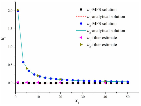
Figure 5. The velocities $u_2$ and $u_1$ along axis x1 based on Kalman filter, MFS and analytical solution.

5.1.2. Interior Problem with Mixed Boundary Conditions

The second numerical experiment was performed on $\mathsf{\Omega }=[-5,5]\times [-5,5]\cap ||x||\ge 1$ as shown in Figure 6, with an analytical solution [7]:

$$u_1(\mathit{x})=\frac{2x_1\left(x_1^2-x_2^2\right)}{{\left(x_1^2+x_2^2\right)}^2}, u_2(\mathit{x})=\frac{2x_2\left(x_1^2-x_2^2\right)}{{\left(x_1^2+x_2^2\right)}^2}, p(\mathit{x})=\frac{4\left(x_1^2-x_2^2\right)}{{\left(x_1^2+x_2^2\right)}^2}, \mathrm{in} \mathsf{\Omega },$$

(63)

for which one gets $\mathsf{\Psi }=2x_1{x}_2/{(x_1^2+x_2^2)}^2$.

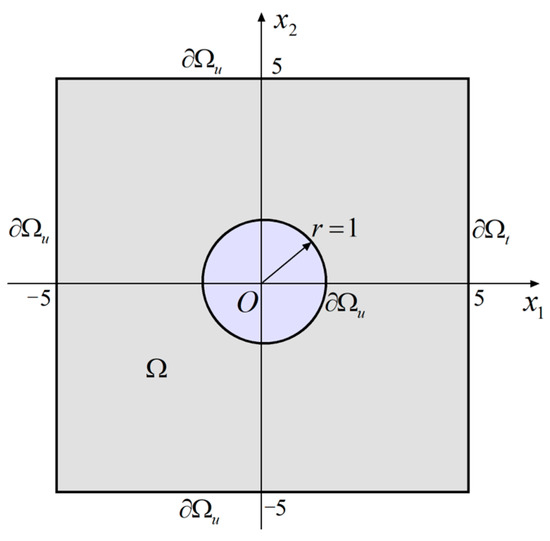
Figure 6. An interior Stokes problem of mixed boundary conditions.

In this case, the mixed boundary conditions are considered with $\partial {\mathsf{\Omega }}_t$ on $x_1=5$ and $\partial {\mathsf{\Omega }}_u$ on the other boundaries, according to Equation (63). The approximate solutions of velocity and pressure can be calculated by MFS with the interpolation equation Equation (29). Similar to the last numerical experiment, we seeded 80 distinct solutions of velocity and pressure for field value reconstructions by corrupting the boundary data with white noise $w$ with a Gaussian probability distribution of $p(w)=N(0,2)$. The velocities and pressures on axis $x_1$ at the locations $x_1=$ 1.01, 1.5, 2.5, 3.5, 4.5, and 4.99 have been reconstructed by the Kalman filter. It is noted that the process noise covariance $\mathit{Q}$, measurement noise covariance $\mathit{R}$, and initial estimate covariance ${\mathit{P}}_0$ are the same as those in the last numerical experiment. The state transition and transformation matrices are $\mathit{B}=\mathit{H}=\mathit{I}\in {ℝ}^{12\times 12}$ for the velocity fields and $\mathit{B}=\mathit{H}=\mathit{I}\in {ℝ}^{6\times 6}$ for the pressure fields. The vector of measurement for velocity and pressure are given by:

$${\mathit{Z}}_k={[{\mathit{u}}^T(1.01,0),{\mathit{u}}^T(1.5,0),{\mathit{u}}^T(2.5,0),{\mathit{u}}^T(3.5,0),{\mathit{u}}^T(4.5,0),{\mathit{u}}^T(4.99,0)]}^T,$$

and

$${\mathit{Z}}_k={[p(1.01,0),p(1.5,0),p(2.5,0),p(3.5,0),p(4.5,0),p(4.99,0)]}^T,$$

with both initial guesses ${\widehat{\mathit{X}}}_0=10$.

Figure 7, Figure 8 and Figure 9 depict the Kalman iteration processes for $u_1$, $u_2$, and $p$ at the location (1.01, 0). One can see that these estimates converge quickly to the real states. It is also found that pressures corrupted by noisy boundary data are more sensitive than velocities. Table 2 and Table 3 compare the filter estimates of velocity and pressure at specified locations with the MFS results and analytical solutions. It is illustrated that the filter estimates for velocity fields have a maximum relative error of about 4%, and those for pressure fields have a maximum relative error of about 9.5%, both of which are induced by the wider dispersed noised pressure data.

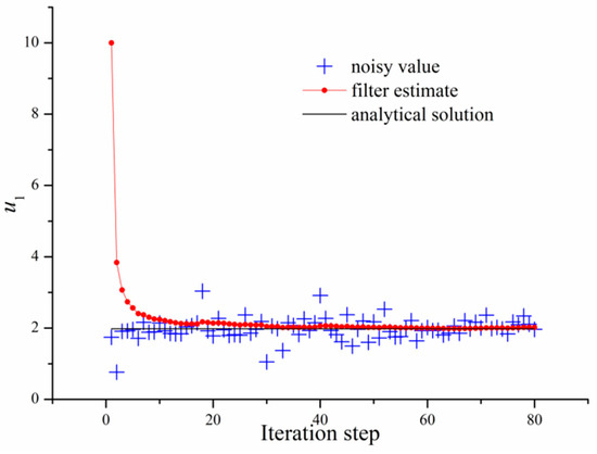
Figure 7. The reconstruction process of $u_1$ ($\mathit{x}=(1.01,0)$).

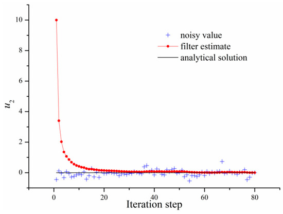
Figure 8. The reconstruction process of $u_2$ ($\mathit{x}=(1.01,0)$).

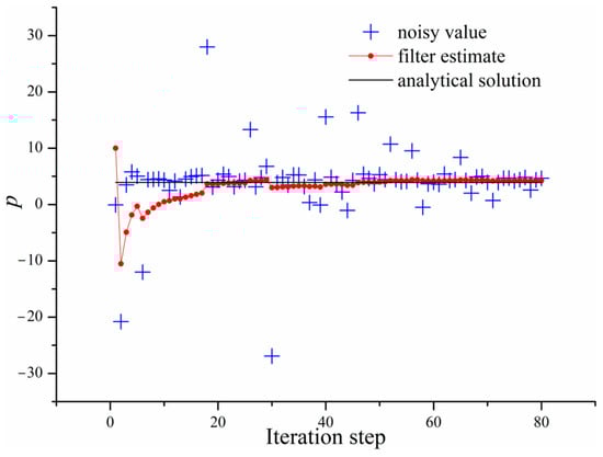
Figure 9. The reconstruction process of $p$ ($\mathit{x}=(1.01,0)$).

Table 2. The reconstructed velocity fields $u_2$ and $u_1$ in interior problem compared to MFS solutions and analytical solutions.

Location	Filter Estimate		MFS Result		Analytical Solution
	$${\mathit{u}}_2$$	$${\mathit{u}}_1$$	$${\mathit{u}}_2$$	$${\mathit{u}}_1$$	$${\mathit{u}}_2$$	$${\mathit{u}}_1$$
(1.01, 0.00)	0.002786	2.019726	2.891 × 10−13	1.980198	0.000000	1.980198
(1.50, 0.00)	0.002519	1.424964	2.340 × 10−12	1.333333	0.000000	1.333333
(2.50, 0.00)	−0.018299	0.859495	4.684 × 10−12	0.800000	0.000000	0.800000
(3.50, 0.00)	−0.031648	0.604543	5.976 × 10−12	0.571429	0.000000	0.571429
(4.50, 0.00)	−0.038981	0.458600	5.277 × 10−12	0.444444	0.000000	0.444444
(4.99, 0.00)	−0.037578	0.407153	3.630 × 10−12	0.400802	0.000000	0.400802

Table 3. The reconstructed pressure field $p$ compared to MFS solutions and analytical solutions.

Location	Filter Estimate	MFS Result	Analytical Solution
(1.01, 0.00)	4.216640	3.921184	3.921184
(1.50, 0.00)	1.951470	1.777778	1.777778
(2.50, 0.00)	0.668611	0.640000	0.640000
(3.50, 0.00)	0.325363	0.326531	0.326531
(4.50, 0.00)	0.187576	0.197531	0.197531
(4.99, 0.00)	0.150386	0.160642	0.160642

The distributions of velocities $u_1$, $u_2$ and pressure $p$ on axis $x_1$ are shown in Figure 10 and Figure 11. Those filter estimates agree well with the MFS result and the analytical solution.

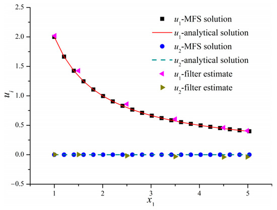
Figure 10. The velocities $u_1$, and $u_2$ along axis $x_1$ based on Kalman filter, MFS and the analytical solution.

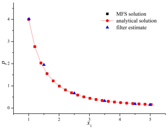
Figure 11. The pressure $p$ along axis $x_1$ based on Kalman filter, MFS and the analytical solution.

In the above two numerical experiments, one can see that the measurements severely corrupted by $\sqrt{1}$ and $\sqrt{2}$ root mean squared (RMS) noises, which are in the same magnitude as the boundary conditions. In spite of these high-level noises, the field values can be reconstructed with strong robustness. Therefore, it is concluded that the presented approach to field value reconstruction is valid for the noised boundary conditions.

5.2. Numerical Experiment for Velocity Identification

Consider a Stokes problem in the domain $\mathsf{\Omega }=r_r\le ||\mathit{x}||\le r_{\mathit{R}}$ with angular velocities ${\omega }_r$ and ${\omega }_R$ as shown in Figure 12. The analytical solutions for $\mathit{u}(\mathit{x})$ are:

$$u_1(\mathit{x})=\frac{C_1{x}_2}{x_1^2+x_2^2}+C_2{x}_2, u_2(\mathit{x})=-\frac{C_1{x}_1}{x_1^2+x_2^2}-C_2{x}_1, \mathrm{in} \mathsf{\Omega },$$

(64)

which gives $\mathsf{\Psi }=C_1\ln ||\mathit{x}||+C_2||\mathit{x}|{|}^2$, where:

$$C_1=\frac{({\omega }_r-{\omega }_R){(r_r{r}_R)}^2}{r_R^2-r_r^2}, C_2=\frac{{\omega }_r{r}_r^2-{\omega }_R{r}_R^2}{r_R^2-r_r^2}.$$

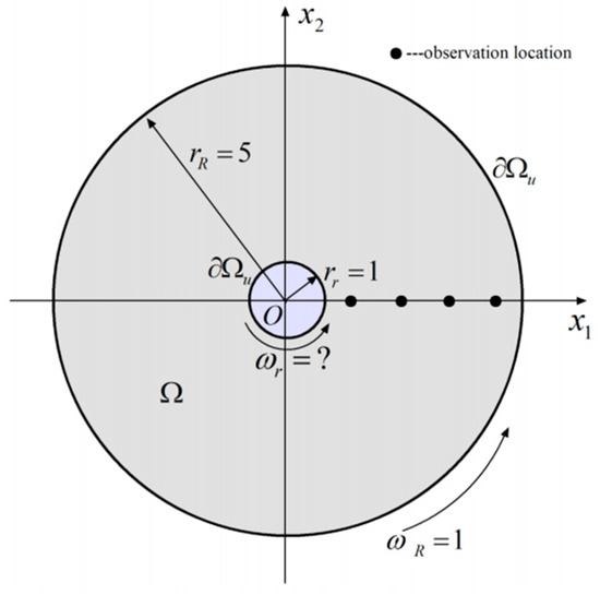
Figure 12. Stokes flow in the concentric cylinders for velocity identification.

We assumed that the angular velocity ${\omega }_r$ for inner cylinder ($r_r=1$) is unknown (to be identified with a real value ${\omega }_r=5$), and the angular velocity of outside hollow cylinder ($r_R=5$) was ${\omega }_R=1$, as shown in Figure 12. In this case, the additional observation velocities $\mathit{u}(\mathit{x})$ on axis $x_1$ at locations $x_1=$ 1.5, 2.5, 3.5, 4.5 were considered to identify the velocity. Firstly, the inverse problem was solved directly by Equation (54) with boundary node numbers $M$ = 48, 96, 192, and 384. It is found in Table 4 that the MFS results had relatively large errors of about 20%. The proposed approach to velocity identification in this paper was then applied to achieve the proper ${\omega }_r$. The addition noises $\mathit{w}$ were injected into the boundary conditions with a Gaussian probability distribution of $p(w)=N(0,0.0025)$. After 80 distinct corrupted solutions for ${\omega }_r$ were obtained, the Kalman filter with an initial guess of ${\omega }_r=50$ was applied to solve the unknown angular velocity. It is noted that the vectors of prediction and measurement degenerated to scalar with $B=H=1$. Furthermore, the process noise covariance $Q=1$, measurement noise covariance $R=0.01$, and initial estimate covariance $P_0=1$ were given in the Kalman filtering process.

Table 4. The reconstruction of ${\omega }_r$ compared to the MFS solution and analytical solution.

Boundary Node Number	Filter Estimate	MFS Result	Analytical Solution
48	4.801551	3.560083	5.000000
96	5.059094	4.052769	5.000000
192	5.101907	4.120948	5.000000
384	5.085097	4.095665	5.000000

From Table 4, it is seen that the filter estimates have better accuracies (with a maximum relative error of 2%) than those obtained by MFS. We also gave the iteration process of the Kalman filter with boundary node number $M=96$ as an example, which is depicted in Figure 13. It is seen in Figure 13 that the noised ${\omega }_r$ severely deviates from the real state, which implies that the interpolation Equation (54) is seriously ill-conditioned.

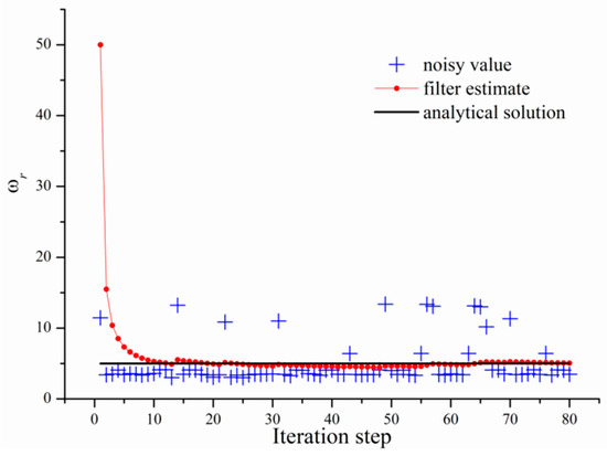
Figure 13. The iteration process of ${\omega }_r$ with noised data.

The velocities solved with the reconstructed ${\omega }_r$ by the Kalman filter along axis $x_1$ in domain $\mathsf{\Omega }$ are shown in Figure 14. It is seen that the approximate velocity fields agree well with the analytical solutions.

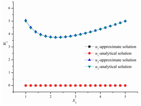
Figure 14. The approximate velocity fields with the reconstructed ${\omega }_r$ compared to analytical solutions.

5.3. Numerical Experiment for Dynamic Viscous Constant Identification

The last numerical experiment was performed to show the validation of applying the presented approach to dynamic viscous constant identification. Consider a Stokes problem in the domain $\mathsf{\Omega }=[-0.5,0.5]\times [-0.5,0.5]$ as shown in Figure 15. The analytical solutions for u are given by [7]:

$$u_1(\mathit{x})=-x_1^2+4x_2^3, u_2(\mathit{x})=4x_1^3+2x_1{x}_2-1, p(\mathit{x})=\frac{24x_1{x}_2-2x_1+1}{100} \mathrm{in} \mathsf{\Omega },$$

(65)

for which we define $\mathsf{\Psi }=-x_1^4+x_2^4-x_1^2{x}_2+x_1+1$.

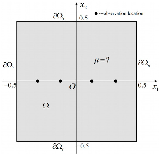
Figure 15. Stokes flow in a rectangle plate for dynamic viscous constant identification.

From Equations (5) and (65) one can see that the real dynamic viscous constant $\mu =0.01$. In this case, the four supplementary observation velocities $\mathit{u}(\mathit{x})$ on axis $x_1$ at locations $x_1=$ −0.3, −0.1, 0.1, 0.3 are given to identify the viscous constant. Similar to the last numerical experiment, the inverse problem is solved first using Equation (59) with boundary node numbers $M=$ 24, 48, 96, and 192. It is seen in Table 5 that the MFS results have a maximum relative error of about 1%. Thus, one can conclude that the dynamic viscous constant identification could be given directly by Equation (59) in this case. To reveal the robustness of the presented approach using a Kalman filter in this paper, we added the noises w to the boundary conditions with a Gaussian probability distribution of $p(w)=N(0,0.0002)$. The Kalman filter with initial guess $\mu =0.01$, was applied to solve the unknown viscous constant using 80 distinct corrupted solutions. We note that the vectors of prediction and measurement also degenerated to scalar with $B=H=1$. In the Kalman filtering iteration, the process noise covariance, measurement noise covariance, and initial estimate covariance were given the same value as the last numerical experiment.

Table 5. The reconstruction of $\mu$ compared to the MFS solution and analytical solution.

Boundary Node Number	Filter Estimate	MFS Result	Analytical Solution
24	0.010029	0.010002	0.010000
48	0.009878	0.009909	0.010000
96	0.010040	0.009958	0.010000
192	0.009771	0.010007	0.010000

Table 5 lists the filter estimates with different boundary numbers. It was found that these estimates had lower accuracies (about 3% maximum error) than those obtained directly by MFS. Figure 16 shows the convergence for a Kalman filter. One can see that the dynamic viscous constant’s estimate steadily trends toward the real value. The velocities $u_1$, $u_2$, and pressure $p$ utilizing the dynamic viscous constant obtained by a Kalman filter compared to the analytical solutions are shown in Figure 17 and Figure 18. Since the approximate pressure field offers higher accuracy, the two lines (approximate solution and analytical solution) in Figure 18 overlap each other. The velocity fields are slightly different from the analytical solution, which implies that the error of the viscous constant affects the velocities in some degree. It is emphasized that while the viscous constant identification could be obtained by applying a Kalman filter, the MFS may provide a more accurate solution.

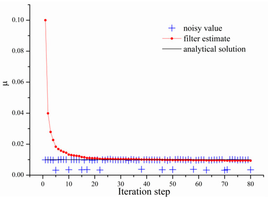
Figure 16. The iteration process of $\mu$ with noised data.

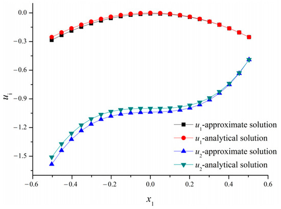
Figure 17. The approximate velocity fields with the reconstructed $\mu$ compared to analytical solutions.

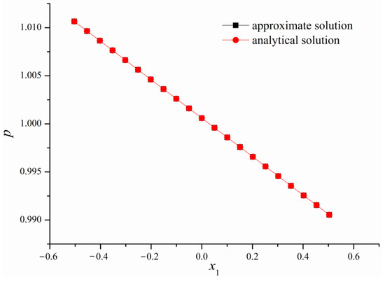
Figure 18. The approximate pressure field with the reconstructed $\mu$ compared to analytical solution.

6. Conclusions

Three types of inverse problems including field value reconstruction, velocity and dynamic viscous constant identifications were studied by applying the MFS and Kalman filter technique in this paper. Additionally, the equations to solve exterior (unbounded) problems of Stokes flow were derived by considering the boundary conditions as infinite. It is emphasized that the velocity and pressure at infinity should be uniform for unbounded problems, as mentioned before. The interpolation equations in Equations (54) and (59) were derived to solve the angular velocities and dynamic viscous constant by transforming the normal interpolation Equation (29) or (34) of MFS. To determine the optimal objective value, the Kalman filter technique was applied to solve the mentioned inverse problems by analyzing the discrete objective data obtained by injecting white noise with Gaussian distribution into the boundary conditions. Furthermore, the algorithms were presented to solve those inverse problems.

Four numerical experiments were given to show the high performance of the proposed approaches to the inverse problems. The first two numerical experiments revealed that the presented method has strong robustness and high accuracy in solving Stokes problems with noisy boundary conditions. The third numerical experiment proved that the proposed algorithm for angular velocity identification is powerful in solving this kind of inverse problem. The last numerical experiment showed that the present method could also determine the optimal dynamic viscous constant, although the MFS could directly solve that with relatively high accuracy.

The proposed approaches and algorithms for the mentioned inverse problems can be used for two-dimensional Stokes problems and can be extended to bounded three-dimensional problems. Additionally, it is noted that the velocity and pressure at infinity should be uniform for unbounded problems. Furthermore, it should be noted here that in this paper we only consider simple cases of the inverse Stokes problems, in which the geometric reconstruction and source identification are not concerns. The authors hope that the proposed approaches can be extended into these problems.

References

- Happel, J.; Brenner, H. Low Reynolds Number Hydrodynamics; Prentice-Hall: Englewood Cliffs, NJ, USA, 1965. [Google Scholar]
- Lin, J.; Yu, H. Simulation of antiplane shear problems with multiple inclusions using the generalized finite difference method. Appl. Math. Lett. 2021, 121, 107431. [Google Scholar] [CrossRef]
- Lin, J.; Yu, H.; Reutskiy, S.; Wang, Y. A meshless radial basis function based method for modeling dual-phase-lag heat transfer in irregular domains. Comput. Math. Appl. 2021, 85, 1–17. [Google Scholar] [CrossRef]
- Wang, L.H. Radial basis functions methods for boundary value problems: Performance comparison. Eng. Anal. Bound. Elem. 2017, 84, 191–205. [Google Scholar] [CrossRef]
- Lin, Z.; Wang, D.D.; Qi, D.; Deng, L. A Petrov-Galerkin finite element-meshfree formulation for multi-dimensional fractional diffusion equations. Comput. Mech. 2020, 66, 323–350. [Google Scholar] [CrossRef]
- Yi, S.; Yao, L.Q.; Cao, Y. A novel stratified interpolation of the element-free Galerkin method for 2d plane problems. Eng. Anal. Bound. Elem. 2015, 50, 459–473. [Google Scholar] [CrossRef]
- Li, X.L. Development of a meshless galerkin boundary node method for viscous fluid flows. Math. Comput. Simul. 2011, 82, 258–280. [Google Scholar] [CrossRef]
- Aleksidze, M.A. On approximate solutions of a certain mixed boundary value problem in the theory of harmonic functions. Differ. Equ. 1966, 2, 515–518. [Google Scholar]
- Kupradze, V.; Aleksidze, M. The method of functional equations for the approximate solution of certain boundary value problems. USSR Comput. Math. Math. Phys. 1964, 4, 82–126. [Google Scholar] [CrossRef]
- Jiang, Q.; Zhou, Z.D.; Chen, J.B.; Yang, F.P. The method of fundamental solutions for two-dimensional elasticity problems based on the airy stress function. Eng. Anal. Bound. Elem. 2021, 130, 220–237. [Google Scholar] [CrossRef]
- Jiang, Q.; Zhou, Z.D.; Yang, F.P. A new approach to solve the anti-plane crack problems by the method of fundamental solutions. Eng. Anal. Bound. Elem. 2022, 125, 284–298. [Google Scholar] [CrossRef]
- Cheng, A.H.; Hong, Y. An overview of the method of fundamental solutions—Solvability, uniqueness, convergence, and stability. Eng. Anal. Bound. Elem. 2020, 120, 118–152. [Google Scholar] [CrossRef]
- Wang, D.D.; Wang, J.; Wu, J. Arbitrary order recursive formulation of meshfree gradients with application to superconvergent collocation analysis of Kirchhoff plates. Comput. Mech. 2020, 65, 877–903. [Google Scholar] [CrossRef]
- Lin, J.; Chen, W.; Wang, F. A new investigation into regularization techniques for the method of fundamental solutions. Math. Comput. Simul. 2011, 81, 1144–1152. [Google Scholar] [CrossRef]
- Young, D.L.; Jane, S.; Fan, C.M.; Krishnan, M.; Tsai, C.C. The method of fundamental solutions for 2D and 3D Stokes flows. J. Comput. Phys. 2006, 211, 1–8. [Google Scholar] [CrossRef]
- Young, D.L.; Chen, C.; Fan, C.M.; Krishnan, M.; Tsai, C.C. Method of fundamental solutions for stokes flows in a rectangular cavity with cylinders. Eur. J. Mech. B Fluids 2005, 24, 703–716. [Google Scholar] [CrossRef]
- Alves, C.J.S.; Silvestre, A.L. Density results using stokeslets and a method of fundamental solutions for the stokes equations. Eng. Anal. Bound. Elem. 2004, 28, 1245–1252. [Google Scholar] [CrossRef]
- Young, D.L.; Wu, J.; Chiu, C.L. Method of fundamental solutions for stokes problems by the pressure-stream function formulation. J. Mech. 2008, 24, 137–144. [Google Scholar] [CrossRef]
- Karageorghis, A.; Lesnic, D.; Marin, L. The method of fundamental solutions for Brinkman flows. part I. exterior domains. J. Eng. Math. 2021, 126, 10. [Google Scholar] [CrossRef]
- Karageorghis, A.; Lesnic, D.; Marin, L. The method of fundamental solutions for Brinkman flows. part II. interior domains. J. Eng. Math. 2021, 127, 19. [Google Scholar] [CrossRef]
- Fan, C.M.; Li, H.H. Solving the inverse stokes problems by the modified collocation Trefftz method and Laplacian decomposition. Appl. Math. Comput. 2013, 219, 6520–6535. [Google Scholar] [CrossRef]
- Fan, J.; Di Cristo, M.; Jiang, Y.; Nakamura, G. Inverse viscosity problem for the Navier-Stokes equation. J. Math. Anal. Appl. 2010, 365, 750–757. [Google Scholar] [CrossRef]
- Karageorghis, A.; Lesnic, D.; Marin, L. A survey of applications of the MFS to inverse problems. Inverse Probl. Sci. Eng. 2011, 19, 309–336. [Google Scholar] [CrossRef]
- Kalman, R.E. A new approach to linear filtering and prediction problems. J. Basic Eng. 1960, 82D, 35–45. [Google Scholar] [CrossRef]
- Brown, R.G.; Hwang, P.Y.C. Introduction to Random Signals and Applied Kalman Filtering, 3rd ed.; John Wiley and Sons, Inc.: New York, NY, USA, 1997. [Google Scholar]
- Villenas, F.I.; Vargas, F.J.; Peters, A.A. A Kalman-based compensation strategy for platoons subject to data loss: Numerical and empirical study. Mathematics 2023, 11, 1228. [Google Scholar] [CrossRef]
- Zhang, Q.; Xu, Y.; Wang, X.; Yu, Z.; Deng, T. Real-Time wind field estimation and pitot tube calibration using an extended Kalman filter. Mathematics 2021, 9, 646. [Google Scholar] [CrossRef]
- Dogariu, L.M.; Paleologu, C.; Benesty, J.; Stanciu, C.L.; Oprea, C.C.; Ciochina, S. A Kalman Filter for multilinear forms and its connection with tensorial adaptive filters. Sensors 2021, 21, 3555. [Google Scholar] [CrossRef] [PubMed]
- Tamuly, P.; Chakraborty, A.; Das, S. Nonlinear finite element model updating using constrained unscented Kalman filter for condition assessment of reinforced concrete structures. J. Civil Struct. Health Monit. 2021, 11, 1137–1154. [Google Scholar] [CrossRef]
- Luo, J.N.; Li, X.L.; Xiong, Y.; Liu, Y. Groundwater pollution source identification using Metropolis-Hasting algorithm combined with Kalman filter algorithm. J. Hydrol. 2023, 626, 130258. [Google Scholar] [CrossRef]
- Xu, Y.; Hu, M.; Zhou, A.; Li, Y.; Gong, C. State of charge estimation for lithium-ion batteries based on adaptive dual Kalman filter. Appl. Math. Model. 2020, 77, 1255–1272. [Google Scholar] [CrossRef]
- Mumtaz, F.; Imran, K.; Bukhari, S.B.A.; Mehmood, K.K.; Abusorrah, A.; Shah, M.A.; Kazmi, S.A.A. A Kalman filter-based protection strategy for microgrids. IEEE Access 2022, 10, 73243–73256. [Google Scholar] [CrossRef]
- Revach, G.; Shlezinger, N.; Ni, X.Y.; Escoriza, A.L.; van Sloun, R.J.G.; Eldar, Y.C. KalmanNet: Neural network aided Kalman filtering for partially known dynamics. IEEE Trans. Signal Process. 2022, 70, 1532–1547. [Google Scholar] [CrossRef]
- Jiao, M.; Wang, D.; Yang, Y.; Liu, F. More intelligent and robust estimation of battery state-of-charge with an improved regularized extreme learning machine. Eng. Appl. Artif. Intell. 2021, 104, 104407. [Google Scholar] [CrossRef]
- Liu, S.; Yang, T.; Tang, M.; Wang, P.; Zhang, X. Suitable or optimal noise benefits in signal detection. Chaos Solitons Fractals 2016, 85, 84–97. [Google Scholar] [CrossRef]
- Rodriguez-Garcia, M.; Batet, M.; SAnchez, D. A semantic framework for noise addition with nominal data. Knowl.-Based Syst. 2017, 122, 103–118. [Google Scholar] [CrossRef]
Disclaimer/Publisher’s Note: The statements, opinions and data contained in all publications are solely those of the individual author(s) and contributor(s) and not of MDPI and/or the editor(s). MDPI and/or the editor(s) disclaim responsibility for any injury to people or property resulting from any ideas, methods, instructions or products referred to in the content. |
© 2023 by the authors. Licensee MDPI, Basel, Switzerland. This article is an open access article distributed under the terms and conditions of the Creative Commons Attribution (CC BY) license (https://creativecommons.org/licenses/by/4.0/).