
Scale Mixture of Exponential Distribution with an Application


 , ,
, ,  and
and 
Abstract
1. Introduction
2. Density Function and Properties
2.1. Scale Mixture
2.2. Properties
2.3. Cumulative Distribution Function
2.4. Reliability Analysis
- 1.
- 2.
2.5. Order Statistics
2.6. Moment-Generating Function and Moments
3. Inference
3.1. Moment Estimators
3.2. ML Estimators
3.3. Em Algorithm
- E-step: For , use , the estimate of at the -th iteration of the algorithm, to computewhereand corresponds to the pdf of the model.
- M1-step: Update as
- M2-step: Update as the solution for the non-linear equationwhere is the digamma function and and denote the mean of and evaluated in the k-th step, respectively.
3.4. Observed Information Matrix
3.5. Simulation Study
| Algorithm 1 Algorithm to simulate values from the distribution. |
|
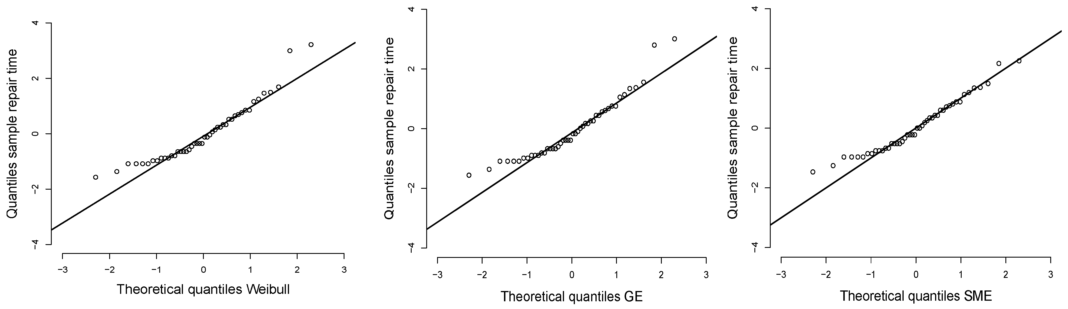
4. Application
5. Conclusions
- The SME distribution has two representations, given in (1) and in Proposition 1.
- Based on the mixed-scale representation, the SME distribution was implemented using the EM algorithm to calculate the maximum likelihood estimators.
- The simulation study shows that the ML estimators produce very good results with small samples.
- Our application shows that the SME distribution is a good option when the data have a heavy right tail; this is confirmed by the AIC and BIC model selection criteria in a comparison with the Weibull and GE distributions.
- We are working on an extension of the SME distribution that will have a more flexible mode, as well as using it to model data with covariables.
Supplementary Materials
Author Contributions
Funding
Institutional Review Board Statement
Informed Consent Statement
Data Availability Statement
Conflicts of Interest
Appendix A
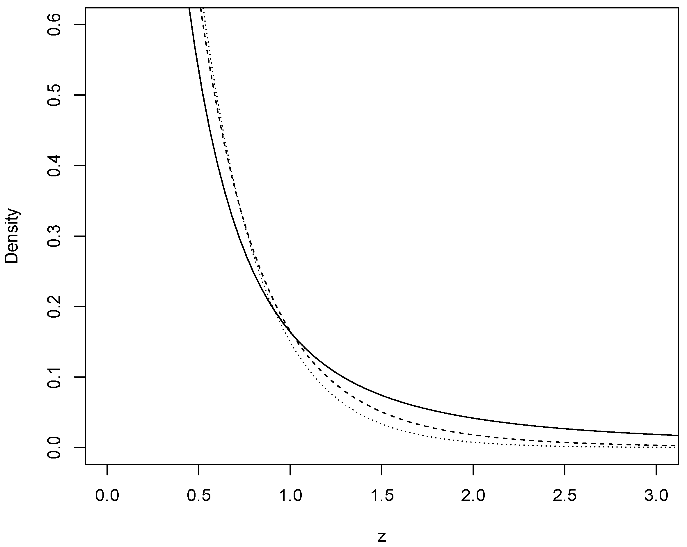
- Density function.The hypergeometric function contained in the CharFun package was used to obtain the graph of the density function.$eexp<-function(a,b1,b2,b3){x <- seq(0, 6, 0.04)y <- (a)*exp(-2*a*x)*hypergeom1F1(2*a*x,b1,2*b1+1)y1 <- (a)*exp(-2*a*x)*hypergeom1F1(2*a*x,b2,2*b2+1)y2 <- (a)*exp(-2*a*x)*hypergeom1F1(2*a*x,b3,2*b3+1)y3<- a*exp(-a*x)plot(x,y, type = "l",, ylim = c (0,0.6), xlim = c(0, 3), xlab="z",ylab="Density")lines(x, y1, lty = 2)lines(x, y2, lty = 3)lines(x, y3, lty = 4)}eexp(3,1,5,10)$
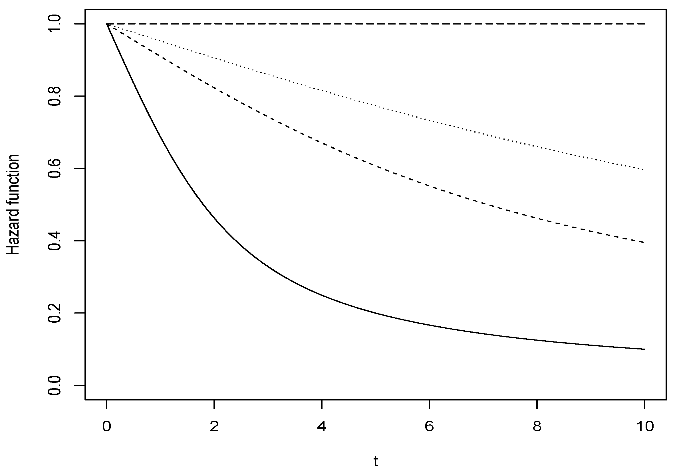
- Hazard functionThe hypergeometric function contained in the CharFun package was also used to obtain the graph of the hazard function.$hexp<- function(a,b1,b2,b3){x <- seq(0, 10, 0.04)y <- ((a)*hypergeom1F1(2*a*x,b1,2*b1+1))/(hypergeom1F1(2*a*x,b1,2*b1))y1 <- ((a)*hypergeom1F1(2*a*x,b2,2*b2+1))/(hypergeom1F1(2*a*x,b2,2*b2))y2 <- ((a)*hypergeom1F1(2*a*x,b3,2*b3+1))/(hypergeom1F1(2*a*x,b3,2*b3))y3 <- (a*exp(-a*x))/(exp(-a*x))plot(x,y, type = "l",, ylim = c (0,1), xlim = c(0, 10), xlab="t",ylab="Hazard function")lines(x, y1, lty = 2)lines(x, y2, lty = 3)lines(x, y3, lty = 5)}hexp(1,1,5,10)$
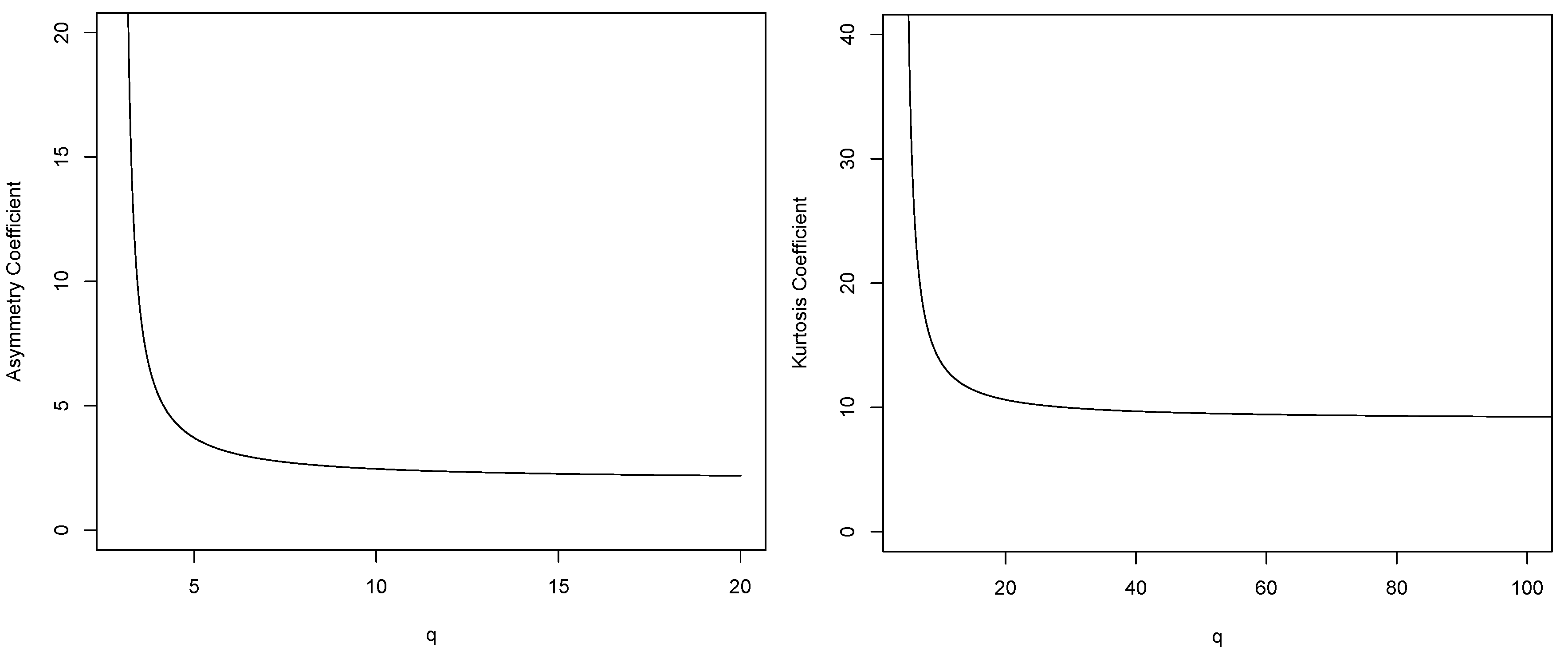
- Asymmetry Coefficient$q <- seq(3.01, 20.01, 0.01)b0 = beta(q,q)b1 = beta(q-1,q)b2 = beta(q-2,q)b3 = beta(q-3,q)Asym <- (2*(3*(b0)*b3-3*b0*b1*b2+b1))/(2*b0*b2-b1)(/2)plot(q,Asym, type = "l", ylim = c (0,20), xlab="q",ylab="Asymmetry Coefficient")$
- Kurtosis Coefficient$q <- seq(4.01, 140, 0.01)b0 = beta(q,q)b1 = beta(q-1,q)b2 = beta(q-2,q)b3 = beta(q-3,q)b4 = beta(q-4,q)Kurt <- (3*(8*b0*b4-8*b0*b1*b3+4*b0*b1*b2-b1))/(2*b0*b2-b1)()plot(q,Kurt, type = "l",xlim=c(5,100),ylim = c (0,40), xlab="q",ylab="Kurtosis Coefficient")$
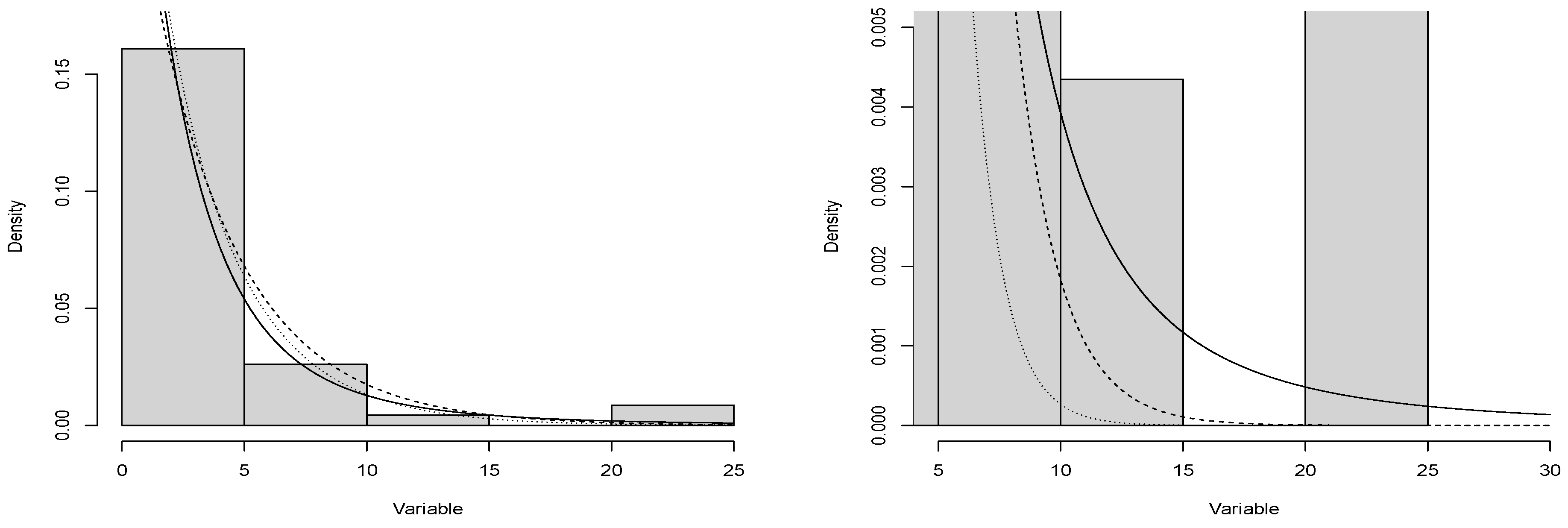
- ApplicationThe dataset, related to the repair time (hours) for a simple total sample of 46 airborne communications receivers:Parameter estimation using maximum likelihood estimators, to contrast the SME model with the Weibull and generalized exponential models:$#SMElibrary(CharFun)se3 <- function(theta){lambda = theta[1]q = theta[2]f = -log(lambda)-log(hypergeom1F1(-2*lambda*y,q+1,2*q+1))log.f = sum(f)return(log.f)}#Iterative Methodoptim(par=c(0.1067734,4),se3, hessian=TRUE, method="L-BFGS-B",lower=c(0,0),upper=c(Inf,Inf))n = optim(par=c(0.1067734,4),se3, hessian=TRUE, method="L-BFGS-B",lower=c(0,0),upper=c(Inf,Inf))#Hessian matrixsolve(n$hessian)#Standar Errorsqrt(round(diag(solve(n$hessian)),5))$$#Weibullse4 <- function(theta){lambda = theta[1]q = theta[2]f = -log(lambda)- log(q)-(q-1)*log(y)+lambda*ylog.f = sum(f)return(log.f)}#Iterative Methodoptim(par=c(0.106,2),se4, hessian=TRUE,method="L-BFGS-B",lower=c(0,0),upper=c(Inf,Inf))n = optim(par=c(0.106,2),se4, hessian=TRUE,method="L-BFGS-B",lower=c(0,0),upper=c(Inf,Inf))#Hessian matrixsolve(n$hessian)#Standar Errorsqrt(round(diag(solve(n$hessian)),5))$$#GEse5 <- function(theta){lambda = theta[1]q = theta[2]f = -log(q)-log(lambda)-(q-1)*log(1-exp(-lambda*y))+lambda*ylog.f = sum(f)return(log.f)}#Iterative Methodoptim(par=c(0.5268,0.7904),se5, hessian=TRUE, method="L-BFGS-B",lower=c(0,0),upper=c(Inf,Inf))n = optim(par=c(0.5268,0.7904),se5, hessian=TRUE, method="L-BFGS-B",lower=c(0,0),upper=c(Inf,Inf))#Hessian matrixsolve(n$hessian)#Standar Errorsqrt(round(diag(solve(n$hessian)),5))$$library(CharFun)hist(x, freq=F, ylim= c(0,0.17),ylab="Density", xlab="Variable", main="")#SME, values obtained by fitting the model:a1= 0.3722b1= 2.3078curve((a1)*exp(-2*a1*x)*hypergeom1F1(2*a1*x,b1,2*b1+1), add=T)#GE, values obtained by fitting the model:a2= 0.2694b2= 0.9583curve((b2)*(a2)*(1-exp(-x*a2))(2-1)*(exp(-x*a2)), lty = 2, add=T)#Weibull, values obtained by fitting the model:a3= 0.3337b3= 0.8986curve(a3*b3*((x*a3)(3-1))*exp(-x*a3)(3),lty=3, add=T)$$# QQPLOTS#WEIBULLdatos = xlambda= 0.3337q= 0.8986Fx= 1 - exp(-lambda*datos)f= qnorm(Fx)library(nortest)qqnorm(f, pch = 1, frame = FALSE,ylim=c(-4,4),xlim=c(-3,3),main="",cex.lab=1.5,cex.main=2,xlab="Theoretical quantiles Weibull",ylab="Quantiles sample repair time")qqline(f, col = "black", lwd = 2)$$#GEdatos = xlambda= 0.2694q= 0.9582Fx= (1 - exp(-lambda*datos))f= qnorm(Fx)library(nortest)qqnorm(f, pch = 1, frame = FALSE,ylim=c(-4,4),xlim=c(-3,3),main="",cex.lab=1.5,cex.main=2,xlab="Theoretical quantiles GE",ylab="Quantiles sample repair time")qqline(f, col = "black", lwd = 2)$$#SMElibrary(CharFun)datos = xlambda= 0.3722q= 2.3078Fx= 1-exp(-2*lambda*datos)*hypergeom1F1(2*lambda*datos,q,2*q)f= qnorm(Fx)library(nortest)qqnorm(f, pch = 1, frame = FALSE,ylim=c(-4,4),xlim=c(-3,3),main="",cex.lab=1.5,cex.main=2,xlab="Theoretical quantiles SME",ylab="Quantiles sample repair time")qqline(f, col = "black", lwd = 2)$
References
- Andrews, D.F.; Mallows, C.L. Scale Mixtures of Normal Distributions. J. R. Stat. Soc. Ser. B (Methodol.) 1974, 36, 99–102. [Google Scholar] [CrossRef]
- Fernández, C.; Steel, M.F. Bayesian Regression Analysis with Scale Mixtures of Normals. Econom. Theory 2000, 16, 80–101. [Google Scholar] [CrossRef]
- Johnson, N.L.; Kotz, S.; Balakrishnan, N. Continuous Univariate Distributions, 2nd ed.; Wiley: New York, NY, USA, 1995; Volume 1. [Google Scholar]
- Rogers, W.H.; Tukey, J.W. Understanding some long-tailed symmetrical distributions. Stat. Neerl. 1972, 26, 211–226. [Google Scholar] [CrossRef]
- Mosteller, F.; Tukey, J.W. Data Analysis and Regression; Addison-Wesley: Reading, MA, USA, 1977. [Google Scholar]
- Kadafar, K. A biweight approach to the one-sample problem. J. Am. Statist. Assoc. 1982, 77, 416–424. [Google Scholar] [CrossRef]
- Wang, J.; Genton, M.G. The multivariate skew-slash distribution. J. Stat. Plann. Inference 2006, 136, 209–220. [Google Scholar] [CrossRef]
- Olmos, N.M.; Varela, H.; Bolfarine, H.; Gómez, H.W. An extension of the generalized half-normal distribution. Stat. Pap. 2014, 55, 967–981. [Google Scholar] [CrossRef]
- Rivera, P.; Barranco-Chamorro, I.K.; Gallardo, D.I.; Gómez, H.W. Scale Mixture of Rayleigh Distribution. Mathematics 2020, 8, 1842. [Google Scholar] [CrossRef]
- Castillo, J.; Gaete, K.; Muñoz, H.; Gallardo, D.I.; Bourguignon, M.; Venegas, O.; Gómez, H.W. Scale Mixture of Maxwell-Boltzmann Distribution. Mathematics 2023, 11, 529. [Google Scholar] [CrossRef]
- Gupta, R.D.; Kundu, D. Generalized Exponential Distributions. Aust. N. Z. J. Stat. 1999, 41, 173–188. [Google Scholar] [CrossRef]
- Gupta, R.D.; Kundu, D. Exponentiated Exponential Family: An Alternative to Gamma and Weibull Distributions. Biom. J. 2001, 43, 117–130. [Google Scholar] [CrossRef]
- Gupta, R.D.; Kundu, D. Generalized exponential distribution: Existing results and some recent developments. J. Stat. Plann. Inference 2007, 137, 3537–3547. [Google Scholar] [CrossRef]
- Mudholkar, G.S.; Srivastava, D.K.; Freimer, M. The exponentiated Weibull Family—A reanalysis of the Bus-Motor-Failure data. Technometrics 1995, 37, 436–445. [Google Scholar] [CrossRef]
- Abramowitz, M.; Stegun, I.A. Handbook of Mathematical Functions with Formulas, Graphs, and Mathematical Tables, 9th ed.; National Bureau of Standards: Washington, DC, USA, 1970. [Google Scholar]
- R Core Team. R: A Language and Environment for Statistical Computing; R Foundation for Statistical Computing: Vienna, Austria, 2022; Available online: https://www.R-project.org/ (accessed on 12 January 2023).
- Dempster, A.P.; Laird, N.M.; Rubin, D.B. Maximum likelihood from incomplete data via the EM algorithm (with discussion). J. R. Stat. Soc. B Stat. Methodol. 1977, 39, 1–38. [Google Scholar]
- Gordy, M. A Generalization of Generalized Beta Distributions; Finance and Economics Discussion Series (FEDS); Board of Governors of the Federal Reserve System: Washington, DC, USA, 1998; p. 28. [Google Scholar]
- Devore, J.L. Probabilidad y Estadística para Ingeniería y Ciencias, 7th ed.; Cengage Learning Editores: Santa Fe, México, 2008. [Google Scholar]
- Akaike, H. A new look at the statistical model identification. IEEE Trans. Autom. Control 1074, 19, 716–723. [Google Scholar] [CrossRef]
- Schwarz, G. Estimating the dimension of a model. Ann. Stat. 1978, 6, 461–464. [Google Scholar] [CrossRef]


| Distribution | |||
|---|---|---|---|
| E(3) | |||
| SME(3,5) | |||
| SME(3,1) |
| True Value | Esti-Mator | ||||||||||||||||
|---|---|---|---|---|---|---|---|---|---|---|---|---|---|---|---|---|---|
| Bias | Relat. Bias | SE | RMSE | CP | Bias | Relat. Bias | SE | RMSE | CP | Bias | Relat. Bias | SE | RMSE | CP | |||
| 0.3 | 0.9 | 0.0056 | 0.0187 | 0.0699 | 0.0713 | 0.930 | 0.0012 | 0.0013 | 0.0478 | 0.0491 | 0.933 | 0.0003 | 0.001 | 0.0336 | 0.0335 | 0.935 | |
| q | 0.3494 | 0.3882 | 0.9341 | 1.5762 | 0.986 | 0.1436 | 0.1595 | 0.2650 | 0.3092 | 0.976 | 0.1114 | 0.1238 | 0.1717 | 0.2109 | 0.972 | ||
| 3 | 3 | 0.0578 | 0.0193 | 0.6108 | 0.6023 | 0.9480 | 0.0155 | 0.0052 | 0.4190 | 0.4122 | 0.9550 | −0.0048 | 0.0016 | 0.2940 | 0.3008 | 0.9400 | |
| q | 3.4563 | 1.1521 | 15.3985 | 7.6745 | 0.9320 | 2.2172 | 0.7391 | 7.5971 | 5.5487 | 0.9380 | 1.1422 | 0.3807 | 3.0497 | 3.4228 | 0.9480 | ||
| 5 | 0.0656 | 0.0131 | 1.0062 | 1.0137 | 0.9530 | 0.0428 | 0.0086 | 0.7028 | 0.7170 | 0.9430 | −0.0194 | 0.0039 | 0.4879 | 0.4872 | 0.9490 | ||
| q | 3.6878 | 0.7376 | 16.7017 | 7.8837 | 0.9260 | 2.5917 | 0.5183 | 8.8779 | 6.0848 | 0.9310 | 1.3019 | 0.2604 | 3.3514 | 3.7521 | 0.9400 | ||
| 10 | 0.1409 | 0.0469 | 2.0204 | 1.9723 | 0.9550 | 0.0725 | 0.015 | 1.3981 | 1.3559 | 0.9530 | 0.0022 | 0.0004 | 0.9789 | 1.0040 | 0.9310 | ||
| q | 3.4013 | 0.3401 | 15.5562 | 7.5771 | 0.9220 | 2.2612 | 0.2261 | 7.6449 | 5.8702 | 0.9290 | 1.0582 | 0.1058 | 2.9019 | 3.3276 | 0.9430 | ||
| 5 | 3 | 0.5401 | 0.1080 | 4.0908 | 4.1705 | 0.9460 | −0.1251 | 0.0250 | 2.7644 | 2.7372 | 0.9450 | −0.0381 | 0.0076 | 1.9573 | 1.9689 | 0.9460 | |
| q | 3.0615 | 1.0205 | 14.2999 | 7.1274 | 0.9040 | 2.4105 | 0.8035 | 8.1781 | 5.8233 | 0.9300 | 1.3798 | 0.4599 | 3.5320 | 4.0312 | 0.9400 | ||
| 5 | 0.1377 | 0.0275 | 0.6026 | 0.6105 | 0.9630 | 0.0458 | 0.0091 | 0.4117 | 0.4101 | 0.9510 | 0.0086 | 0.0017 | 0.2875 | 0.2837 | 0.9560 | ||
| q | 4.8173 | 0.9635 | 26.9415 | 9.7030 | 0.8810 | 3.9440 | 0.7888 | 16.6657 | 8.3701 | 0.9080 | 3.0671 | 0.6134 | 10.2178 | 7.1131 | 0.9220 | ||
| 10 | 0.2087 | 0.0417 | 1.0104 | 0.9979 | 0.9560 | 0.0768 | 0.0154 | 0.6851 | 0.6647 | 0.9550 | 0.0151 | 0.0030 | 0.4802 | 0.4748 | 0.9520 | ||
| q | 4.2450 | 0.4245 | 24.4946 | 9.0333 | 0.8980 | 4.1595 | 0.4159 | 17.1904 | 8.6566 | 0.9000 | 3.1381 | 0.3138 | 10.2049 | 7.1001 | 0.9030 | ||
| 10 | 3 | 0.4606 | 0.0461 | 2.0441 | 2.0142 | 0.9680 | 0.1480 | 0.0148 | 1.3829 | 1.3759 | 0.9570 | 0.0471 | 0.0047 | 0.9623 | 0.8868 | 0.9650 | |
| q | 3.5127 | 1.1709 | 22.3145 | 8.2245 | 0.8870 | 3.5210 | 1.1737 | 16.1847 | 7.8978 | 0.8950 | 2.8765 | 0.9588 | 9.8766 | 6.7824 | 0.9110 | ||
| 5 | 0.7591 | 0.0759 | 4.0391 | 4.0866 | 0.9480 | 0.4594 | 0.0459 | 2.7810 | 2.7219 | 0.9670 | 0.0627 | 0.0063 | 1.9278 | 1.8641 | 0.9540 | ||
| q | 3.7836 | 0.7567 | 23.6827 | 8.4779 | 0.8870 | 3.4580 | 0.6916 | 15.8695 | 7.8824 | 0.8790 | 2.6302 | 0.5260 | 9.3693 | 6.5207 | 0.9130 | ||
| 10 | 0.1918 | 0.0192 | 0.6125 | 0.5804 | 0.9790 | 0.1042 | 0.0104 | 0.4105 | 0.3916 | 0.9710 | 0.0522 | 0.0052 | 0.2827 | 0.2557 | 0.9730 | ||
| q | 0.9445 | 0.0945 | 30.4273 | 8.2888 | 0.7910 | 2.1081 | 0.2108 | 25.0503 | 8.1708 | 0.8270 | 2.9984 | 0.2998 | 20.0941 | 8.1843 | 0.8650 | ||
| 20 | 3 | 0.3712 | 0.0186 | 1.0259 | 1.0111 | 0.9700 | 0.1785 | 0.0089 | 0.6829 | 0.6624 | 0.9660 | 0.0689 | 0.0034 | 0.4714 | 0.4493 | 0.9680 | |
| q | 1.2705 | 0.4235 | 31.9658 | 8.2947 | 0.7920 | 2.1267 | 0.7089 | 24.7954 | 8.2037 | 0.8370 | 2.8024 | 0.9341 | 20.0680 | 8.0424 | 0.8640 | ||
| 5 | 0.7195 | 0.0359 | 2.0535 | 1.9473 | 0.9800 | 0.3663 | 0.0183 | 1.3723 | 1.3197 | 0.9770 | 0.1801 | 0.0090 | 0.9479 | 0.9108 | 0.9650 | ||
| q | 0.9469 | 0.1894 | 31.0027 | 8.0842 | 0.7730 | 1.9417 | 0.3883 | 24.5047 | 8.2527 | 0.8380 | 2.5291 | 0.5058 | 19.3210 | 7.8358 | 0.8560 | ||
| 10 | 1.4028 | 0.0701 | 4.1200 | 4.1425 | 0.9780 | 0.6564 | 0.0328 | 2.7491 | 2.5917 | 0.9750 | 0.3397 | 0.0169 | 1.8977 | 1.7311 | 0.9750 | ||
| q | 0.5117 | 0.0512 | 30.4592 | 8.1053 | 0.7670 | 1.7915 | 0.1792 | 25.0760 | 8.0883 | 0.8290 | 2.6677 | 0.2668 | 20.1392 | 7.8305 | 0.8630 | ||
| n | ||||
|---|---|---|---|---|
| 46 | 3.607 | 24.445 | 2.795 | 8.295 |
| Parameters | Weibull | GE | SME |
|---|---|---|---|
| Estimate | Estimate | Estimate | |
| 0.3337 | 0.2694 | 0.3722 | |
| q | 0.8985 | 0.9582 | 2.3078 |
| Log-likelihood | −104.4697 | −104.9829 | −102.9231 |
| AIC | 212.9394 | 213.9658 | 209.8462 |
| BIC | 216.5967 | 217.6231 | 213.5035 |
Disclaimer/Publisher’s Note: The statements, opinions and data contained in all publications are solely those of the individual author(s) and contributor(s) and not of MDPI and/or the editor(s). MDPI and/or the editor(s) disclaim responsibility for any injury to people or property resulting from any ideas, methods, instructions or products referred to in the content. |
© 2024 by the authors. Licensee MDPI, Basel, Switzerland. This article is an open access article distributed under the terms and conditions of the Creative Commons Attribution (CC BY) license (https://creativecommons.org/licenses/by/4.0/).
Share and Cite
Barahona, J.A.; Gómez, Y.M.; Gómez-Déniz, E.; Venegas, O.; Gómez, H.W. Scale Mixture of Exponential Distribution with an Application. Mathematics 2024, 12, 156. https://doi.org/10.3390/math12010156
Barahona JA, Gómez YM, Gómez-Déniz E, Venegas O, Gómez HW. Scale Mixture of Exponential Distribution with an Application. Mathematics. 2024; 12(1):156. https://doi.org/10.3390/math12010156
Chicago/Turabian StyleBarahona, Jorge A., Yolanda M. Gómez, Emilio Gómez-Déniz, Osvaldo Venegas, and Héctor W. Gómez. 2024. "Scale Mixture of Exponential Distribution with an Application" Mathematics 12, no. 1: 156. https://doi.org/10.3390/math12010156
APA StyleBarahona, J. A., Gómez, Y. M., Gómez-Déniz, E., Venegas, O., & Gómez, H. W. (2024). Scale Mixture of Exponential Distribution with an Application. Mathematics, 12(1), 156. https://doi.org/10.3390/math12010156