University Campus as a Complex Pedestrian Dynamic Network: A Case Study of Walkability Patterns at Texas Tech University ^†

Abstract

Statistical mechanics of walks defined on the spatial graphs of the city of Lubbock (10,421 nodes) and the Texas Tech University (TTU) campus pedestrian network (1466 nodes) are used for evaluating structural isolation and the integration of graph nodes, assessing their accessibility and navigability in the graph, and predicting possible graph structural modifications driving the campus evolution. We present the betweenness and closeness maps of the campus, the first passage times to the different campus areas by isotropic and anisotropic random walks, as well as the first passage times under the conditions of traffic noise. We further show the isolation and integration indices of all areas on the campus, as well as their navigability and strive scores, and energy and fugacity scores. The TTU university campus, a large pedestrian zone located close to the historical city center of Lubbock, mediates between the historical city going downhill and its runaway sprawling body.

1. Introduction—Walkability in a Campus Pedestrian Network

The rapid urbanization and widespread use of cars have resulted in a decline in walking as a primary mode of transportation [1]. Modern American cities offer very limited opportunities for safe walking. Moreover, a person walking outside an urban park or a recreational area may appear quite suspicious and, as a result, immediately attract police attention. However, in downtown city areas, there is a growing public preference for walking as a means to promote active and healthy lifestyles, while also addressing challenges such as air pollution and traffic congestion [1,2].

The physical environment of a university campus provides American students with a rare, if not unique, opportunity to experience walking not only as the most natural mode of transportation but also as a culture that positively impacts cognitive functions like creativity, memory, and concentration [1,3]. It also improves community health by promoting social interactions, economic aspects, and environmental impact [3,4,5].

Walkability is a complex concept involving many factors such as proximity, convenience, safety, and comfort for walkers [6]. Urban forms can encourage or hinder walking activity and, therefore, have a direct impact on accessibility to different places in the built environment. However, the relationship between urban form and walking patterns may show significant differences among different population subgroups, for instance, in terms of gender [1].

For college students, walkability is crucial as it serves as their main daily transportation mode and aids in achieving physical activity goals. University campuses comprising buildings, outdoor spaces, and support elements, akin to mini-cities, require well-designed pedestrian pathways for overall efficiency [7,8]. The campus serves as a pivotal aspect of students’ college experiences, hosting diverse activities [9] and offering various amenities that promote active lifestyles, influencing students’ physical activity patterns and travel behavior [10]. The presence of pedestrian-friendly pathways adhering to established norms and promoting overall functionality and sustainability, plays a vital role in facilitating student mobility and connecting key destinations within the campus environment, such as parking lots, bus stops, lecture halls, libraries, and offices. A walkable campus enhances accessibility, reduces vehicle reliance, improves air quality, and fosters a vibrant social atmosphere. Conversely, a dispersed plan hinders walkability, leading to challenges like increased vehicle use, reduced energy efficiency, and limited social interactions [2]. Among the various types of open spaces, streets serve as essential public realms for students to socialize and engage in daily activities. Studies suggest that visually appealing and comfortable streets can encourage physical activities among students on campus [11].

In our work, we study the spatial morphology of a campus pedestrian network (CPN) comprising 1466 interconnected walkable spaces identified in situ at the Texas Tech University (TTU) campus located in Lubbock, Texas. Pedestrian networks within an urban space include interconnected walkways, sidewalks, crosswalks, pedestrian signals, and other features that are designed to facilitate pedestrian movement. In the city, they provide safe and convenient access to important destinations, such as schools, parks, shopping centers, and public transportation hubs [12]. With the use of statistical mechanics of walks defined on the spatial graph representing the pedestrian network, we rigorously define and evaluate the important walkability characteristics, such as isolation, integration, accessibility, and navigability of all places (morphemes) in the CPN.

Cities are often likened to living organisms that must constantly evolve to efficiently manage our communications and adapt to the growing intensity of our daily activities. The spatial configuration of cities plays a key role in generating movement and attracting diverse land uses [13]. Urban morphology, which focuses on the scientific examination of forms, geometries, and configurations within cities, is crucial in assessing the transportation capacity and walkability of urban environments. Indeed, our daily experiences of moving in the city show that street blockages, traffic incidents, and random roadway repairs often lead to immediate and unpredictable dramatic changes in the usual traffic and pedestrian flows, sometimes affecting areas tens of miles from the place. Vehicle drivers choose alternative routes to avoid potential traffic jams on congested roads, and pedestrians alter their usual walking routes to steer clear of construction zones and areas that seem unpleasant or dangerous to walk through. The spontaneous choice of new paths is largely influenced by chance and is often predetermined by the urban structure. Natural movement theory suggests that people are drawn to highly integrated or connected streets and dense commercial destinations. Moreover, land use itself can increase movement through a multiplier effect by attracting more pedestrians to densely connected streets and bustling commercial areas [14]. Morphology involves identifying patterns of movement and studying the arrangements of buildings and related walking spaces. Urban design aims to create intentional movement patterns by developing the relevant urban space.

Walkability refers to the ease and convenience of walking within an urban environment, and it is closely tied to urban morphology, which is the physical structure and layout of the city and, therefore, comprehending urban morphology is essential to enhance walkability and improve the quality of urban life [6]. Walkability studies conducted on university and college campuses or communities with schools can be classified into two main approaches. The first method involves measuring the walkability of existing environments, which can further be divided into units of analysis, such as campus layout, street network organization, and path segments. Various tools are utilized for morphological analysis, including walk scores, surveys, sketch maps, interviews, audits, participatory tools, video recordings, reports, and pedometers. The analysis methods can either focus on quantitative data related to the environment’s characteristics (e.g., the density of people or buildings, intersection density, street connectivity, and sidewalk availability), or rely on the qualitative data obtained from users’ experiences, perspectives, and perceptions of the environment concerning walking [7,8,11,15,16,17,18,19,20,21]. The majority of campus walkability research focuses on users’ perceptions of route and path characteristics and qualities. This is typically achieved through user participation, surveys, and audits. Considered qualities include path distance, safety, quality, and comfort.

Some studies on campus walkability are conducted at a larger scale, assessing campus layout and spatial organization [19,20,21]. Old and new campus spatial organizations were compared in terms of accessibility and connectivity criteria for campus walkability through video recording and observation in [8]. Other studies compared old and new campus organizations by creating a new walkability tool that optimizes the walk score method by including facilities’ usage frequency, cure of time-decay block length, and intersection density [21], or introduce a network distance-based walk score, a new calculation method based on GIS, effectively reflecting the actual walking experience and providing valuable design references for campus improvements [9]. Several studies have focused on assessing campus layout and spatial organization [19,20,21]. Other studies [22] utilize the Space Syntax theory [13] and the analytical tool depthmapX, specifically the axial analysis method, which involves visual observation, street graphic documentation, and digital simulations to assess students’ walkability.

The design of urban spaces that encourage sustainable practices necessitates new analytical and structural approaches to spatial planning [12]. Although researchers have extensively studied the characteristics contributing to the walkability of university campuses, there is limited knowledge about how the space morphology of the walking environment, represented by a spatial graph of interconnected walking areas, may influence pedestrian activity by mediating accessibility and navigability to individual spaces, even those located far apart. Conducting further research on the significance of walking space morphology is essential for improving the walkability of university campuses and promoting the overall health of the campus community.

In the present paper, we introduce methods from the statistical mechanics of very long walks in finite-connected undirected graphs to explore the TTU CPN and the most probable walking patterns in the network (Section 2). The rigorous mathematical approach allows us to evaluate the structural isolation and integration of nodes in a spatial graph (Section 2.4), assess their accessibility and navigability within the graph (Section 2.5), and predict possible structural modifications that could drive the evolution of the graph (Section 2.6).

For constructing the spatial graph of TTU CPN, consisting of 1466 interconnected walking spaces identified in situ, we used a free and open-source cross-platform desktop geographic information system application, QGIS, which supports viewing, editing, printing, and analysis of geospatial data to create an adjacency matrix of the spatial graph. We also used the graph representation of the city of Lubbock, comprising 10,421 nodes acquired from the OpenStreetMap service. In Section 3, we define a scene discussing isolation, integration, and the role of the TTU Campus in the city of Lubbock. In Section 4, we explain the identification of walkable areas and the generation of the adjacency matrix of the TTU CPN. We apply the statistical mechanics of walks for the morphological analysis of the CPN and present the results in Section 5. We discuss the results obtained and make our overall conclusion in the last section, Section 6.

2. Methods: Statistical Mechanics of Walks in Finite-Connected Undirected Graphs

Consider a finite-connected undirected graph $G(V,E$), where V, $\left|V\right|=N$ denotes a set of graph vertices, and $E\subseteq V\times V$ denotes a set of edges. The graph G is specified by an adjacency matrix, such that $A_{ij}=1$, if $\left(i,j\right)\in E$, and $A_{ij}=0$ provided $\left(i,j\right)\notin E$. We further assume that the adjacency matrix allows for the spectral decomposition: $A_{ij}={\sum }_{s=1}^N{\alpha }_s{u}_{is}{u}_{sj},$ with the ordered set of eigenvalues ${\alpha }_{max}\equiv {\alpha }_1>{\alpha }_2\ge \cdots \ge {\alpha }_N$. As the graph G is undirected, its adjacency matrix is symmetric, $A_{ij}=A_{ji}$, and, therefore, its eigenvalues are real, and the set of corresponding eigenvectors ${\left\{u_i\right\}}_{i=1}^N$ form an orthogonal system of vectors in ${\mathbb{R}}^N$. 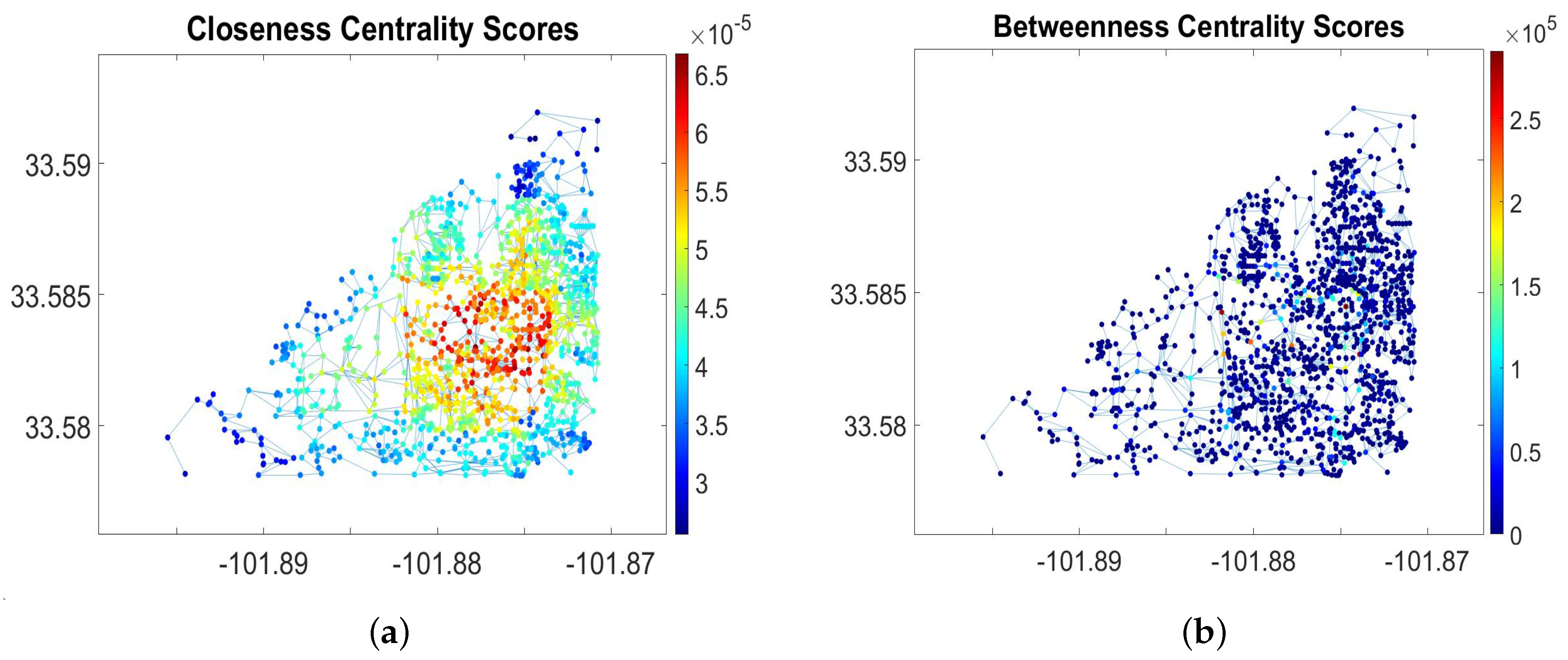In particular, the positive vector $u_1$, $u_{1,i}>0,$ known as the graph eigenvector centrality, is the major (Perron–Frobenius) eigenvector of the graph adjacency matrix A belonging to the maximal eigenvalue ${\alpha }_{\max }.$ The eigenvector centrality has been in use for more than a century [23] as the unique measure satisfying natural axioms for a ranking system [24]. A high eigenvector score means that a node hosts a relatively large share of infinitely long paths available in the graph being connected to many nodes who themselves have high scores.

We introduced thermodynamic (Gibbs [25]) ensembles of very long walks $n\to \infty$ in undirected connected graphs that elucidate the graph structure. These ensembles help to quantify accessibility, navigability, and the nodes’ strive in the graph, and evaluate the fugacity of graph nodes—the ease of their withdrawal from the graph—with respect to the entire system of available infinite walks [26]; this concept has been further studied [27,28]. In the following, we briefly discuss the statistical mechanics of very long walks in graphs and their applications for geometrization and navigability of the network, including the new results on transportation network geometrization under the conditions of traffic noise and fluctuating transportation capacity.

2.1. The Microcanonical Ensemble of Walks

The free energy of walks of length n (which we will call the n-walks) in the microcanonical ensemble of walks (MCE) equals $F_n={log}_2{\mathcal{N}}_n$, where ${\mathcal{N}}_n$ is the total number of n-walks available in the graph, G [26]. The free energy $F_n$ grows with n with the exponential rate—graph topological entropy (GTE) $\mu ={log}_2{\alpha }_{max},$ as $n\to \infty$. Irrelevant to the starting node of the walk, all MCE n-walks are assigned the same probability $P_n=exp\left(F_n/kT\right)$, where the (Boltzmann constant and) temperature $kT\equiv 1/ln2$. Therefore, GTE $\mu$ plays the role of a chemical potential for the system of infinitely long equiprobable walks available in the graph, G.

2.2. Entropic Pressure and Force Associated with the MCE Walks

Graph structural defects (missing nodes and edges) reshape the global mobility patterns in the graph, as they reduce the number (and trajectories) of many long walks, changing the free energy of walks dramatically. Indeed, by withdrawing a node $i\in V$ from the graph, we reduce the number of available MCE-walks ${\mathcal{N}}_n$ in that, and, consequently, the free energy of n-walks $F_n$ decreases by the following amount:

$${\left.\Delta \mathcal{F}\right|}_i=-\underset{n\to \infty }{lim}{log}_2\left(\frac{{\sum }_{ij}{\left(A^n\right)}_{ij}-{\sum }_j{\left(A^n\right)}_{ij}}{{\sum }_{ij}{\left(A^n\right)}_{ij}}\right)=-{log}_2\left(1-\frac{u_{1,i}}{{\gamma }_1}\right)\equiv \mathrm{Pressure}\left(i\right),{\gamma }_1\equiv \sum _{i=1}^N{u}_{1,i}$$

(1)

which we call entropic pressure [26], as quantifying the displacement of the walker’s mobility pattern from node $i\in V$ to other nodes of the graph if node i occasionally becomes unavailable. The components of the major eigenvector $u_{1,i}$ can be normalized as the eigenvector centrality scores, i.e., in such a way that ${\gamma }_1=1$, and then the expression in (1) takes an elegant form, viz., $\mathrm{Pressure}\left(i\right)=-{log}_2(1-u_{1,i})$, so that

$$\mathrm{Eigencentrality}\left(i\right)=1-2^{-\mathrm{Pressure}\left(i\right)}.$$

(2)

In the following, we assume that entries of $u_1$ are properly normalized and set ${\gamma }_1=1.$

Furthermore, by eliminating an edge $(i,j)\in E$ from the graph, we reduce the local free energy of the node i by an amount corresponding to the number of $(n-1)$-walks available from node $j\in V$ adjacent to i in the graph G, which takes the following form in the limit $n\to \infty$:

0

$$\mathrm{Force}(i,j)\equiv \underset{n\to \infty }{lim}-{log}_2\left(\frac{{\sum }_s{\left(A^n\right)}_{is}-A_{ij}{\sum }_k{\left(A^{n-1}\right)}_{ik}}{{\sum }_s{\left(A^n\right)}_{is}}\right)=-{log}_2\left(1-\frac{A_{ij}{u}_{1,j}}{{\alpha }_{max}{u}_{1,i}}\right)$$

(3)

which we call the entropic force [26] emerging from the statistical tendency of random walkers to prefer transitions to the nodes of higher eigenvector centrality scores (i.e., hosting more very long walks), than to those of lower centrality, despite their immediate connectivity (degree).

2.3. The Canonical Ensembles of Walks

In the framework of canonical ensembles (CNE), many particular long walks available in a graph (microstates) are lumped to one macrostate that can be characterized by a stationary distribution, or a density over graph nodes, their subsets, and walks [27]. The CNEs are formed by n-walks taken with equal probability, provided that they start at the same vertex i, $i\in V$ [26]. These (random) walks are described by the following irreducible row-stochastic transition matrices:

$$W_{ij}^{\left(n\right)}=\frac{A_{ij}{\kappa }_j^{\left(n\right)}}{{\kappa }_i^{\left(n+1\right)}},{\kappa }_i^{\left(n\right)}\equiv \sum _{j=1}^N{\left(A^n\right)}_{ij},{\kappa }_i^{\left(0\right)}=1,$$

(4)

in which ${\kappa }_i^{\left(n\right)}$ is the n-th order degree of vertex $i\in V$, in particular, ${\kappa }_i^{\left(1\right)}$ is the number of edges that are incident to vertex i in the graph. The random walk $W_{ij}^{\left(1\right)}=A_{ij}/{\kappa }_i^{\left(1\right)}$$\equiv A_{ij}/deg\left(i\right)$ is isotropic, as the corresponding transitions have no directional bias, and the next node to visit under such a walk is chosen equiprobably among all nearest neighbor nodes available in the graph. All ${\kappa }_i^{\left(n\right)}$ walks available from node $i\in V$ are chosen with equal probability by other random walks defined by $W_{ij}^{\left(n\right)}$, $n>1,$ so that immediate transitions may be directionally biased (anisotropic) toward the neighbor nodes, providing more lengthy paths than others [26]. The series $W_{ij}^{\left(n\right)}$ converges for infinite walks $n\to \infty$ to the Ruelle–Bowen random walk (RBW) [29], viz.,

$$W_{ij}^{\left(\infty \right)}=\underset{n\to \infty }{lim}{W}_{ij}^{\left(n\right)}=\frac{A_{ij}{u}_{1,j}}{{\alpha }_{max}{u}_{1,i}}=1-2^{-\mathrm{Force}(i,j)}$$

(5)

where $\mathrm{Force}(i,j)$ is the entropic force defined in (3). In the sections that follow, RBW denotes the anisotropic random walks. The CNE walks are characterized by equilibrium densities, the major left eigenvectors of the transition matrices $W_{ij}^{\left(n\right)}$ belonging to their maximal eigenvalue $\lambda =1$, viz.,

$${\pi }_i^{\left(n\right)}=\frac{{\kappa }_i^{\left(n\right)}{\kappa }_i^{\left(n-1\right)}}{{\sum }_{s=1}^N{\kappa }_s^{\left(n\right)}{\kappa }_s^{\left(n-1\right)}},\sum _{s=1}^N{\pi }_r^{\left(n\right)}{W}_{rs}^{\left(n\right)}={\pi }_s^{\left(n\right)}$$

(6)

that do not evolve over time. The equilibrium densities (6) are related to the node’s centrality measures. For example, ${\pi }_i^{\left(1\right)}={\kappa }_i^{\left(1\right)}/2\left|E\right|$ where $\left|E\right|$ is the graph edge number, corresponds to the degree centrality of a node. The stationary distribution for the RBW, ${\pi }_i^{\left(\infty \right)}=u_{1,i}^2$ [30], is the squared eigenvector centrality $u_{1,i}$ of node i [23,24].

The CNE walks defined in a finite-connected graph assign densities (i.e., probability distributions) to all graph nodes and nodal subsets of the graph with respect to a chosen diffusion process [28]. As a result, uncertainty about the admissible patterns of possible traffic in the network may be partially resolved (as characterized by some probability) [27], and navigability to a node may be assessed quantitatively with respect to the given graph structure. Moreover, as the probability distributions associated with the CNE walks generate a set of probabilistic metrics [31,32] similar to the resistance distance [33,34], we can quantitatively assess the isolation and integration of a node in the graph structure, as well.

2.4. Evaluating Structural Isolation and Integration by CNE Walks

The natural definition of the graph distance between two vertices in a graph, as the number of steps (graph’s edges) in the shortest path connecting them, can be generalized for random walks, provided that no loops are allowed—meaning the walkers do not revisit nodes they have already visited. Namely, the related distance may be defined as the expected commute time (CMT) between nodes by such a self-avoiding random walk [31,32]. Then, the accessibility to a node can be assessed by the expected first passage time (FPT) to the node by a self-avoiding random walk (from a node chosen at random over all nodes of the graph). While the node degree quantifies the local characteristic of a node, referred to as connectivity, the FPT quantifies the global connectedness of the node with respect to the entire graph structure, as it takes into account all possible paths to the node available in the graph, G, although some paths are more probable than others.

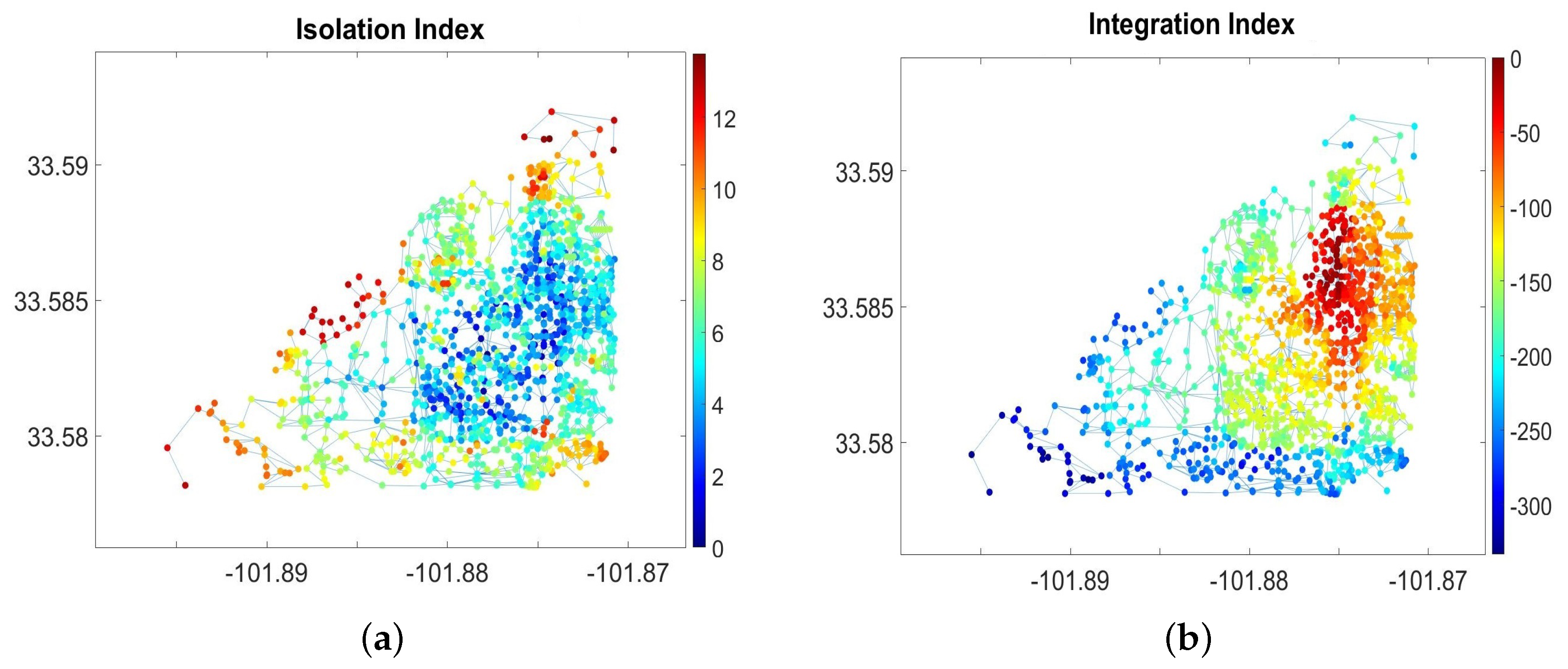
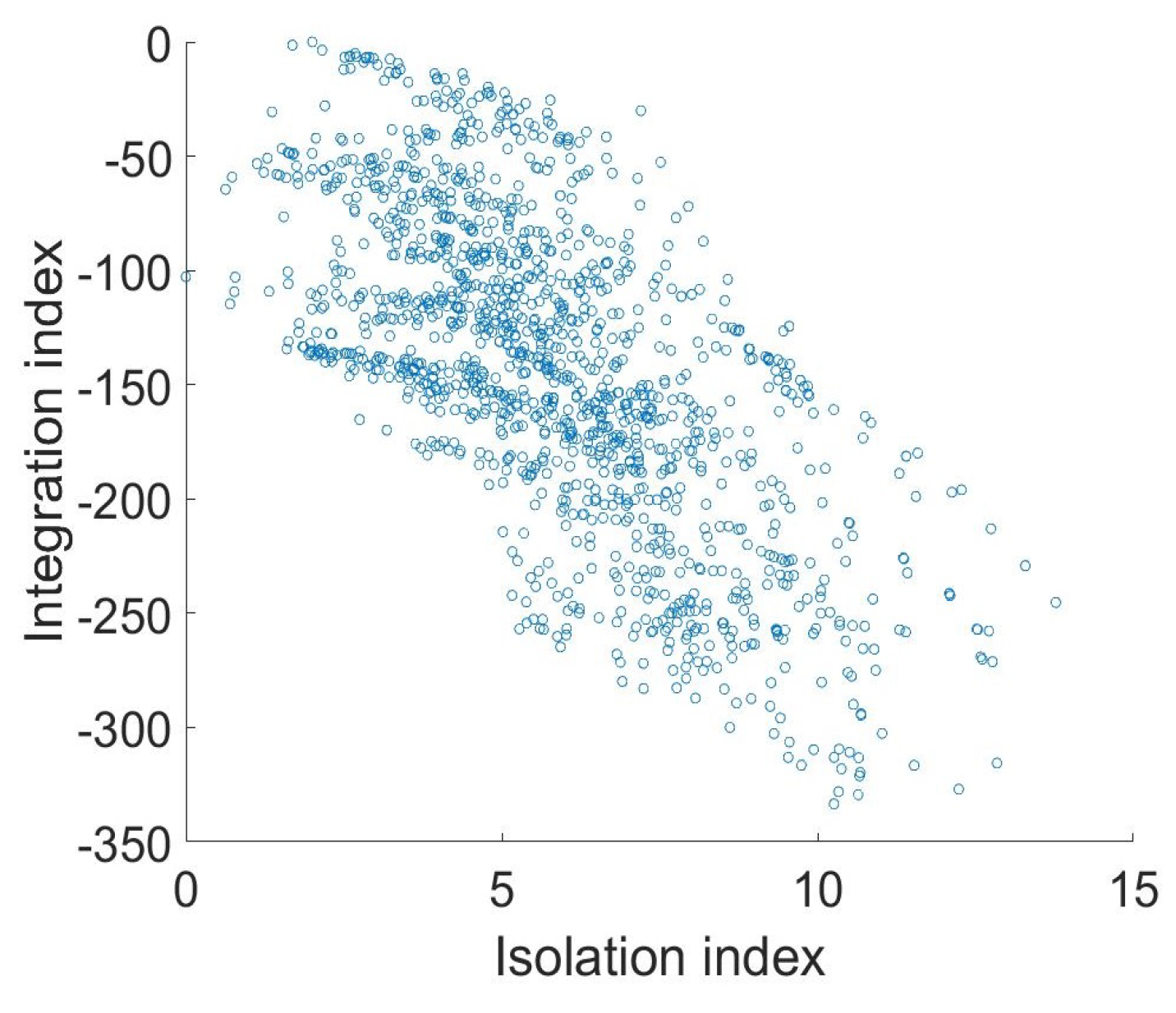
Isolation index of a node (ISL): In [35], we introduced the isolation index of a node (ISL), characterizing the node’s accessibility in the graph G as a relative FPT to the node measured in the decibel scale, viz.,

$$\mathrm{ISL}\left(i\right)=10·{log}_{10}\left(\frac{{\mathrm{FPT}}_1\left(i\right)}{{min}_{j\in V}{\mathrm{FPT}}_1\left(j\right)}\right)\left(dB\right),$$

(7)

in which ${\mathrm{FPT}}_1\left(i\right)$ is the FPT to the node required for a random walker following the isotropic random walk strategy defined by the transition matrix $W^{\left(1\right)}$. Isotropic random walks are insensitive to the structural heterogeneity, defects, and boundaries of a graph. This is because they take all available edges from a node equiprobably, thereby visiting all graph nodes according to their immediate connectivity (degree) [32]. The positive high values of the isolation index (7) are attributed to nodes that are relatively difficult to access in the graph (as measured by the isotropic FPT), and vice versa.

Integration index of a node (INT): The integration index of a node (INT) is defined as the inverse relative FPT—${\mathrm{FPT}}_{\infty }\left(i\right)$—to node $i\in V$ by the anisotropic RBW random walks $W_{ij}^{\left(\infty \right)}$ in the decibel scale [35], viz.,

$$\mathrm{INT}\left(i\right)=10·{log}_{10}\left(\frac{{min}_{j\in V}{\mathrm{FPT}}_{\infty }\left(j\right)}{{\mathrm{FPT}}_{\infty }\left(i\right)}\right)\left(dB\right).$$

(8)

Definition (8) is based on the intuition that areas and places of motion—morphemes—well-integrated into the urban fabric should belong to the majority of possible infinite walks existing in the graph and, therefore, determine the dominant mobility pattern in the transportation network. The RBWs are statistically inclined toward vertices that channel the majority of very long paths available in the graph, while avoiding graph defects and boundaries. According to definition (8), the node with the minimal FPT by RBWs has a zero score. Well-integrated vertices are characterized by near-zero values of the INT while the weakly integrated nodes have large negative scores.

The calculation of the FPT and the related first-attaining times are discussed in the forthcoming paragraphs.

FPT and Network Geometrization by the CNE Walks: The symmetrization transformation [27,32] modifies the Markov chain transition matrix $W_{ij}^{\left(n\right)}$, $n\ge 1,$ into a symmetric form, viz.,

$${\widehat{W}}_{ij}^{\left(n\right)}=\sqrt{\frac{{\kappa }_i^{\left(n\right)}}{{\kappa }_i^{(n+1)}}}{A}_{ij}\sqrt{\frac{{\kappa }_j^{\left(n\right)}}{{\kappa }_j^{(n+1)}}},{\kappa }_i^{\left(n\right)}\equiv \sum _{j=1}^N{\left(A^n\right)}_{ij},$$

(9)

and then the spectral theorem implies that $\widehat{W}$ is diagonalizable, viz., $\widehat{W}=\mathsf{\Phi }\mathsf{\Lambda }{\mathsf{\Phi }}^{\top }$ where $\mathsf{\Phi }\in O\left(N\right)$ is an orthogonal matrix of the orthonormal columns ${\varphi }_k:V\to S_1^{N-1}$, the eigenvectors of the transition matrix (9), and $\mathsf{\Lambda }$ is a diagonal matrix of real eigenvalues of the transition matrix that we consider to be ordered, viz., $1={\lambda }_1>{\lambda }_2\ge \dots \ge {\lambda }_N\ge -1$. To simplify the notation, we drop the index $\left(n\right)$ in the expressions of the present section, such as the symmetrized transition matrix (9).

The expected number of steps required for a self-avoiding (with no trajectory self-intersections) random walker started at node $i\in V$ to reach node j for the first time—the first-hitting-time (FHT)—satisfies the following matrix equation:

$$H_{ij}=1+\sum _{i\sim s}{H}_{sj}{W}_{si},H_{ii}=0.$$

(10)

The spectral representation of the solution of (10) [32,36] given by

$$H_{ij}=\sum _{s=2}^N\frac{1}{1-{\lambda }_s}\left(\frac{{\varphi }_{s,j}^2}{{\varphi }_{1,j}^2}-\frac{{\varphi }_{s,i}{\varphi }_{s,j}}{{\varphi }_{1,i}{\varphi }_{1,j}}\right)$$

(11)

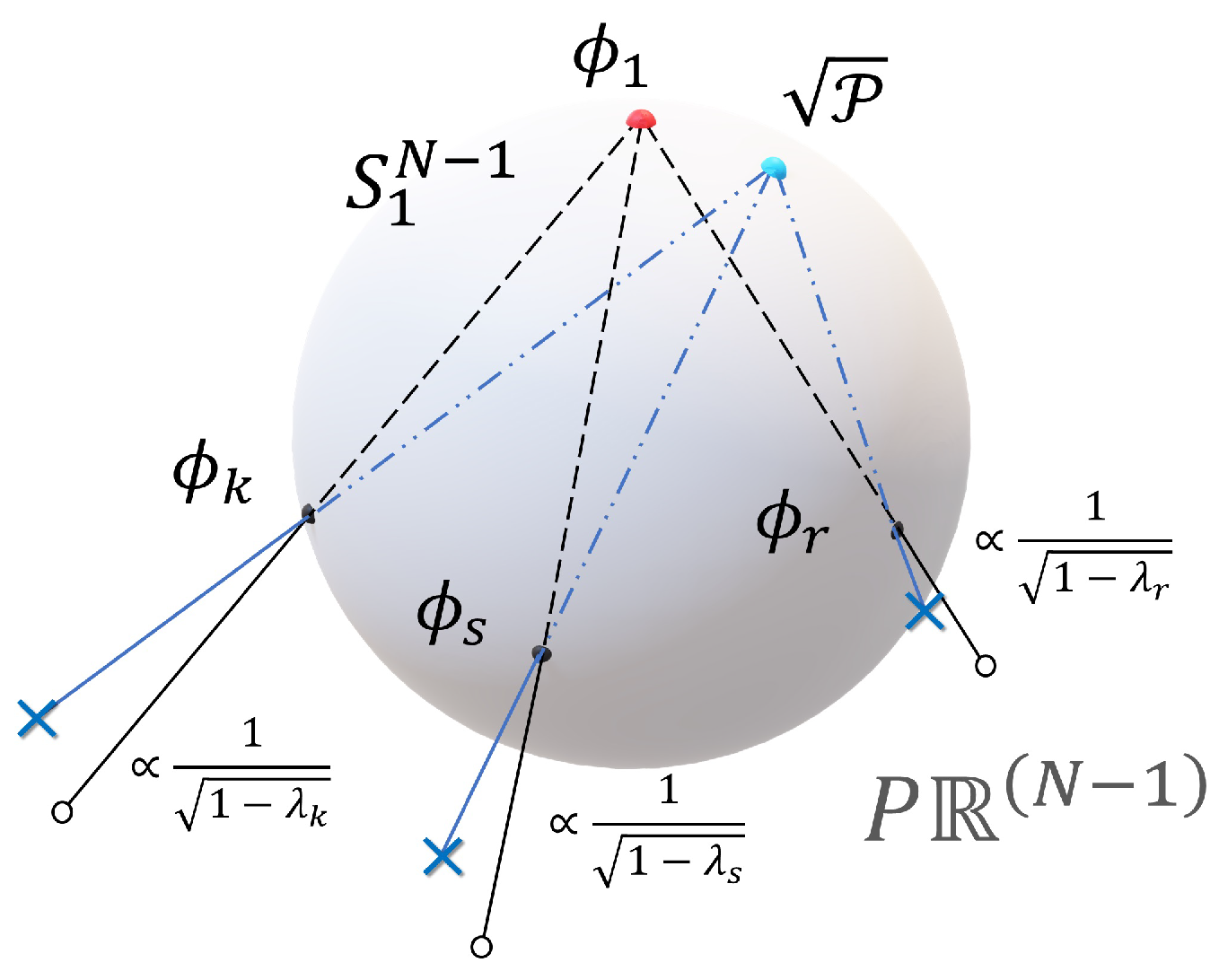
has the form of a stereographic projection onto projective $(N-1)$-dimensional space $P{\mathbb{R}}^{(N-1)}\left(V\right)$ where the stationary distribution of random walks $\left({\pi }_i={\varphi }_{1,i}^2\right)$ represented by the polar point ${\varphi }_1$ on the unit sphere (see Figure 1) is a projection point.

The global spectral characteristic of accessibility to a node in the graph is characterized by the random target access time (RTA), which is the expected length of a random walk with no loops, to reach a random target node, chosen with respect to the stationary distribution of walks $\pi$ [32,36], viz.,

$$\mathrm{RTA}\left(G\right)\equiv \sum _{j\in V}{H}_{ij}{\pi }_j=\sum _{j\in V}{H}_{ij}{\varphi }_{1,j}^2=\sum _{s=2}^N\frac{1}{1-{\lambda }_s}.$$

(12)

Then, the FPT is the expected length of a random walk with no loops allowed, to reach node $i\in V$ for the first time, starting from a random node, chosen with respect to the stationary distribution $\pi$, viz.,

$$\mathrm{FPT}\left(i\right)\equiv \sum _{j\in V}{\pi }_j{H}_{ji}=\sum _{j\in V}{\varphi }_{1,j}^2{H}_{ji}=\sum _{s=2}^N\frac{1}{1-{\lambda }_s}\frac{{\varphi }_{s,i}^2}{{\varphi }_{1,i}^2}.$$

(13)

According to (13), the FPT can be interpreted as a squared norm of the stereographic projection of the vector ${\varphi }_s\in S_1^{N-1}$, $s=2,\dots N$ from the polar point ${\varphi }_1$ on an $(N-1)$-dimensional unit sphere $S_1^{N-1}$ onto a projective space $P{\mathbb{R}}^{(N-1)}$ (see Figure 1) scaled by the factor $1/\sqrt{(1-{\lambda }_s)}$, and correspondingly, each graph node $i\in V$ is characterized by $(N-1)$ coordinates in $P{\mathbb{R}}^{(N-1)}$, viz., $\overrightarrow{i}={\left\{{\varphi }_{s,i}/{\varphi }_{1,i}\sqrt{(1-{\lambda }_s)}\right\}}_{s=2}^N$.

Finally, the CMT time, i.e., the expected length of a commuting walk between i and j with no loops allowed, plays the role of a (Euclidean) distance in the projective space $P{\mathbb{R}}^{(N-1)}$ [32,36], viz.,

$$\mathrm{CMT}(i,j)\equiv H_{ij}+H_{ji}=\sum _{s=2}^N\frac{1}{1-{\lambda }_s}{\left(\frac{{\varphi }_{s,i}}{{\varphi }_{1,i}}-\frac{{\varphi }_{s,j}}{{\varphi }_{1,j}}\right)}^2.$$

(14)

The average of CMT (14) over the starting nodes of a walk equals the sum of the FPT to node j from a random node (13) and the RTA (12) from j to a random node, viz., ${\sum }_i{\pi }_i\mathrm{CMT}(i,j)=\mathrm{RTA}\left(G\right)+\mathrm{FPT}\left(j\right)$. Finally, the double average of CMT (14) equals the doubled RTA, viz., ${\sum }_{i,j}{\pi }_i\mathrm{CMT}(i,j){\pi }_j=2\mathrm{RTA}\left(G\right).$ We can conclude from (13) and (14) that random walks equip a connected undirected graph with the Euclidean metric associated with the first-attaining times to the nodes in the corresponding graph structure.

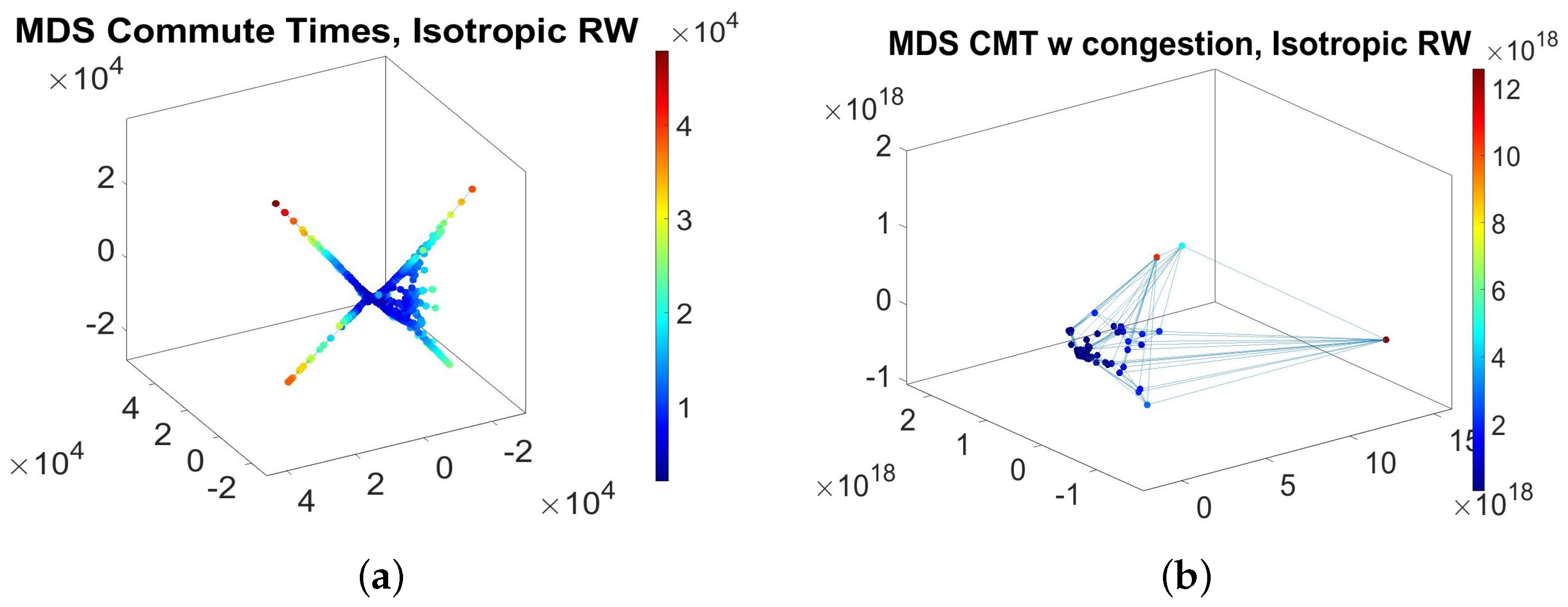
The (Euclidean) CMT distances between N-graph vertices (14) can be visualized with the use of the multidimensional scaling method (MDS) metric, a form of non-linear dimensionality reduction mapping the nodes into a configuration of N points in an abstract lower-dimensional Cartesian space [37,38] that minimizes a residual sum of squares, viz.,

$$\sqrt{\sum _{i\ne j=1,\dots ,N}{\left(CMT(i,j)-\parallel x_i-x_j\parallel \right)}^2}.$$

(15)

The MDS technique may be used to place the graph nodes into a two- or three-dimensional Euclidean space, such that the distances between nodes are as close to the values $CMT(i,j)$ as possible, visualizing the level of similarity in the accessibility traits in the spatial graph.

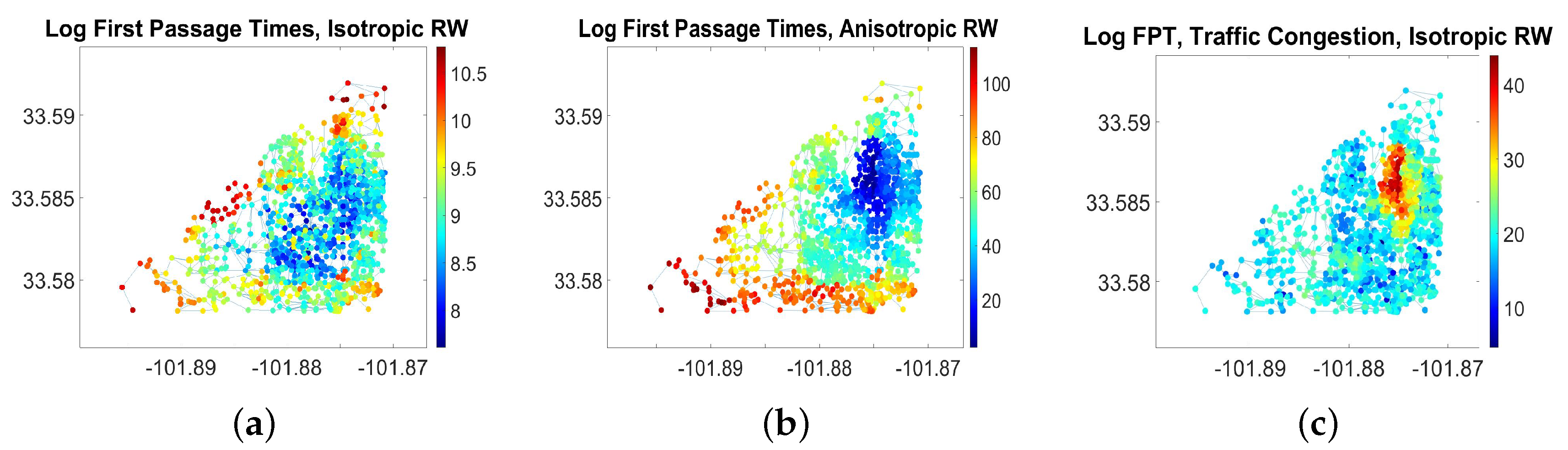
Indeed, the geometric quantities (13) and (14) defined above depend dramatically on the chosen random walk strategy determined by the particular Markov chain transition matrix $W_{ij}^{\left(n\right)}$, $n\ge 1$. In our paper, we denote the FPT (13) to a node calculated with respect to the isotropic random walks $W_{ij}^{\left(1\right)}$ as ${\mathrm{FPT}}_1\left(i\right)$. In our approach, we use this quantity to assess isolation, the $\mathrm{ISL}\left(i\right)$ of a node (7). To evaluate integration, the $\mathrm{INT}\left(i\right)$ of a node (8), we use the FPT (13) calculated for the anisotropic RBW random walks (5) and denoted as ${\mathrm{FPT}}_{\infty }\left(i\right)$. As the RBW walks (5) are statistically bound to the graph nodes hosting the majority of very long walks, but repelled from the graph structural defects and boundaries, ${\mathrm{FPT}}_{\infty }\left(i\right)\ll {\mathrm{FPT}}_1\left(i\right)$, for the walking hubs i, at the crossroads of very long walks, far apart from the graph structural irregularities, even though their immediate connectivity (degree) is not very high. Alternatively, considering that the probability of finding an RBW-walker in a remote node $i\in V$, which is not significant for the system of very long walks in the graph, is very low, we can conclude that for such a node, it should be ${\mathrm{FPT}}_{\infty }\left(i\right)\gg {\mathrm{FPT}}_1\left(i\right)$.

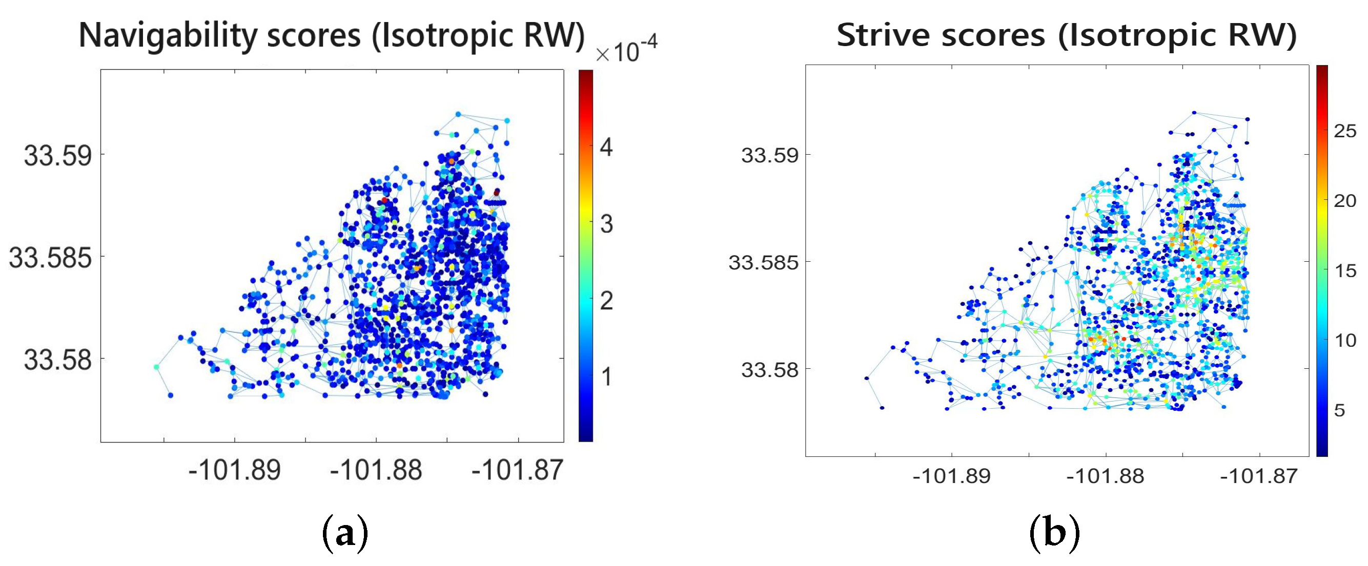
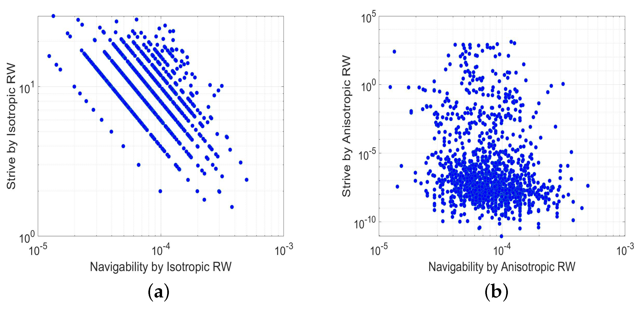
2.5. Assessing Navigability and Strive by the CNE Walks

The more frequent a node, the more predictable the navigator’s location in it [26,39]. The CNE walks assigning densities to all nodes (6) and nodal subsets in the graph allow for quantifying navigability for graph nodes [26,27,35]. Indeed, the amount of information resolving uncertainty at each step of infinitely long sequences $\left\{X_t\right\}$, $t\ge 0,$ of a Markov chain defined by a transition matrix W between a finite set of N states equals the Boltzmann–Gibbs–Shannon entropy [27,35,40,41],

$$\mathfrak{H}\left(X_t\right)=-\sum _{i=1}^N{\pi }_i{log}_N{\pi }_k,$$

(16)

in which $\pi$ is a density of states ${\{i\in V\}}_{i=1}^N$ in the Markov chain, and we assume that $0·log0=log{0}^0=log1=0$, as usual. The amount of uncertainty (16) can be represented as a sum of the predictable information component, $\mathfrak{P}\left(X_t\right)\equiv -{\sum }_{i=1}^N{\pi }_i·{log}_2{\phi }_i,$ measuring the amount of apparent uncertainty about the navigator’s location, and the unpredictable information component $\mathfrak{U}\left(X_t\right)\equiv -{\sum }_{i=1}^N{\pi }_i·{log}_2{\psi }_i$ that assesses the amount of true uncertainty about the walker’s current position, [26,28,42], viz.,

$$\mathfrak{H}\left(X_t\right)=\mathfrak{P}\left(X_t\right)+\mathfrak{U}\left(X_t\right)=-\sum _{i=1}^N{\pi }_i·{log}_2{\phi }_i-\sum _{i=1}^N{\pi }_i·{log}_2{\psi }_i,{\pi }_i\equiv {\phi }_i{\psi }_i.$$

(17)

The partition functions ${\phi }_i$ and ${\psi }_i$, quantifying the amounts of predictable and unpredictable information about the navigator’s location, can be called the navigability and strive potentials of node $i\in V$, respectively [28], viz.,

$${\phi }_i\equiv {\pi }_i·\prod _{j=1}^N{\left(W_{ij}^2\right)}^{W_{ij}^2},{\psi }_i\equiv \prod _{j=1}^N{\left(W_{ij}^2\right)}^{-W_{ij}^2}.$$

(18)

The amounts of predictable and unpredictable information (18) vary over the Markov chain and, for CNE walks defined on a graph, depend on the chosen random walk strategy $W^{\left(n\right)}$, as well as the relative importance of a node for the walks [28]. It is also worth mentioning that the product ${\prod }_{j=1}^N{\left(W_{ij}^2\right)}^{W_{ij}^2}$ in (18) is nothing else but a geometric mean of 2-step transition probabilities between i and j representing the time averages over an infinitely long Markov chain. Therefore, the navigability potential ${\phi }_i$ quantifies a chance that node i may be a precursor to another node that may occur in the walk two steps after i. Consequently, the inverse probability ${\prod }_{j=1}^N{\left(W_{ij}^2\right)}^{-W_{ij}^2}$ in the above definition of strive potential equals the expected time required for a two-step neighborhood exploration of node i, the neighborhood exploration time. The more extensive the node’s neighborhood, the longer the time required for exploration, the stronger the strive potential of the node, reducing navigability, i.e., the amount of predictable information about the location of random walkers [28].

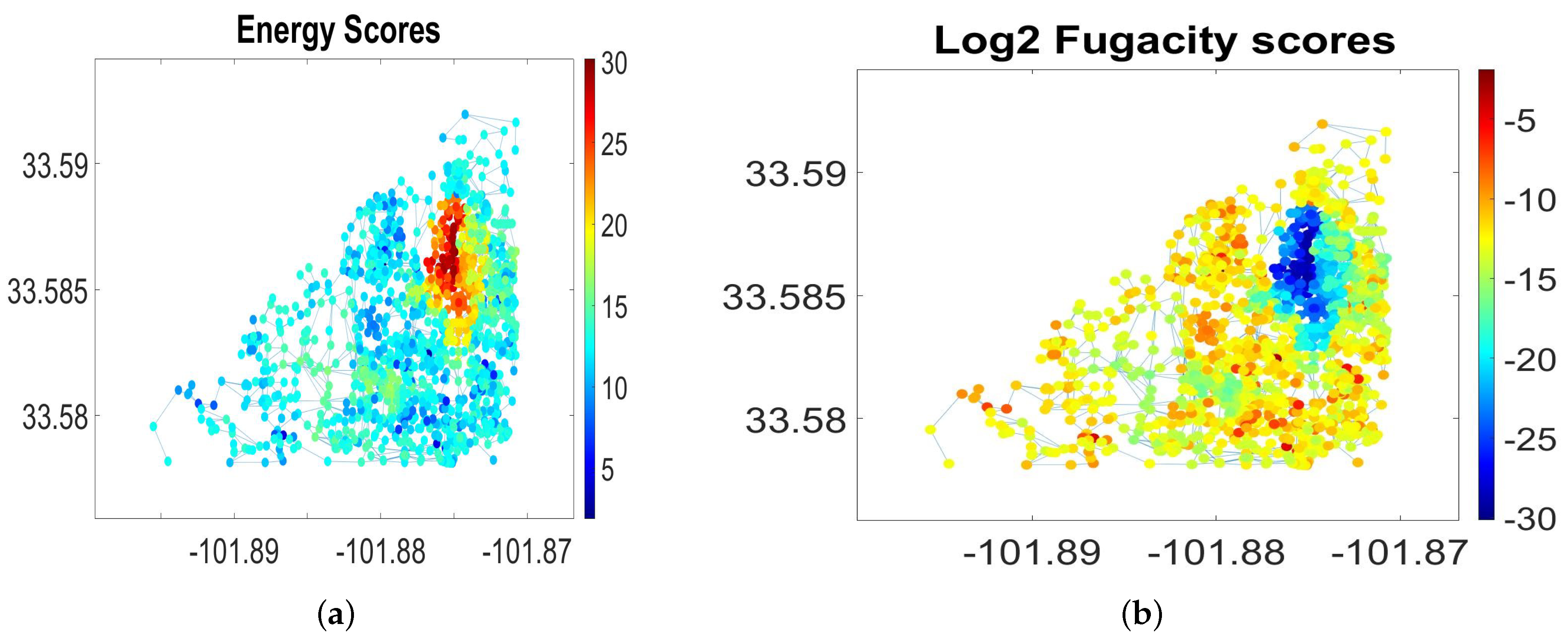
2.6. The Grand Canonical Ensemble of Walks

The grand canonical ensemble (GCE) of walks describes the statistics of fluctuations of the local growth rate ${log}_2{\kappa }_i^{\left(n\right)}$ of the number of distinguishable n-walks available from a node around the global growth rate, $n\mu ={log}_2\left({\alpha }_{max}^n\right)$, predicted by the GTE $\mu ,$ playing the role of a “chemical potential” for the entire system of infinitely long equiprobable walks [26,27,28]. The graph is considered open to modifications, similar to a thermodynamic system exchanging energy and particles with a heat bath in thermodynamic equilibrium, as described by Gibbs [25]. In the thermodynamic limit of infinite walks, $n\to \infty$, the Gibbs-type exponential factor, known as node’s fugacity, describing the ease of withdrawing a node from the graph considered to be in a thermodynamic equilibrium with the environment [27], takes the following form:

$$\mathrm{Fugacity}\left(i\right)\equiv \underset{N\to \infty }{lim}exp\left(\frac{n\mu -{log}_2{\kappa }_i^{\left(n\right)}}{kT}\right)=\frac{1}{u_{1,i}}.$$

(19)

where we assume that the major eigenvector $u_1$ is properly normalized, i.e., ${\sum }_{j=1}^N{u}_{1,j}=1$. According to the definition given above, the value of the fugacity parameter is nothing else but the inverse eigenvector centrality, and, therefore, its value is small for the high eigenvector centrality nodes, hosting the majority of infinitely long paths available in the graph, and vice versa (the nodes of high fugacity (low centrality) can easily be withdrawn from the graph).

The GCE probability (to observe a local fluctuation of fugacity at $i\in V$ for the infinite walks, $n\to \infty$) takes the form of a Fermi–Dirac distribution (FDD), which is typical for non-interacting fermions in a single-particle state i, viz.,

$${\mathcal{P}}_i=\frac{u_{1,i}^{-1}}{{\sum }_{j\ne i}^N{u}_{1,j}^{-1}}\equiv \frac{1}{1+exp\left(\frac{{\mathcal{E}}_i-\mathfrak{M}}{kT}\right)}$$

(20)

where $\mathfrak{M}=0$ is a zero chemical potential, the specific energy that can be absorbed or released in our model due to removing or adding a node from or to the graph, provided it does not affect the entire system of infinite walks in it. The temperature is defined as $kT\equiv 1/ln2$, and the energy ${\mathcal{E}}_i$ of the i-th state, viz.,

$${\mathcal{E}}_i={log}_2\left(u_{1,i}\sum _{j\ne i}^N\frac{1}{u_{1,j}}\right)\equiv \mathsf{\Omega }+{log}_2\left(u_{1,i}\right),\mathsf{\Omega }\equiv {log}_2\left(\sum _{j=1}^N\frac{1}{u_{1,j}}\right),$$

(21)

in which $\mathsf{\Omega }$ is the grand canonical potential of the entire system of infinite walks possible in the graph. The GCE probability distribution (20) quantifies the chances of node $i\in V$ being withdrawn from the graph in proportion to the impact that such a withdrawal would have on the entire system of infinitely long walks. The vertices with the inferior growth rate of the number of very long walks available from them are considered as being loosely integrated into the graph structure; therefore, they might be easily removed from the graph, or, on the contrary, acquire some new connections during the course of graph structural modifications. It is worth mentioning that, as infinite walks in a graph do not interact with each other, our model is statistically similar to a quantum system subjected to the Pauli exclusion principle, which causes the FDD to appear in (20). Moreover, the FDD for a node’s fugacity also appears as the unique stationary solution for a Fokker–Planck equation describing the continuous-time dynamics of transport under the conditions of traffic noise and fluctuating transportation capacity of graph edges, or a random edge rewiring in a transportation graph when centrality flips its role in the network dynamics [27,43,44]. Indeed, the traffic congestion and consequent accumulation of walkers in a “noisy” transportation network would occur at the nodes of lowest centrality and in structural bottlenecks rather than in hubs handling the majority of traffic under the normal operation regime in the network [27].

2.7. Transportation Network Geometry Distortion under the Conditions of Traffic Noise and Fluctuating Transportation Capacity

The equilibrium density of CNE walks emerging naturally under the condition of fluid traffic through the network has no meaning if the walkers become stuck in a random traffic jam or experience the occasional traffic slowdown caused by temporary traffic flow disruptions. In the latter case, in the analysis of first-attaining times given in Section 2.4, we replace the stationary distributions $\pi$ of random walks (6) with the GCE-distribution $\mathcal{P}$ of the node’s fugacity, defined by (20). In projective geometry of first-attaining quantities illustrated by Figure 1, this would correspond to the change in the projection point ${\varphi }_1$ by the point denoted as $\sqrt{\mathcal{P}}$, which is located in the same positive segment of the unit sphere as ${\varphi }_1$. The corresponding formulas for the first-attaining quantities under the conditions of random traffic flow disruptions are derived from (13) and (14), by the following replacement: ${\varphi }_{1,i}\to \sqrt{P_i}$, viz.,

$$\widetilde{\mathrm{FPT}}\left(i\right)=\sum _{s=2}^N\frac{1}{1-{\lambda }_s}\frac{{\varphi }_{s,i}^2}{{\mathcal{P}}_i}=\sum _{s=2}^N\frac{2^{\mathsf{\Omega }}}{1-{\lambda }_s}{\varphi }_{s,i}^2{u}_{1,i}$$

(22)

and

$$\widetilde{\mathrm{CMT}}(i,j)=\sum _{s=2}^N\frac{1}{1-{\lambda }_s}{\left(\frac{{\varphi }_{s,i}}{\sqrt{{\mathcal{P}}_i}}-\frac{{\varphi }_{s,j}}{\sqrt{{\mathcal{P}}_j}}\right)}^2=\sum _{s=2}^N\frac{2^{\mathsf{\Omega }}}{1-{\lambda }_s}{\left({\varphi }_{s,i}\sqrt{u_{1,i}}-{\varphi }_{s,j}\sqrt{u_{1,j}}\right)}^2$$

(23)

where $u_{1,i}>0$ are the eigenvector centrality scores of the graph nodes and $\mathsf{\Omega }$ is the grand canonical potential of infinite walks available in the graph. It is worth mentioning that, under the conditions of traffic noise and fluctuating transportation capacity, the first-attaining times (22) and (23) defined above may differ significantly from the quantities defined by (13) and (14).

3. Scene: Isolation, Integration, Segregation, and the Role of TTU Campus in the City of Lubbock

After the first train steamed to Lubbock on 25 September 1909, its population raised to 4000 in a 10-year period [45]. Establishing a public research university in Lubbock on 10 February 1923 (under the name of Texas Technological College) with just six buildings and an enrollment of 914 students on 1 October 1925 was another important milestone in the urban development, as the county population had grown rapidly to almost 40,000 by 1930. When the Belt Road Loop 289 encircled the town by the mid-1960s, Lubbock eventually turned into a city (Figure 2a). After nightfall on 11 May 1970, portions of Lubbock were struck by a powerful multiple-vortex tornado, resulting in 26 fatalities and damaging nearly 9000 homes and inflicting widespread damage to businesses, high-rise buildings, and public infrastructure [46]. The primary tornado touched down in southwestern Lubbock and carved an 8.5-mile (13.7 km) path of devastation, encompassing roughly a quarter of the city, with the most destructive impacts were observed in the northeastern part of the city, such as in the Guadalupe barrio, north of 4th Street, along Texas State Highway Loop 289, and near the Lubbock County Club where homes were completely leveled [47].

Although the tornado reshaped the city’s history, it caused relatively light damage to the campus of Texas Tech University. With its size of 1839 acres, the TTU campus, the second largest contiguous campus in the United States [48], settled at the city heart, provides the longest pedestrian walkways in Lubbock.

Although the railroad enhanced the city’s status in the early days, it cut the streets, fostering isolation in the nearby areas by dramatically reducing the number of available paths connecting the urban neighborhoods that were located on the opposite sides of the railway tracks. The extensive voids that remained in the northern and eastern parts of Lubbock, following the destructive impact of a tornado, were cut off from the rest of the core city by rails and were not restored for a quite long time. As a result, the city core was literally squeezed out from a bend carved by railways and thrust to the southwest, away from Loop 289 bounding the city before the mid-1960s (Figure 2a) [35]. Defects in connectivity can significantly decrease the number of infinite walks in a city graph, thereby altering the global mobility patterns that can be explained through entropic force. The statistical propensity of very long walks in the graph to preferentially transition to nodes with high eigenvector centrality, hosting numerous infinitely long walks, gives rise to a direction-dependent entropic force [26].

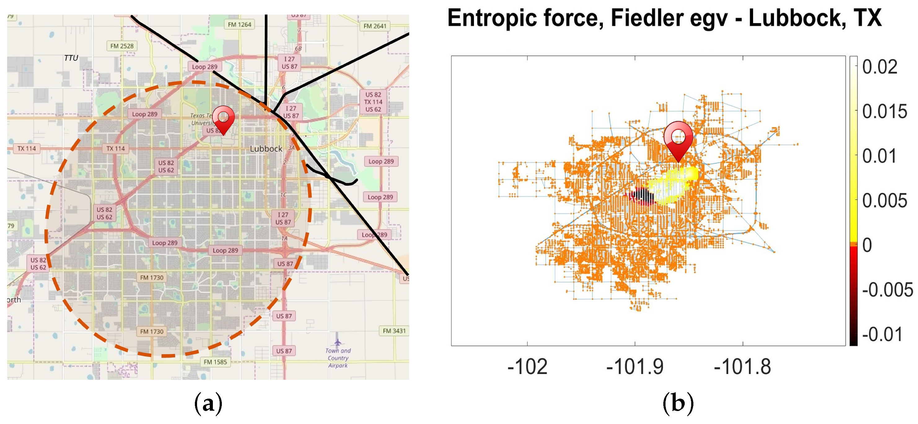
We utilized the graph representation of Lubbock, TX, obtained from the OpenStreetMap service [49] to depict the entropic force occurring in the spatial structure of TTU’s home city. The spatial graph adjacency matrix of Lubbock was constructed using Python’s lxml library by parsing the raw data and removing structurally disconnected neighborhoods. Lubbock’s linked city graph comprises 10,421 nodes, representing all modes of transportation, including but not limited to residential, secondary, and tertiary roadways, trunk linkages, and highways.

The city’s spatial network of Lubbock is shown in Figure 2b. The nodes acquired from the OpenStreetMap service are highlighted according to their scores in Fiedler’s eigenvector (used for the spectral bisection of graphs) belonging to the second largest eigenvalue of the $\mathrm{Force}(i,j)$-matrix defined in (3). The Fiedler eigenvector indicates the direction of the steepest descent of the entropic force $\mathrm{Force}(i,j)$ across the Lubbock city spatial graph. In exception for a thin zone anchored at the defunct city train station that extends from the historical city center (expelling infinite walks southwest), the entries of Fielder’s eigenvector are zero everywhere (Figure 2b) [26]. Needless to say, the TTU cannot follow Lubbock in expanding away from the old city boundaries, as it remains loyal to the former city center with its campus (Figure 2a). Situated on the boundary of the neighborhoods going downhill (Figure 2b), the University campus, being a hub for everyday college activities, serves as a bridge between the city of Lubbock’s patterns of isolation and integration (see Figure 3) [35].

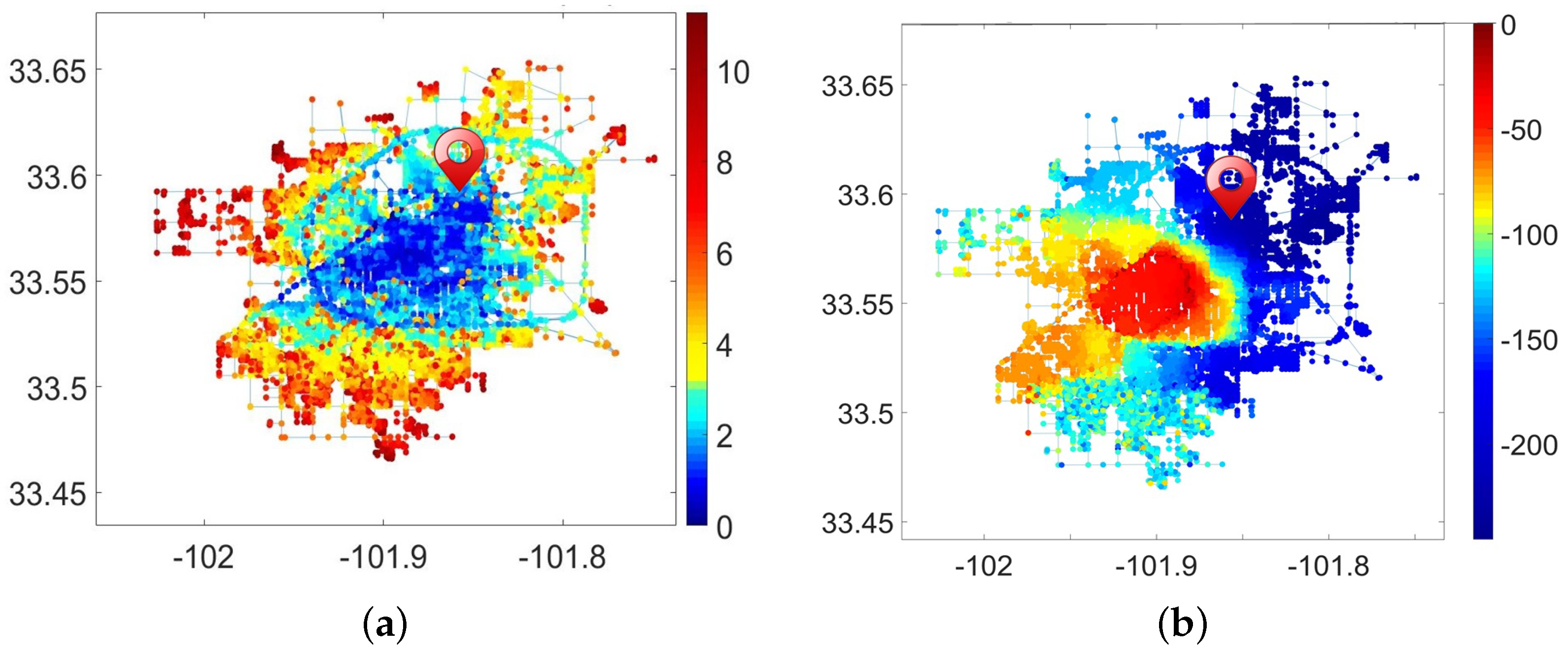
The isolation and integration patterns, as defined in (7) and (8) for the city of Lubbock, acquired from the OpenStreetMap service [49] (see Figure 3), are featured by the shortest FPT values with respect to the isotropic and anisotropic random walks. The high values of the isolation index (7) (red color in Figure 3a) are attributed to sprawling urban areas, homing the low-density communities, and auto-dependent urban developments laying outside the Belt Road, apart from the structural focus of the city. Interestingly, statistically defined integration and isolation patterns (8) and (7) do not always oppose each other, as some quiet places in sprawling areas of the wealthy southwestern part of Lubbock are relatively isolated, yet well-integrated into the system of very long paths possible in Lubbock’s spatial graph (Figure 3b).

The integration index of a place defined by (8) highlights a relative share of very long paths hosted by the place in the city street map. Places hosting the lion’s share of very long walks feature global mobility patterns in urban structures, playing the role of natural social and economic hubs of the city. Although located within the historic city borders, areas such as those in the northeastern portion of the city that are shut off from the center by commercial trains, significantly reducing the number of infinitely long pathways, are only sporadically incorporated into the city fabric. They are characterized by the large negative numbers of integration indexes (8) and colored in dark blue in Figure 3b. Due to the structural imbalance fostered by railways, relatively isolated sprawling areas of the southwest are able to statistically accumulate the bulk of possible infinite routes and move Lubbock’s mobility patterns from the historic core to the southwest suburbs; integrated isolation is not an oxymoron, but the home of the wealthiest people. The northeastern portions of Lubbock, cut off by railways and characterized by very low values of the integration index (dark blue in Figure 3b), align with the historical segregation patterns of spatial and land division, as well as ownership, early in the 20th century. This was when black workers and braceros (Mexican workers), as well as their families, settled in labor camps, in what is known today as Guadalupe Park and the surrounding areas. Numerous buildings throughout Lubbock were damaged beyond repair and were demolished after the tornado of 1970, including the northwestern section of downtown and the predominantly Hispanic neighborhood of Guadalupe in the northeast [50]. The Lubbock Urban Renewal Agency rebuilt the largely destroyed Guadalupe neighborhood, although progress was slow for many years before substantial reconstruction occurred [46,47,50]. Today, most of the Hispanic–Latino descent communities are still located in the northeast, living under the most pressuring social and economic issues [51].

4. Campus: Walkable Area Identification and Adjacency Matrix Generation

The original TTU campus layout and architecture of 1925 reflected the Spanish Renaissance Revival style. The campus continued to expand during the 1930s, with the addition of new academic and administrative buildings, such as the iconic Engineering Key and the Administration Buildings. The campus development slowed down during World War II due to budget constraints, but resumed after the war, and flourished in the 1950s and 1960s when new academic buildings, dormitories, and sports facilities were constructed. The university’s growth was accompanied by a shift in architectural styles, moving away from the Spanish Renaissance Revival to more modern designs. From the 1970s to 1990s, the campus development continued to reflect a blend of modern architecture and a commitment to preserving historical buildings. In the last decades, the campus underwent major transformations, with new state-of-the-art academic buildings, research centers, and student housing complexes, and presently continues to evolve with a focus on sustainability, technology, and innovation. Ongoing projects include the construction of modern research facilities, improvements to student amenities, and the integration of green spaces and outdoor areas for the campus community.

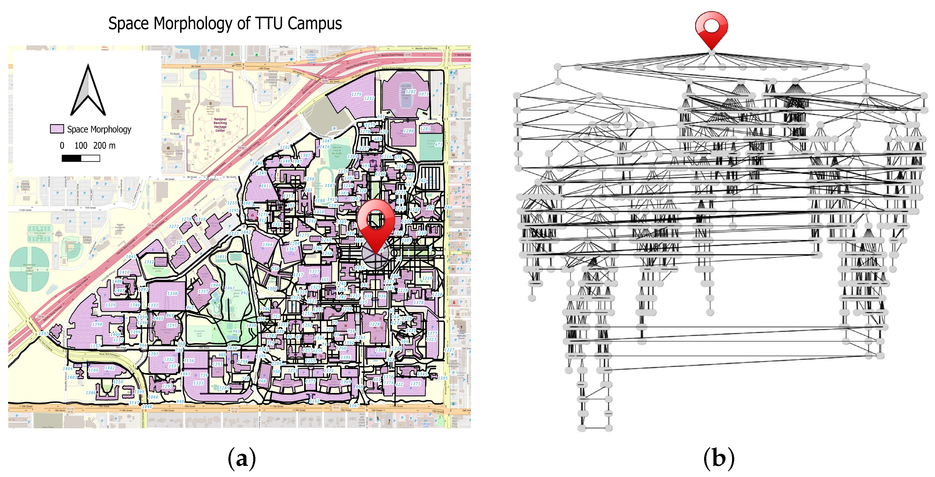
To assess the spatial morphology of the campus and its implications for pedestrian accessibility, the walkable spaces across the campus were identified through the utilization of QGIS. These areas encompassed various pedestrian pathways, including sidewalks and the footprints of buildings (see Figure 4a). By meticulously defining these walking spaces, we aimed to capture the spatial context of pedestrian movement within the campus environment. One innovative aspect of our methodology was the inclusion of buildings within the defined walkable areas. Recognizing that buildings often serve as connective elements within the campus, we delineated pathways that incorporated building structures. This acknowledgment was rooted in the understanding that certain buildings facilitate movement between different parts of the campus.

Each identified walking space was assigned a distinct identifier, resulting in the manual delineation of 1466 individual features or shape files within the QGIS software(3.34.1). These walkable zones were subsequently interconnected, reflecting the interplay between pedestrian paths and building structures. A pivotal step in our methodology involved conducting an intersection analysis between the designated walking spaces and the openings of buildings. This analysis was imperative as it directly influenced the accessibility and navigational feasibility of the pedestrian routes. By executing the intersection operation, we aimed to uncover critical points of interaction within the campus layout.

Following the intersection analysis, an adjacency matrix was generated. This matrix facilitated the visualization of relationships between different shape features identified in the walkable zones. Each row and column of the matrix represented a distinct shape feature, and the matrix elements denoted the presence or absence of intersections. Since pedestrian traffic in each area is possible in both directions, the spatial graph representing the campus morphology is undirected. In Figure 4b, we show a tree representation of the obtained spatial graph rooted at Memorial Circle, the most connected place on the TTU campus. Although the spatial graph structure of the TTU campus is ample with cycles (and, therefore, is not a tree, formally speaking), its tree representation shown in Figure 4b exhibits the profound depth of the spatial morphology (up to 26 levels) and the structural heterogeneity of the graph, revealing itself in the presence of many connected clusters, as well as the multiple structural bottlenecks.

5. Results: Morphology of the TTU Campus Pedestrian Network

The campus plays a pivotal role in the college experiences of students by providing various facilities and hosting diverse activities. The campus structure design plays a critical role in promoting or hindering regular walking and affects spatial accessibility to the different buildings and places of movement in the campus environment.

5.1. Functional Blindness of Shortest Paths Morphology

Some places in the CPN TTU are more “important” than others, shaping the possible movement patterns based on the shortest paths between nodes available in the graph. Here, the importance of a node may either be conceived in relation to a possible transfer process across the network, or as its involvement in the global cohesiveness of the CPN. In the first case, the distribution of centrality scores over the graph nodes is diffuse, with the highest centrality values for the nodes located at the graph core and the lowest values on the periphery. In Figure 5a, we present the spatial graph of TTU CPN with nodes, highlighting their closeness centrality scores, calculated as the reciprocal of the average length of the shortest paths between the node and all other nodes in the graph [52], viz.,

$$C\left(i\right)=\frac{N-1}{{\sum }_{j}d(i,j)}$$

(24)

where $d(i,j)$ is the distance (length of the shortest path) between vertices i and j in the spatial graph of TTU CPN. The graph shown in Figure 5a displays the closeness centrality core characterized by the highest scores (24) at the geographical and historical centers of the network.

Other centrality measures, such as betweenness centrality shown in Figure 5b, focus on the particular graph nodes that are pivotal to the global network’s connectedness, such as bridges and other structural bottlenecks. The betweenness centrality of a vertex i is a measure of the proportion of the shortest paths through the graph that passes through i [53], viz.,

$$B\left(i\right)=\frac{1}{N(N-1)}\sum _{j\ne i\ne k}\frac{{\sigma }_{jk}\left(i\right)}{{\sigma }_{jk}}$$

(25)

where ${\sigma }_{jk}$ is the total number of shortest paths from node j to node k and ${\sigma }_{jk}\left(i\right)$ is the number of paths that passes through i. Vertices of high betweenness have the potential to disconnect the pedestrian connection based on the shortest paths in the CPN graph if removed. These vertices are sparsely dispersed over the entire CPN, as shown in Figure 5b, indicating the presence of multiple structural bottlenecks in the network. In general, shortest-path morphology does not predict pedestrian behavior on campus and is unable to describe possible changes in this behavior in the case of campus structural modifications.

5.2. Campus Morphology —An Interplay between the Core and Periphery

Actual pedestrian walks across the CPN are far from those following the shortest paths available in the spatial graph. We would rather choose a route that will be pleasant and safe to walk than take the shortest cut to reach the destination in the shortest amount of time. Pedestrian pathways follow vehicle-free walkways in pedestrian-friendly environments that adhere to established norms, ensuring the overall efficiency and functionality of the campus [21]. Playing a vital role in facilitating student mobility within a campus environment, they serve as essential connectors, linking parking lots, bus stops, lecture halls, libraries, offices, and other key destinations. Campus walkability is influenced by both the constructed environment and the varying perceptions of students.

First-attaining times in the TTU CPN: The expected length of a random walk without loops needed to move from a randomly selected node to the node in question—FPT (13)—defines a Euclidean space metric (14) on any finite-connected undirected graph, with respect to the chosen random walk strategy [32]. The FPT scores can be used as a natural measure of the node’s accessibility compatible with our everyday (Euclidean) intuition and, therefore, they can be related to the human perception of urban space, governing our navigation and way-finding [54].

In Figure 6a, we show the distribution of the (logarithm) FPT values (13) over the nodes of the TTU CPN spatial graph by the isotropic random walks $W^{\left(1\right)}$ in Figure 6a and by the anisotropic random walks $W^{(\infty )}$ in Figure 6b. Isotropic random walks homogeneously cover all available spaces of motion, as being sensitive to their immediate connectivity rather than to the possible structural defects and area boundaries. On the contrary, anisotropic random walks are essentially sensitive to structural irregularities dwelling at the most integrated parts of graphs and central open spaces of the environment. The distribution of FPT values demonstrates a diffusive character in a sense that vertices located at the central part of the CPN’s spatial graph are characterized by relatively low FPT values while the nodes located at the graph periphery are more difficult to access and, therefore, can be perceived as being disconnected from the graph’s core.

The graph core of the TTU CPN coincides with the historical Texas Tech College layout established during the 1930s, marked by the relatively short FPT by anisotropic random walks, as clearly visible in Figure 6b. Indeed, studying the urban structure using the random walk method often allows one to understand its historical development. For example, FPT by (isotropic) random walks allows for identifying the historical locations of ghettos in Venice and New York [54,55]. In Figure 6c, we present the logarithm of FPT (22) calculated for the isotropic random walks $W^{\left(1\right)}$ in TTU CPN under the conditions of random traffic congestion in the network. In the latter case, the graph core and periphery efficiently flip their roles, as the longest FPT values would rather occur in the campus core than on the periphery. The observed distribution of the FPT suggests that in cases where the transportation capacity of routes fluctuates, walkers would likely become stuck at the (historical) campus core, where the FPT values increase dramatically. Meanwhile, traffic around the graph’s periphery would continue to flow in a normal regime, as the FPT values there remain mostly unchanged.

The Euclidean distance between graph nodes measured by random walks is defined as the CMT (14), which is the expected number of steps required for isotropic random walks $W^{\left(1\right)}$ starting at one node to visit another node for the first time and then to return back to the first node again for the first time, assuming self-loops are not allowed [32]. In Figure 7, we visualize the CMT-distances (14) and (23) calculated for the isotropic random walks in TTU CPN using the MDS method with the cost function (15). The nodes in Figure 7 are colored according to the FPT values (13) and the FPT values (22) under the conditions of random traffic congestion of routes, respectively.

The jets of graph nodes in the MDS representation of the CMT distance matrix (14) (see Figure 6a) calculated for the isotropic random walks in TTU CPN are headed by the nodes with the longest FPT (13) and, therefore, represent the individual isolation clusters in the campus’s spatial graph. These clusters are characterized by places of maximal isolation, indicated by the longest FPT values in the campus’s spatial network. Examples include the School of Art Annex, located near the central heating and cooling plant close to Hartford Ave; the sidewalks adjacent to 19th Avenue and Marsha Sharp, near Hance Chapel, which is close to the Alumni Center and University Avenue; and other structurally secluded areas within the campus pedestrian environment. The MDS representation of CMT distances under the conditions of fluctuating transportation capacity (23), shown in Figure 6b, is featured by very high values of the FPT to Boston Ave. and the neighboring areas that effectively block the entire traffic flow at the TTU campus core.

5.3. Isolation and Integration in the TTU CPN

The isolation index (7) allows for detecting sprawling areas in the city fabric outside the old city boundaries (see Figure 3a). The isolation index (7) of different places calculated for the TTU CPN is shown in Figure 8a. Places of relatively high isolation, which are difficult to access in the pedestrian network, are concentrated on the periphery of the spatial graph, although some of them are scattered in the central part of the network, as well.

The values of the integration index (8) for the walking areas in the TTU CPN are displayed in Figure 8b. The most integrated places, hosting the majority of infinitely long paths possible in the spatial graph and thus fostering walking patterns in the entire CPN, are the pedestrian sidewalks along Boston Ave. These are located near the Department of Electrical and Computer Engineering and the Mechanical Engineering Department, as well as along its continuation next to the Petroleum Engineering Building, leading to Red Raider Boulevard. The best-integrated places are anchored at the historical core of the TTU campus.

The concepts of isolation (7) and integration (8) indices are somewhat opposite to each other, although they are calculated with respect to the different types of random walks featuring the local connectivity of a node (for isolation) and the role it plays for the global cohesiveness of the entire pedestrian network (for integration). In Figure 9, we present the scatter plot, showing relationships between isolation and integration scores for all walking places in the TTU CPN.

Despite the general trend of highly isolated places being loosely integrated into the global structural fabric of the pedestrian network, and vice versa, being evident in Figure 9, the substantial scattering of data points indicates that the local properties and global functions of nodes in the spatial graph do not always align. The TTU CPN contains many structural bottlenecks that are well integrated globally into the graph but are poorly connected to neighboring nodes, leading to relative local isolation. Additionally, the spatial graph features multiple cul-de-sacs and densely connected communities of places (many of which are located within buildings) that have only a few connections with the rest of the pedestrian network.

5.4. Navigability and Strive in the TTU CPN

Random walks assign the probability of finding a random walker at each and every node of the spatial graph. The distribution of the navigability and strive potentials (18) calculated for the isotropic random walks $W_{ij}^{\left(1\right)}$ (where higher-connected nodes are more likely to host random walkers), in the TTU CPN graph, is illustrated in Figure 10a,b, respectively, through color coding of the graph nodes. Here, the navigability potential ${\phi }_i$ in (18) is naturally interpreted as the probability that the node $i\in V$ plays the role of a 2-step precursor for visiting other nodes in the graph.

It is simple to navigate the nodes with fewer neighbors and those connected to them using isotropic random walks (see Figure 10a). In contrast, it is less foreseeable where a random walker will end up at the better-connected nodes in the spatial graph. The strive potential ${\psi }_i$ of node $i\in V$ is interpreted as the expected exploration time of its neighborhood. Indeed, the larger the neighborhood, the longer it takes to explore, and the less predictable information there is about the actual position of the random walker, the higher the value of the strive potential of this node [28]. The strive potential across the TTU CPN is presented in Figure 10b. With the longest neighborhood exploration times, it reaches its maximum for some of the core nodes in the graph.

As we mentioned previously, the navigability and strive potentials of a node defined by (18), as well as the relations between them, depend dramatically on the chosen strategy of random walks determined by the transition matrices $W^{\left(n\right)}$, $n\ge 1$. In Figure 11, we show the scattering plots of the strive (${\psi }_i$) and navigability (${\phi }_i$) potentials of nodes in the spatial graph of TTU CPN with respect to the isotropic random walks $W^{\left(1\right)}$ (see Figure 11a) and the anisotropic random walks (RBW) $W^{(\infty )}$ in Figure 11b.

According to definition (18), the relationship between the amounts of predictable and unpredictable information about the current position of random walkers is inverse proportional (hyperbolic), weighted by node’s density with respect to the chosen strategy of random walks. As the density of nodes for the isotropic random walks $W^{\left(1\right)}$ is proportional to node’s degree centrality, ${\pi }_i^{\left(1\right)}=deg\left(i\right)/2E$, for each connectivity class of nodes, there is a separate hyperbola represented by a straight line in a log-log scale, as shown in Figure 11a. However, the density of nodes with respect to the anisotropic random walks $W^{(\infty )}$ is given by the squared node’s eigenvector centrality, ${\pi }_i^{(\infty )}=u_{1,i}^2$, varying greatly over the graph nodes.

5.5. Energy and Fugacity in the TTU CPN

In statistical mechanics, the grand canonical ensemble is used to describe open thermodynamic systems exchanging energy and particles with the environment in a state of equilibrium. The fugacity, or relative inverse eigenvector centrality of a vertex, is a characteristic of graph nodes in GCE of infinitely long walks. The less significant a node is for the ensemble of extremely long walks possible in the spatial graph, the more likely it is that the network structure would be altered at that vertex by either adding new connections to more integrated nodes and subgraphs, or by being removed from the network [27,28].

In Figure 12a, we show the eigenvector centrality scores in the TTU CPN. The sidewalks along Boston Ave., which form the historical core of the campus near the Department of Electrical and Computer Engineering and the Mechanical Engineering Department, have the highest centrality scores. This is because they host the majority of infinite walks in the spatial graph of the TTU CPN. The same nodes are also characterized by the highest values of the integration index (as shown in Figure 8b). These walking spaces are marked by the highest probability of encountering a random walker who selects their walking paths equiprobably among all infinitely long walks available in the TTU CPN graph.

Centrality would, however, reverse its function in the dynamics of the network if the DCN is susceptible to haphazard structural alterations or if traffic “white noise” has an impact on the transport capacity of routes [27]. In a “noisy” transportation network, nodes with minimal centrality that are sporadically woven into the overall structure of the network will undoubtedly encounter traffic congestion, which is likely to lead to future structural changes, sooner or later. Indeed, in a case of traffic perturbations, walker concentration is most likely to happen in structural bottlenecks and at the nodes with the lowest centrality—but not at the nodes of highest centrality hosting the traffic under the regular network operation.

The walking spaces of highest fugacity are as follows: the short sidewalk between Carpenter Center and the Wells Residential Complex, the crosswalk that connects the path in front of the Agricultural Education building and the path in front of the Agricultural Pavilion, as well as a small shortcut–path in front of the TTU School of Law (see Figure 8b).

6. Discussion and Conclusions

The city constitutes one of the most complex artificial networks created by humans to foster life, improve security, and facilitate communication, and it will determine our social and economic well-being for generations to come. A modern city includes functionally distinct areas such as the university campus, which offers international and local students a safe, car- and gun-free pedestrian zone for studying, living, and interacting with each other in a friendly environment.

Pioneers in urban space studies have delved into the intricate relationship between urban morphology and pedestrian experiences. Bill Hillier’s space syntax theory [13] examined how building and block structures impact pedestrian movement from a socio–spatial viewpoint. Christopher Alexander’s “Pattern Language” [56] introduced design patterns aimed at enhancing pedestrian interactions with the built environment. Jeff Speck’s “Walkable City” [57] advocated for walkable urban environments through actionable steps. Kevin Lynch’s visual and social approaches identified key elements that shape how pedestrians perceive urban spaces, emphasizing vitality and access [58]. Jan Gehl’s work [59] offered multi-faceted perspectives, focusing on enhancing pedestrian vitality, integrating visual and functional elements, and addressing climatic considerations. Together, these visionaries contributed to a comprehensive understanding of how urban form, design, and various parameters intertwine to influence the way pedestrians navigate and experience urban spaces [14].

The TTU campus exists and functions within a complex dynamic environment of the city, where all movements are carried out mainly by cars. The city of Lubbock has its own structural dynamics, driven by an entropic force that is pushing the urban fabric away from the railroad tracks, which have lost their social significance since the cessation of passenger rail service. As a result of being repelled from the railway tracks, Lubbock is running to the southwest, leading to a process of urban decay and disintegration in what was once a vibrant city center. This structural imbalance was further exacerbated by the Lubbock tornado, which virtually devastated the northeastern part of the city in May 1970. As a result, “Old Lubbock, the Lubbock inside of Loop 289, is trapped in decline” [51], with its neighborhoods experiencing a loss in population, its schools closing, its roads deteriorating, and a growing number of residents falling into poverty. Due to fewer commercial options and a heightened sense of isolation among residents, isolation in large cities deteriorates economic prospects and fuels poverty and crime [54]. Creating more roads only exacerbates the issue in the long run, as expanding road capacity eventually leads to even more traffic and sprawl. Although the structural isolation described above can be countered by building new city ring roads that encircle isolated areas and cut-off communities [39], this approach has its drawbacks. By facilitating access to the southwest sprawls, the expansion of Lubbock’s road network (such as the proposed Loop 88 that would encircle the expanding metropolis in Wolfforth by 2030) would reduce isolation. However, it would also encourage more sprawl and traffic, further worsening the social and economic circumstances in the Northeast and downtown areas.

The quick development of south and west Lubbock creates the appearance of a bustling metropolis; this growth was largely facilitated by infrastructural improvements made along Milwaukee Avenue. However, over time, there has been an accumulation of money and resources outside of Loop 289, from both public and private sources [51]. In our work, we argue that as long as the city structure remains unchanged, with much of the urban fabric in the northeast cut off from the main city, Lubbock will continue its expansion towards the southwest. In [51], it was suggested that Old Lubbock’s decline “is not because of inherent economic flaws, but because Lubbock’s policy orientation is currently shaped to cause its descent”. In our work, we demonstrated that the real reason for the decline of the area inside of Loop 289 is more profound, rooted in urban structural flaws. These flaws are the result of railroad tracks dividing the city core and the devastating impact of the 1970s tornado, which damaged and delayed the development of the northeastern part of the city for decades, while policy orientation simply follows the urgency of the times and the pace of life. In this regard, the TTU campus, a large pedestrian zone of permanent social activity located inside of Loop 289, close to the historical city center, plays an important role for the city’s future development, as it revives the city core and naturally mediates between Old Lubbock and its “new”, runaway sprawling body. Southwest Lubbock is now more socioeconomically stratified than it has ever been as a result of the concentration of wealth and resources in one area [51].

East Lubbock, with an industrial buffer zone to maintain Jim Crow segregation, was a racially divided area of the city from 1890 to the twenty-first century. The statute that prohibited Black and Hispanic residents from residing on Lubbock’s east and north sides was not officially removed until 2006—nearly a century after the 1917 Buchanan v. Warley case, in which the Supreme Court ruled that residential segregation was unconstitutional [60]. Population reduction makes it evident that Lubbock’s north and east are experiencing severe urban deterioration and economic downturn. There was a 1.5% increase in the population in the west and a 1.6% increase in the south of the city. In light of the 0.8% increase in the north and the 0% growth in East Lubbock, these figures are astounding [60]. Urgent actions to modify the urban structure must be taken to stop the urban decay process.

Our analysis of the TTU CPN as a self-evolving DCN, in which the various walking areas interact with one other at distinct and varied temporal and spatial scales through persistent pedestrian mobility patterns, makes use of the statistical mechanics of walking in connected undirected graphs [26,27,28].

The evolution of the DCN may follow different routes. While in the complex network theory [61], the fittest “winner” takes all in the evolution of boundlessly growing graphs, $N\to \infty$, and the preferential attachment mechanism, colloquially known as the Matthew effect [62], pulls the ever-growing graphs to Bose–Einstein statistics and eventually concludes at the Bose–Einstein condensation at a single super-hub [63]. From an evolutionary perspective, such a topological phase transition from Matthew’s “rich-get-richer” phase to a “winner-takes-all” phase can be interpreted as an act of stabilizing selection, which limits individual variability through mechanisms of accumulated advantage [26,64].

However, if the DCN is open to random structural modifications, another thermodynamic limit of infinitely long walks, $n\to \infty$, may become important. Then, the Fermi–Dirac statistics of very long walks in the graph display the DCN’s development, which neither requires network expansion nor predicts any eventual stage of its structural history. Graph evolution based on Fermi–Dirac statistics aligns more closely with diversifying selection, which refers to population genetic changes that favor extreme trait values over normative values during periods of rapid environmental change [64]. Thus, the nodes with minimal centrality, sporadically woven into the network’s structure, are likely to exhibit its structural alterations. Abandoning the principle of accumulated advantage, we may put forward a recurrent graph-growing algorithm, in which new edges are sequentially added to the network at random, targeting nodes based on their current fugacity values. This approach improves their integration into the structural fabric of the networks and strengthens the overall cohesiveness of the graph [26].

The methods of statistical mechanics of walks discussed in our paper allow for the rigorous quantitative assessments of accessibility, navigability, isolation, and integration of individual places in the complex fabric of large urban environments explored by the different modes of transportation—by car or afoot. Our approach may be implemented not only for the detailed automated expertise of large spatial city graphs, but also for comparing the different graphs representing diverse urban environments and functional zones, such as university campuses.

Further research is needed to focus on the evolution of CPNs using the proposed diversifying graph-growing algorithms, optimizing a node’s connectivity and graph cohesiveness at each step.