Abstract
In recent years, the economies of many countries around the world have been in a situation of intense, rapidly changing, abrupt processes. The current situation urgently requires a change in the economic paradigm in the near future, which leads to the need to develop new conceptual models. The purpose of the article is to develop basic theoretical principles and practical approaches to modeling macroeconomic processes based on the analysis of jump and generalized functions. The objectives of the study are the following: (1) describe the main types of impulse and jump functions using examples from economic theory and practice; (2) perform an analytical representation of impulse and jump functions; (3) select macroeconomic characteristics to analyze rapidly changing processes in the economy; and (4) create models and mechanisms for forecasting impulsive and abrupt changes in the macroeconomy. The approaches to the development of macroeconomic theory and its methods proposed in the article are not associated with the use of evolutionary continuous functions; for example, power functions, which is typical for many canonical macroeconomic models. These approaches do not include management decisions to achieve optimal values of given target functions, which is typical for recursive macroeconomic models of dynamic programming. This article is about formulating the main provisions of macroeconomic theory and its methods, which, with varying degrees of accuracy, could give a forecast about the upcoming possibility of sudden changes (impulse, shock, spasmodic, and others) in the macroeconomic situation. The research methodology is statistical analysis, special methods developed by the author for studying impulse, and jump processes. As a result of this study, the basic principles of modeling macroeconomic theory based on rapid impulse and abrupt changes were formulated, approaches to constructing the tools of this theory were outlined, and problems and tasks for further research were identified.
MSC:
37N40
1. Introduction
There are a lot of problems in the area of macroeconomics. Two main questions are the following: “Why are some countries rich and others poor?”, and “Why does the economy in some countries grow fast and in others slowly?” [1]. To answer these questions, we need to analyze data relating to the economic performance of various countries.
Currently, there are different models of economic growth. Let us look at the most famous of them.
The foundations of modern growth theory were laid by Nobel Prize winner R. Solow, who developed the neoclassical theory of economic growth [2], in which the main role was played by the accumulation of physical capital. Solow also showed for the first time that the key factor of economic growth is technical progress, which he set exogenously [3]. The main focus of the Solow model, along with traditional issues of capital accumulation, is on the relationship between the two main factors of production, labor and capital, as well as their relationship with the exogenous source of changes in productivity—technical progress. Solow’s growth theory, like all classical growth theories, is based on the law of diminishing returns of factors, which is the main condition for achieving an equilibrium state and sustainable development. According to this law, under constant technical conditions, a consistent increase in any of the production factors by an additional unit, with the others remaining unchanged, leads to a decreasing increase in production. This occurs under conditions of perfect competition. The production function in the economic growth model is the Cobb–Douglas function, which includes a power function, the basis of which is physical capital, and the exponent varies from zero to one. The mathematical basis of Solow’s economic growth model is the first-order Bernoulli differential equation.
From the point of view of this article, the disadvantage of the Solow model is that it is based on continuous functions and does not take into account impulse, shock, step, spasmodic, and other types of rapidly changing processes characteristic of modern macroeconomics. In addition, this model includes a multiplier that expresses a measure of productivity. To this day, economists have been unable to quantify this multiplier with a high enough degree of realism. Solow himself called this measure “a measure of our ignorance” [4]. This drawback sharply reduces the possibility of practical use of the model for solving real problems and predicting economic events.
In the Mankiw–Romer–Weil model [5], human capital is introduced into the basic neoclassical Solow model of economic growth, which improves the theoretical provisions of the model and is more consistent with empirical data than the similar result of the Solow model without human capital. However, the main results of the basic neoclassical model remain unchanged; sustainable economic growth depends on external technological progress, while the savings rate and institutional and behavioral parameters do not affect it. Therefore, sustainable economic growth remains exogenous in nature.
The shortcomings of this model are similar to those of the Solow macroeconomic model. Just like the Solow model, the Mankiw–Romer–Weil model is based on continuous power functions, which does not allow it to be used to describe abrupt macroeconomic processes.
The recursive macroeconomic Stokey–Lucas–Prescott models [6] are based on dynamic programming methods developed by R. Bellman [7]. Dynamic programming is associated with the ability to represent the management process in the form of a chain of sequential actions or steps, unfolded over time and leading to a goal. The control process can be divided into parts represented as a dynamic sequence and interpreted as a step-by-step program. The dynamic programming problem is formulated as follows: it is required to determine a control that transfers the system from the initial state to the final state, in which the objective function takes an extreme value.
In 1970, the outstanding American scientist Paul Samuelson received the Nobel Prize in Economics for his scientific work that developed static and dynamic economic theory [8,9,10]. In his works with extensive use of mathematical methods, Samuelson sought to show that the entire economic theory is based on two main economic hypotheses: the concept of an economic optimum (maximum/minimum) and the determination of the conditions of economic equilibrium. The development of such a theory requires the introduction of an objective function, a production function, and the application of the method of comparative statics. This method consists, strictly speaking, of studying how the variables of an equilibrium system react to changes in its parameters.
An American economist Gary Stanley Becker received the 1992 Nobel Memorial Prize in Economic Sciences “for having extended the domain of microeconomic analysis to a wide range of human behaviour and interaction, including nonmarket behaviour”. In his analysis [11,12,13], Becker proceeded from the idea of human behavior as rational and expedient, applying concepts such as scarcity, price, opportunity costs, etc., to a wide variety of aspects of human life.
From modern models that address economic volatility, using empirical data, we can note, for example, neoclassical macroeconomics, developed in [14]. These models filter macroeconomic time series by business cycles and long-term components. Empirical values of macroeconomic indicators are considered within the framework of neoclassical models with long-term changes in technology and public policy. But, this approach neutralizes the influence of shocks and abrupt, rapidly changing processes in the macroeconomy.
The approach to the categories of shock theory presented in [15] brings us closer to understanding shocks in the context of the cyclical development of national economies and at the global level. The study develops Slutsky’s hypothesis about the cyclical model of the economic system’s response to random impacts of impulses (shocks) in combination with the impulse transmission approach to Ragnar Frisch’s macroeconomic business cycle model. However, the article does not include approaches to the mathematical description of rapidly changing macroeconomic processes and the possibility of their prediction.
The goals and methods of the approaches to macroeconomic theory proposed in this article are completely different. It is not about a dynamic management process with a specifically defined goal and an assigned target function. This article outlines some possible approaches to creating the foundations of macroeconomic theory and its methods, which, with varying degrees of accuracy, could give a forecast about the upcoming possibility of sharp changes (impulse, shock, spasmodic, and others) of the macroeconomic situation, both in a negative and positive direction. The development of the theory itself undoubtedly requires a large amount of additional macroeconomic research and support from the macroeconomic community. What management decisions will be made to correct the situation based on the forecasts made remains outside the scope of the proposed approach to the analysis of fast-moving processes in macroeconomics.
The economies of many countries are strongly influenced by rapidly changing processes and phenomena, crisis events, epidemics, military operations, and so on. This is especially evident in recent years [16,17,18,19,20,21]. Examples include the global pandemic, events in Ukraine, Russia, Israel, Palestine, and Europe, fuel and food crises, and others. The new paradigm requires the development of new economic theories and economic and mathematical models that take into account impulse, step, and spasmodic changes in economic indicators. The article describes new mathematical methods that make it possible to analyze macroeconomic processes with impulse, generalized, and piecewise linear functions. Methods for approximating these functions by means of analytical expressions are considered. The possibilities of forecasting macroeconomic processes with impulse and jump characteristics are presented.
To determine the preliminary framework of macroeconomic theory, taking into account rapidly changing processes, it is necessary to include in the analysis the behavior of individuals and social groups and their reaction to the emergence of crisis situations. This task is complex since social models are difficult to formalize. Solving such a problem requires extensive research based on accumulated statistical information, which is beyond the scope of this article. The author plans to carry out such work in the context of his further research on this topic.
Let us note some publications in which shock situations are studied in various aspects of macroeconomic theory [22,23,24,25,26,27,28,29,30,31,32,33]. Note that these works represent only a small part of the publications on the selected topic. This, once again, indicates the relevance of developing a macroeconomic theory with rapidly changing characteristics.
2. Main Types of Impulse and Step Characteristics
In the scientific literature, there are discrepancies in the definitions of impulse and step characteristics depending on the areas of their use (signal transmission, electrical engineering, automatic control theory, dynamic systems, catastrophe theory, and others) [34,35,36,37]. For definiteness, in this paper, by jump characteristics, we mean functions with a sharp change in values with subsequent stabilization of values at a new level (shifts). By impulse responses, we mean functions with a sharp short-term change in values (shocks). The words “sharp” and “short-term” have a subjective meaning; however, their definitions can be clarified using the terms “outliers”, “standard deviation”, and other statistical concepts.
Next, we present idealized models of these characteristics and their applications in the field of economic analysis. Naturally, in practice, fluctuations caused by many random causes are superimposed on trend lines.
- 1.
- Single jump function (single step function, Heaviside function, “step”).
One way to write this function is:
A graph of the function is shown in Figure 1a.
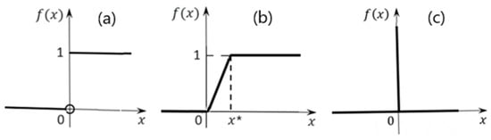
Figure 1.
Graphs of the unit jump function: (a) idealized; (b) with a transition period; and (c) delta functions ( is value of ).
In practice, a sharp change in the values of the function does not occur instantly but over a certain transitional time period x* (Figure 1b). For example, an abrupt change in the exchange rate of the national currency tenge in Kazakhstan in February 2014 against the US dollar and the euro took place over several days (Table 1). The official website of the National Bank of the Republic of Kazakhstan is www.nationalbank.kz (accessed on 15 October 2023).

Table 1.
Exchange rates in Kazakhstan.
The unit jump function is the antiderivative function for the delta function (Dirac function) [36]. The delta function graph is shown in Figure 1c.
Examples of the manifestation of the unit jump function in the economy are shown in Figure 2.
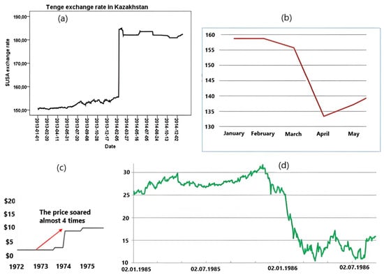
Figure 2.
Examples of abrupt changes in the economy: (a) change in the tenge exchange rate in Kazakhstan [38]; (b) the number of people employed in the USA, million people, January–May 2020 [39]; (c) WTI oil price dynamics [40]; (d) oil price from January 1985 to July 1986 [41].
In September 2020, the incidence of COVID-19 began to increase in most countries. In June 2020, the National Bureau of Economic Research (USA) announced a recession or recession in the economy since February. In absolute terms, the number of unemployed increased from 5787 people. (February) to 23,078 people. (April). In August, it amounted to 13,550 people.
In order to highlight the trend in more detail, it is possible to use a statistical procedure for smoothing the average value (Figure 3).
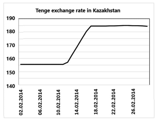
Figure 3.
Graph of the smoothed average for the change in the tenge exchange rate.
- 2.
- A unit pulse (rectangular function, normalized rectangular window) is given by the following expression:
The graph of the function is shown in Figure 4a.
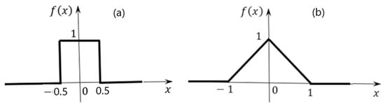
Figure 4.
Graphs of impulse functions.
- 3.
- Triangular impulse (triangular function) is a piecewise linear function given by:
The graph of the function is shown in Figure 4b.
Examples of impulse functions in the economy are shown in Figure 5.
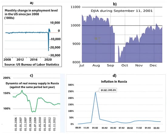
Figure 5.
Examples of impulse changes in the economy: (a) monthly change in employment level in the USA [42]; (b) Dow Jones industrial index [43]; (c) dynamics of real money supply in Russia [44]; (d) inflation in Russia [44].
The graph in Figure 5a largely corresponds to the delta function.
Figure 5b shows the macroeconomic shock caused by the 11 September 2001 terrorist attacks and is reflected in the Dow Jones Industrial Average. After the initial panic, the DJIA rose rapidly, falling only marginally from its pre-attack levels.
- 4.
- To describe rapidly changing macroeconomic processes, various combinations of impulse and jump models are possible. For example, Figure 6 shows the stepwise transformation of the Russian ruble exchange rate from one stable state to another through an impulse transition process. This shows the effect of the interaction of the step and impulse functions. The trend line is highlighted in red. Figure 7 shows the dynamics of the world cycle: industrial production, 2019–2022, and seasonally adjusted quarterly growth rates. In the figure, we see a combination of two oppositely directed impulses. It is also possible to display various variants of piecewise linear functions.
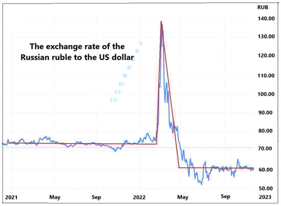 Figure 6. The exchange rate of the Russian ruble against the US dollar (blue line—initial data; red line—approximation).
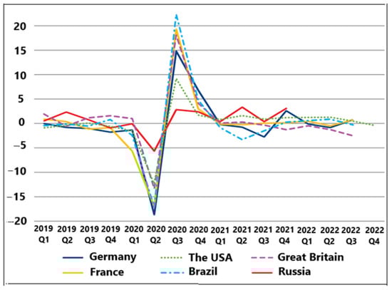 Figure 7. Dynamics of the world cycle: industrial production, 2019–2022, and seasonally adjusted quarterly growth rates [44].
3. Approximations of Step, Impulse, and Generalized Functions
3.1. Description of the Methods
Note the logical function by which a national economy (E), in general, is described, respectively:
where:
—the firms that make up the economy;
—the relationships that are constituted between firms;
—the synergy factor in the functioning of a system;
—the residual factor.
Note that the variable values in crisis states of the economy can have a spasmodic character.
It should also be noted that most economic processes are characterized by cyclical development over a fairly long period of time. The stages of cyclical development may differ (sometimes significantly) from each other, including under the influence of crisis phenomena. However, the evolution of economic processes in many cases follows a certain pattern, repeating itself after a certain period of time.
The methods developed in this article are based on the use of trigonometric functions, which, by their definition, are periodic. Consequently, these methods can be used for mathematical modeling of cyclical macroeconomic processes over a long time period. At the same time, these methods also make it possible to describe short-term, rapidly changing macroeconomic processes if these methods are used for short periods of time. In this sense, the proposed methods are universal.
Approximations of step, impulse, and generalized functions make it possible to more accurately identify trends in rapidly changing processes and describe existing processes in macroeconomics. These functional forms may become useful as predictive tools.
Currently, there are many methods for approximating piecewise linear functions using analytic expressions. This article describes only the methods proposed by the author that have a number of advantages over known approximations. These methods, like the Fourier series, are based on the use of trigonometric expressions. The difference lies in the fact that trigonometric expressions in the developed methods have the form of nested, recursive functions [45,46,47,48]. The methods were further developed in [49,50] and many other scientific papers.
Let us recall the definition of the function
For example, let us take a step function, which will explain the main idea of the approximation:
The step function is often used to describe the Fourier series. Therefore, the choice of a step function is convenient for comparing and identifying the advantages and disadvantages of expansion into the Fourier series and the methods developed by the author.
It is known that the Fourier expansion of the proposed function (1) is characterized by certain disadvantages [51,52]. The Gibbs effect can be noted. In the developed methods, the initial step function is approximated by a recursive sequence of periodic trigonometric functions, which eliminates the shortcomings of the Fourier series expansion:
The approximation sequences of function (2) are based on the interval [, ], and they are “stationary points”.
In Figure 8, the thickened line marks the initial step function. The thin lines show the graphs of five successive approximations by the proposed method. The functions are periodic; therefore, it is enough to consider them within one period. The results of studying these functions using simple mathematical transformations can be generalized to periodic functions with an arbitrary period.
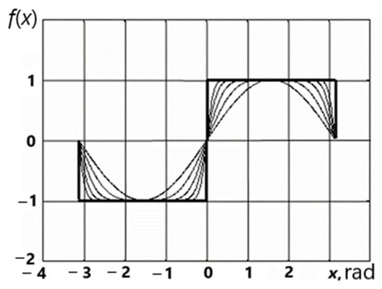
Figure 8.
Graphs of the step function (the thick line) and five successive approximations of this function (the thin lines).
Figure 8 shows that even the first approximations of the proposed iterative sequence quickly converge to the step function (1). At the same time, the shortcomings of the expansion into the Fourier series, in particular, the Gibbs effect [51], are completely leveled.
The developed methods of trigonometric approximation using an iterative recursive procedure differ in some of their properties. Let us note some of them.
Periodic functions and with period are odd. Periodic functions and are even. It follows from this fact that one can only study the approximating sequence of function (2) on the interval ; it would be enough.
Let and , because (because the function is limited) and (since the function is monotonic on the segment ); then, using Helly’s theorem, we can extract a subsequence from the given sequence . This subsequence converges to some function at each point from , and, additionally, . The original function may be such a function . Let us prove this statement.
Theorem 1.
The sequence converges pointwise to the function , but not uniformly.
Proof.
In and , there is . Therefore, since . For instance, .
for any since . has a finite limit . , or . since is increasing and positive. For , . converges at and . Therefore, . is not continuous on . Therefore, the convergence is pointwise, but not uniform. □
Theorem 2.
converges in the norm to in the spaces and .
Proof.
We take a sequence of minorant functions for :
. The measure for the set of discontinuity points of is zero. and are non-negative and limited on the segment in :
The same is true for in . □
is fundamental in and but not in .
The angular function may not necessarily be the sine, but another one, including non-periodic ones. For , . With (2), it is possible to approximate an arbitrary step function. For example, consider:
and take the function as the angular one. , , so
converges to , as shown in Figure 9.
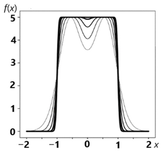
Figure 9.
Graphs of successive approximations of the bar function.
This approximating procedure makes it possible to create a mathematical analytical description of macroeconomic processes in a columnar form with arbitrary finite values of the width and height of the column. Note that the developed methods are universal and can be used to describe not only macroeconomic processes but also processes in other branches of science and technology. For example, the developed approximations of bar-shaped functions were widely used to create a new theory of semiconductors [53], and were also used in other areas.
Any step function with on can be approximated by the sum: .
where , can approximate any periodic step function. The convergence of to in the norm is ensured by the proved theorem since in and , and:
3.2. Generalized Functions and Approximation
Generalized functions [54] began to be used in the 20th century to solve problems in the field of quantum physics. The solution to such tasks required supplementing the generally recognized mathematical concept of a function. This concept suggests that with a function, we understand a certain statement; accordingly, for each value of an independent variable belonging to a certain set, one value of the dependent variable is indicated. To solve the problems of quantum physics, it was necessary to introduce functions that go beyond the usual definitions. At present, generalized functions are used not only for solving problems of quantum physics but also for solving other problems in various fields of science and engineering.
Let us consider the concept of a generalized function in more detail.
Let us take a linear space . Functions in the traditional mathematical sense are points in this space. A function is given on , and for each point from the space under consideration, we can specify a certain number. The defined function will be written , or ).
The function is linear under the assumption and continuous when follows . We consider our functions on the set of real numbers R.
A function is finite if it is equal to zero outside , and the boundaries of this segment are determined by . Any continuous function with compact support is basic. is a set of basic functions.
Next, consider a continuous function , which can have a finite number of discontinuity points. The function is bounded on any finite interval.
A function is defined by the integral . Any basic function will be finite. In this case, we have a regular function.
According to the definition in [39], any linear continuous function on is called a generalized function if:
- (α+ β)
- if in .
A generalized function that cannot be represented by the integral is called singular. For example, the δ-function or the Dirac function is a singular generalized function .
The basic idea of singular generalized functions can be visualized if we consider a generalized function from the point of view of the limit of a sequence of approximating functions with traditional definitions. In this case, generalized functions are perceived through the prism of their approximating procedures. For example, suppose:
The functions of this sequence have graphs corresponding to the graph of the step function shown in Figure 10.
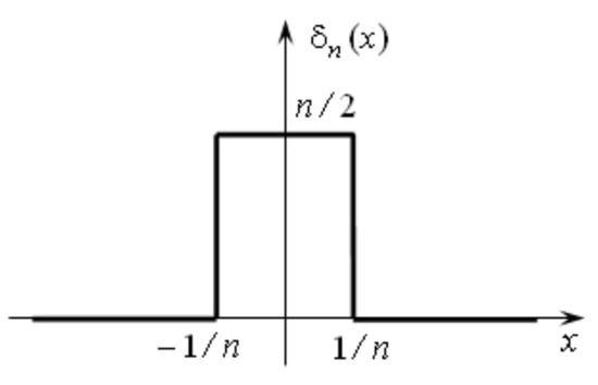
Figure 10.
Graph of the step function.
It is easy to see that for any area of the figure under the graph, the step function is equal to one.
Regarding the limit of the sequence of the functions, a graph of one of them is schematically shown in Figure 10, which is the delta function. However, step functions have discontinuity points of the first kind. At these points, the step functions are not differentiable. Therefore, this approach prevents the analytical representation of the approximation dependences for the derivatives of the delta function. Note that the derivatives of the delta function also belong to the class of generalized functions. To enable the analytical representation of derivatives, the author proposed a procedure using an approximating sequence that allows one to find derivatives of delta functions in any order. Let us write an expression that implements this approach:
For example, the graph of the function:
from the proposed sequence is shown in Figure 11.
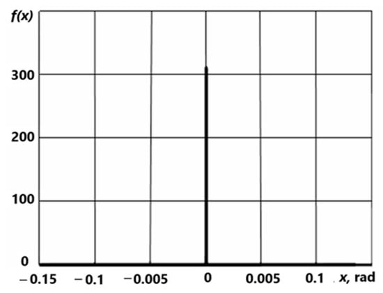
Figure 11.
Graph one of the approximations for δ-functions.
The use of cosine functions allows you to create mathematical models to describe impulse and shock macroeconomic processes. These functions allow you to make an analytical approximation of peaked functions. These cosine functions are especially useful for the mathematical modeling of auto-shock macroeconomic processes with periodically repeating impulses, the graphical representation of which resembles the so-called “Dirac comb”.
The approximation error of the δ-function by the proposed methods is much smaller compared to the Fourier series. Moreover, the approximation error can be arbitrarily small with an increase in the number of nested functions in the proposed expression. Using the integral condition written in the definition of the δ-function, one can find the amplitude of the approximation dependence.
Let us show how to find the height of the approximation peak. We know that the δ-function is the derivative of the unit jump function:
We can approximate the unit jump function (Heaviside function) by a sequence of analytic functions . The sequence is defined by (2) on ].
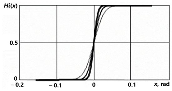
Figure 12.
Graphs of approximations of the Heaviside function.
The larger the approximation number, the greater the graph thickness (Figure 12).
Graphs of the first derivatives of successive functions are shown in Figure 13. They characterize successive approximations of the delta function.
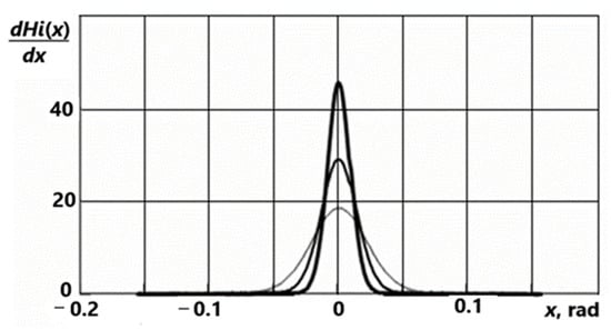
Figure 13.
Graphs of approximations for the δ-function.
For the sequence , we obtain:
Therefore, we have:
The performed analytical approximations of step, impulse, and generalized functions make it possible to use the methods of mathematical analysis in the analysis and forecasting of rapid changes in the macroeconomic situation.
The developed methods are universal and have found application in various fields of scientific research and practical applications [53,55,56,57,58,59].
4. Choice of Macroeconomic Indicators for the Analysis of Impulse and Spasmodic Processes
The totality of macroeconomic parameters is controversial. Nevertheless, it is possible to single out macroeconomic parameters, the importance of which the overwhelming majority of macroeconomists agree. We will divide the parameters into two groups (Table 2) [8]. Note that macroeconomic indicators are largely interconnected.
Table 2.
The macroeconomic parameters.
As a rule, macroeconomic indicators have annual values, in some cases, quarterly and monthly. This is the difficulty of applying macroeconomic indicators for the analysis of fast-moving (impulsive and spasmodic) economic processes. As practice shows, in some cases, the macroeconomic situation can change dramatically in a matter of days. Examples of macroeconomic indicators with daily values are the exchange rate, energy prices (and even hours and minutes) on stock exchanges, and others. Table 3, for example, shows prices for Brent crude oil.
Table 3.
Brent oil price.
The daily change in the situation on some macroeconomic indicators can be estimated indirectly. For example, the daily unemployment rate can be estimated by the number of welfare claims filed in a country during the day. Modern computer technology makes it quite easy to perform this.
To improve the accuracy of forecasting crisis situations, economic analysis should be carried out on a set of macroeconomic indicators, which provides a more holistic view of pre-crisis realities. First of all, macroeconomic indicators with greater inertia to changes are of interest. Note that macroeconomic shifts can also occur in a positive direction, which can be determined, for example, by investments and a high level of innovative development.
5. Approaches to Methods for Forecasting Macroeconomic Events
5.1. Control Rules
In quality control systems [60,61,62], control rules have been developed (Table 4), which should be paid attention to if violations of specified standards are suspected in the near future. The probability of manifestation of each of these rules within the framework of a random process is small; therefore, each of these manifestations indicates a probable violation of the course of a normal process. Therefore, with some probability, a loss of quality should be expected.
Table 4.
Control rules.
The problem of applying similar rules in the analysis of macroeconomic processes lies in the fact that in practice, changes in macroeconomic processes can occur not only for random reasons but also as a result of purposeful managerial actions. Such mathematical models do not include human behavior in the analysis, and their implications can only be intuited by macroeconomic decision-makers [11]. Therefore, for application in macroeconomic theory with impulsive and abrupt changes, these rules must be formulated with some “margin”; for example, not one value above +3 sigma but two, and not one value above + 3 sigma but one value above + 4 sigma, etc. At the same time, the probability of an error of the first kind decreases (false prediction of an impulse or abrupt development of an event series), but the probability of an error of the second kind increases (ignoring such a development). For example, Figure 14 shows graphs of the same data set in the ∓3σ range (Figure 14a) and in the ∓4σ range (Figure 14b). The range boundaries are marked with dotted lines. Some points that are critical in the range ∓3σ are not critical in the range ∓4σ. Therefore, the standard quality control rules for predicting possible crisis phenomena in the framework of the new macroeconomic theory need to be reformulated.
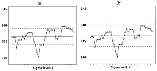
Figure 14.
Graphs of the data set in the ranges (a) ±3σ and (b) ±4σ.
Some of the rules can be left unchanged; for example, six points in a row in ascending (descending) order. This rule indicates the existence of a trend, which can lead to abrupt changes in the macroeconomic process.
The creation of a new system of rules for predicting rapid changes in macroeconomic indicators is possible on the basis of statistical processing of information and heuristic methods. Pay attention to weak signals. Note that predictions made on the basis of a system of attention-grabbing criteria can only be realized with a certain probability, which is common when using statistical methods.
In the context of the frequent lack of daily data, we will give examples of forecasts for a rapid change in macroeconomic indicators by month.
Figure 15a shows a graph of the Brent oil price (USD per barrel) for several consecutive months in 2007-08. Source of information: 1. https://investfunds.ru (accessed on 15 October 2023); 2. https://ru.investing.com (accessed on 15 October 2023). It follows in the graph that three points break the rules. Of particular interest is point number 3, since at this point three rules are violated at once (Table 5).
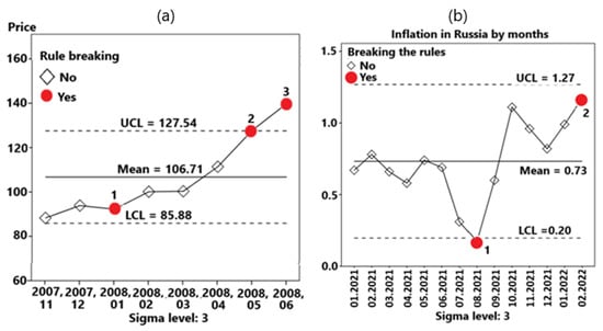
Figure 15.
Examples of completed forecasts: (a) Brent oil price (USD per barrel); (b) inflation in Russia by months as a percentage of the previous period.
Table 5.
Dynamics of oil prices.
Figure 15b shows the graph of inflation in Russia by months as a percentage of the previous period. Source of information: Rosstat data, https://rosstat.gov.ru/folder/10705 (accessed on 12 November 2023). Regarding points 1 and 2, point 2 is of particular interest since in the subsequent period (in March 2022), the inflation rate jumped sharply to a value of 7.61.
Let us take another example. Table 6 contains the values of the average monthly nominal accrued wages in rubles of employees in the whole economy of the Russian Federation. Source: Rosstat, https://rosstat.gov.ru (accessed on 12 January 2023). The December 2019 salary figure is omitted as the annual bonus is usually paid in the month of December, which greatly distorts the overall picture.
Table 6.
Average monthly salary in rubles.
A graph of the average monthly salary of points 1, 2, and 3 is shown in Figure 16.
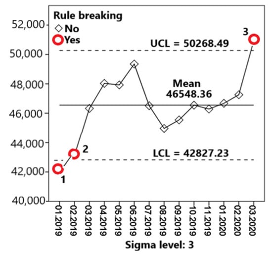
Figure 16.
Schedule of the average monthly salary.
Violation of control rules at critical points is explained in Table 7.
Table 7.
Violation of control rules.
It should be noted that in the considered examples (Figure 15 and Figure 16), the control rules of the theory of quality were applied. Within the framework of the new macroeconomic paradigm, it is necessary to revise and adjust the system of control rules based on the accumulated statistics and heuristic considerations.
We note the main issues that require further development within the framework of the new macroeconomic theory:
- Creation of a system of macroeconomic indicators with fixed daily values;
- Detailing a set of statistical rules for predicting crises and fast-moving, impulsive, and spasmodic changes in macroeconomic processes.
5.2. Theoretical Foundations of the Technique
For each macroeconomic indicator , we define:
—number of consecutive days with daily observations ;
—sample mean,
—sample standard (mean square) deviation, .
We construct the central line mean corresponding to the sample mean , and the lines ±σ, ±2σ, ±3σ, and ±4σ:
UCL—upper control limit;
LCL—lower control limit.
The upper UCL and lower LCL reference lines can correspond to values of ±3σ or ±4σ depending on our choice, as explained in Section 5.1. Next, to forecast possible abrupt changes in the macroeconomic situation, we use the control rules from Section 5.1.
As noted earlier, in order to improve the accuracy of forecasts based on the provisions of the new macroeconomic theory, macroeconomic indicators should be considered not separately, but in their totality. In this case, it is required to apply methods of multivariate analysis, such as multivariate scaling, factor analysis, cluster analysis, and others.
The new macroeconomic theory requires the accumulation of statistical data on the daily values of macroeconomic indicators due to their possible rapid change. This work is only at the beginning of the journey and requires additional effort. However, the development of computer technology does not raise doubts about the possibility of successfully solving this problem. At present, however, the overwhelming majority of macroeconomic indicators are measured by years, and only at best by quarters and months. Therefore, it is still difficult to give specific examples of forecasts based on the daily values of a set of macroeconomic indicators. It is only possible to outline some analogies of such approaches based on the annual values of macroeconomic indicators. Regarding these analogies, let us consider the dynamics of a certain set of macroeconomic indicators of the Russian Federation for the period 2012–2022 (Table 8). Source: compiled by the author based on data from the Federal State Statistics Service: https://rosstat.gov.ru/folder/10705 (accessed on 9 October 2023).
Table 8.
Dynamics of macroeconomic indicators in Russia for the period 2012–2022.
Using the ALSCAL multidimensional scaling procedure, you can obtain a visual representation of multidimensional tabular information (Figure 17a). The figure shows that 2020, 2021, and 2022 stand out sharply in terms of the totality of their indicators. Further analysis shows the economic crisis in 2020 and a sharp improvement in the situation in 2021 and 2022.
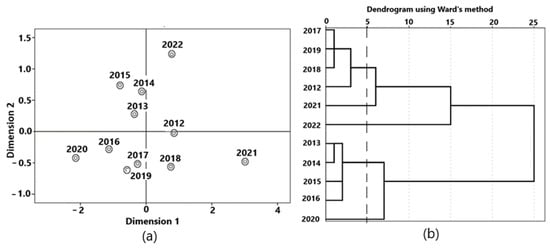
Figure 17.
Visual representation of multidimensional information: (a) multidimensional scaling; (b) cluster analysis dendrogram.
The conclusions made are confirmed by cluster analysis. Figure 17b is a dendrogram showing the possibility of splitting the variable “Year” into five clusters (section along the dotted line).
Clustering is presented in Table 9. The average values of variables by clusters are presented in Table 10.
Table 9.
Clustering.
Table 10.
Mean values of variables by clusters.
Multidimensional scaling methods have a great advantage, as they allow you to process multidimensional information and present the results of processing visually. This allows the use of macroeconomic variables in their totality to identify possible pre-crisis and forecast other rapidly changing macroeconomic situations. In addition to the previous examples, let us consider a more complete set of Russia’s macroeconomic indicators in the dynamics of their changes over the period 2004–2011 (Table 11).
Table 11.
Dynamics of the main macroeconomic indicators of Russia in 2004–2011 (growth rate, %). Source: Rosstat and the Bank of Russia.
A visual representation of the results of applying multidimensional scaling is given in Figure 18.
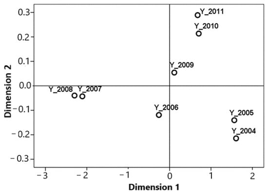
Figure 18.
Graphical representation of the results of multivariate scaling.
It can be seen in the figure that the years 2005 and 2005, 2007 and 2008, and 2010 and 2011 are pairwise close in terms of the totality of initial macroeconomic indicators. The years 2006 and 2009 occupy rather isolated positions and, therefore, differ from the rest and each other.
A similar processing of information for predicting rapid macroeconomic changes is assumed in the framework of the new macroeconomic theory in the presence of a set of variables with daily values and daily monitoring.
Currently, work is also underway to improve the mechanism of foresight control [63,64,65].
6. Discussion
- 1.
- Modern macroeconomic processes are significantly influenced by social, political, economic, and other types of crises, which are highly relevant in today’s fast-paced economic environment. The new economic paradigm urgently requires the creation of a macroeconomic theory based on new principles. Undoubtedly, such a task is complex, and its solution can only be obtained through more theoretical and empirical research. Nevertheless, it is possible and necessary to outline some approaches to creating such a theory.
To provide a practical substantiation of these statements, this article provides numerous real examples in the field of macroeconomics, illustrating rapid changes (shock, impulse, step, shift, and others) in the values of macroeconomic indicators. Mathematical descriptions of such variables are usually performed using piecewise linear functions, the types of which are presented in the article. These functions often have discontinuities, making it difficult to analyze such functions. It is necessary to consider these functions by section, and the problem arises of coordinating the obtained solutions by sections to obtain a solution for the entire process as a whole. This article describes new methods of analytical approximations of piecewise linear functions that allow us to solve this problem for mathematical modeling of rapidly changing macroeconomic processes.
In addition, this article describes, in detail, with examples, statistical approaches for the analysis of rapidly changing macroeconomic processes and their forecasting. A methodology for the practical use of these statistical approaches is presented, and recommendations are given for further improvement of the proposed approaches and methods.
- 2.
- From a theoretical point of view, the value of this article lies in the description of new approaches to macroeconomic theory, taking into account the reflection of modern conditions, characterized by crisis and rapidly changing processes. The creation of such a theory will make it possible with some probability to predict rapid changes in macroeconomic indicators and make proactive management decisions to reduce the possible negative consequences of such changes. Potential beneficiaries of the research and further development of the new macroeconomic theory may include, for example, government experts from major countries in the world, large companies, banks, investment funds, software companies, etc.
To improve the theory and methods of its practical use, it would be advisable to take into account the behavior of people and social groups and their response to rapidly changing modern macroeconomic processes. In addition, we note that the developed models can be used as the basis for artificial intelligence methods. In this sense, the developed approaches and methods of artificial intelligence do not contradict but help each other.
7. Conclusions
- This article describes only the basic approaches to mathematical modeling of macroeconomic processes with rapidly changing characteristics of the impulse and spasmodic type and formulates the main provisions of the developed model. These provisions need further development and improvement based on statistical analysis.
- The modern macroeconomic paradigm is characterized by rapid impulsive and abrupt changes, in some cases within a few days, so the analysis of macroeconomic processes should be based on the analysis of macroeconomic characteristics with daily values.
- For daily monitoring of the macroeconomic situation within the framework of the developed model, it is necessary to create a system for daily collection and processing of macroeconomic information, which can be performed on the basis of automated systems with the widespread use of computer technology.
- Daily values of macroeconomic indicators are best expressed in relative values, in the form of the dynamics of their changes for comparative analysis and identification of critical points.
- It is necessary to clarify the system of criteria for predicting possible rapid changes in the macroeconomy and identifying critical points. This may require expanded ranges of acceptable changes compared to traditional statistical methods and control rules; for example, a point falling outside the ∓4σ range, with not one but several points falling outside the ∓3σ range. The system of criteria may include rules, such as several (6 or 8) points in a row in ascending (or descending) order, to identify an emerging trend, and other control rules. Improvement of the system should be carried out using accumulated statistics of rapidly changing macroeconomic processes and heuristic methods and rules.
- To increase the accuracy of forecasts using the developed methods, macroeconomic indicators should be considered not separately but in their totality. At the same time, to identify pre-crisis conditions and possible rapid positive changes, methods of multidimensional information processing, for example, multidimensional scaling, cluster analysis, factor analysis, and others, can be useful.
- This article describes the methods developed by the author for the analytical approximation of step and generalized functions, which make it possible to describe impulse and jump functions using traditional methods of mathematical analysis. This reveals the successive connection between the developed and existing methods of macroeconomic analysis.
Funding
This research received no external funding.
Institutional Review Board Statement
Not applicable.
Informed Consent Statement
Not applicable.
Data Availability Statement
Data are available upon request.
Acknowledgments
The author thanks South Ural State University (SUSU) for its support.
Conflicts of Interest
The author declares no conflicts of interest.
References
- Weil, D.N. Economic Growth, 2nd ed.; Addison Wesley Press: New York, NY, USA, 2009; 565p. [Google Scholar]
- Solow, R.A. Contribution to the Theory of Economic Growth. Q. J. Econ. 1956, 70, 65–94. [Google Scholar] [CrossRef]
- Akaev, A.A. Models of AN-type innovative endogenous growth and their substantiation. Modernization. Innovation. Res. 2015, 6, 70–79. [Google Scholar] [CrossRef]
- LeClair, D. Technological Change, Economic Growth, and Business Education. Available online: https://gbsn.org/technological-change-economic-growth-and-business-education (accessed on 25 November 2023).
- Mankiw, N.E.; Romer, D.; Weil, D.N. A contribution to the empirics of economic growth. Q. J. Econ. 1992, 107, 407–437. [Google Scholar] [CrossRef]
- Stokey, N.; Lucas, R.; Prescott, E. Recursive Methods in Economic Dynamics; Harvard University Press: Cambridge, MA, USA, 1989. [Google Scholar]
- Bellman, R. Dynamic Programming; Princeton University Press: Princeton, NJ, USA, 1957. [Google Scholar]
- Samuelson, P.A.; Nordhaus, W.D. Economics: An Introductory Analysis, 19th ed.; McGraw–Hill: New York, NY, USA, 2009. [Google Scholar]
- Samuelson, P.A. Economic Theory and Mathematics—An Appraisal. Am. Econ. Rev. 1952, 42, 56–66. [Google Scholar]
- Samuelson, P.A. Foundations of Economic Analysis, Enlarged ed.; Harvard University Press: Cambridge, MA, USA, 1983; 604p. [Google Scholar]
- Becker, G.S. The Economic Approach to Human Behavior; University of Chicago Press: Chicago, IL, USA, 1976; 314p. [Google Scholar]
- Becker, G.S. Economic Theory; distributed by Random House; Knopf: New York, NY, USA, 1971; 222p. [Google Scholar]
- Becker, G.S. Human Capital: A Theoretical and Empirical Analysis, with Special Reference to Education, 2nd ed.; National Bureau of Economic Research, Inc.: Cambridge, MA, USA, 1975; 268p. [Google Scholar]
- Hansen, G.D.; Ohanian, L.E. Chapter 26—Neoclassical Models in Macroeconomics, Handbook of Macroeconomics; Elsevier: Amsterdam, The Netherlands, 2016; Volume 2, pp. 2043–2130. [Google Scholar]
- Pilipenko, Z.A.; Savenkova, E.V.; Pilipenko, A.I.; Morosova, E.A.; Pilipenko, O.I. Impulse Transmission Model of Macroeconomic Cycle Within the Framework of the Theory of Shocks: Aspect of Economic Security. In Dependability Engineering and Complex Systems: Proceedings of the Eleventh International Conference on Dependability and Complex Systems DepCoS-RELCOMEX, Brunów, Poland, 27 June–1 July 2016; Springer: Cham, Switzerland, 2016; Volume 470. [Google Scholar] [CrossRef]
- Basu, S.; Bundick, B. Uncertainty Shocks in a Model of Effective Demand; Working Papers, no. 12–15; Federal Reserve Bank of Boston: Boston, MA, USA, 2012. [Google Scholar]
- Barsky, R.B.; Basu, S.; Lee, K. Whither News Shocks? NBER Macroecon. Annu. 2014, 29, 225–264. [Google Scholar] [CrossRef]
- Guerron, P.; Fernandez-Villaverde, J.; Rubio-Ramirez, J. Estimating Dynamic Equilibrium Models with Stochastic Volatility. Forthcom. J. Econom. 2015, 185, 216–229. [Google Scholar]
- Sergeevich, S.O. Economic growth of a rapidly changing economy: Theoretical formulation. Econ. Reg. 2016, 2, 359. [Google Scholar]
- Heimberger, P. This time truly is different: The cyclical behavior of fiscal policy during the Covid-19 crisis. J. Macroecon. 2023, 76, 103522. [Google Scholar] [CrossRef]
- Acevedo, S.; Mrkaic, M.; Novta, N.; Pugacheva, E.; Topalova, P. The Effects of Weather Shocks on Economic Activity: What are the Channels of Impact? J. Macroecon. 2020, 65, 103207. [Google Scholar] [CrossRef]
- Aliukov, S.; Buleca, J. Comparative Multidimensional Analysis of the Current State of European Economies Based on the Complex of Macroeconomic Indicators. Mathematics 2022, 10, 847. [Google Scholar] [CrossRef]
- Hill, E.; St Clair, T.; Wial, H.; Wolman, H.; Atkins, P.; Blumenthal, P.; Ficenec, S.; Friedhoff, A. Economic Shocks and Regional Economic Resilience. In Urban and Regional Policy and Its Effects: Building Resilient Regions; Brookings Institution Press: Washington, DC, USA, 2012; Volume 9780815722854, pp. 193–274. [Google Scholar]
- Ramey, V.A. Macroeconomic Shocks and Their Propagation. University of California: San Diego, CA, USA. NBER, Cambridge, MA. Handbook of Macroeconomics 2016, 2, 71–162. [Google Scholar] [CrossRef]
- Bruneckiene, J.; Pekarskiene, I.; Palekiene, O.; Simanaviciene, Z. An Assessment of Socio-Economic Systems’ Resilience to Economic Shocks: The Case of Lithuanian Regions. Sustainability 2019, 11, 566. [Google Scholar] [CrossRef]
- Adelson, M. The Deeper Causes of the Financial Crisis: Mortgages Alone Cannot Explain It. 2013. Available online: http://www.bfjlaward.com/pdf/25892/16-31_Adelson_JPM_0412.pdf (accessed on 12 September 2023).
- Ginevicius, R.; Gedvilaite, D.; Stasiukynas, A.; Sliogeriene, J. Quantitative Assessment of the Dynamics of the Economic Development of Socioeconomic Systems Based on the MDD Method. Inz. Ekon.-Eng. Eco. 2018, 29, 264–271. [Google Scholar] [CrossRef]
- Bazzi, S.; Blattman, C. Economic Shocks and Conflict: Evidence from Commodity Prices. Am. Econ. J. Macroecon. 2014, 6, 1–38. [Google Scholar] [CrossRef]
- Ciccone, A. Economic Shocks and Civil Conflict: A Comment. Am. Econ. J. Appl. Econ. 2011, 3, 215–227. [Google Scholar] [CrossRef]
- Wardley-Kershaw, J.; Schenk-Hoppé, K.R. Economic Growth in the UK: Growth’s Battle with Crisis. Histories 2022, 2, 28. [Google Scholar] [CrossRef]
- Iuga, I.C.; Mihalciuc, A. Major Crises of the XXIst Century and Impact on Economic Growth. Sustainability 2020, 12, 9373. [Google Scholar] [CrossRef]
- Novo-Corti, I.; Țîrcă, D.-M.; Ziolo, M.; Picatoste, X. Social Effects of Economic Crisis: Risk of Exclusion. An Overview of the European Context. Sustainability 2019, 11, 336. [Google Scholar] [CrossRef]
- Murphy, R. Explaining Inflation in the Aftermath of the Great Recession. J. Macroecon. 2014, 40, 228–244. [Google Scholar] [CrossRef]
- Zagashvili, Y.V.; Rudenko, V.G. “Dynamic Characteristics of Piezogenerators” News of higher educational institutions. Instrumentation 2021, 64, 626–637. [Google Scholar]
- Plotnikov, V.A.; Makarov, S.V.; Kolubaev, E.A. Spasmodic Deformation and Pulsed Acoustic Emission under Loading of Aluminum-Magnesium Alloys. News Altai State Univ. 2014, N 1–2, 207–210. [Google Scholar]
- Koldunov, E.D.; Filonova, E.S. Econometric Modeling of Impulse Response of Macroeconomic Indicators. Fundam. Res. 2022, 6, 5–10. Available online: https://fundamental-research.ru/ru/article/view?id=43264 (accessed on 19 July 2023).
- Brylina, O.G. Static and dynamic spectral characteristics of a multi-zone converter with frequency-width-pulse modulation. Bull. South Ural. State Univ. Ser. Power Eng. 2013, 13, 70–79. [Google Scholar]
- Available online: www.nationalbank.kz (accessed on 24 November 2023).
- Available online: https://www.bls.gov (accessed on 21 September 2020).
- Available online: https://fred.stlouisfed.org/ (accessed on 17 October 2023).
- Available online: http://geoinform.ru/sem-s-polovinoj-tysyach-slancevyx-skvazhin-zhdut-svoego-chasa (accessed on 12 September 2023).
- Available online: https://catalog.archives.gov/id/584 (accessed on 12 October 2023).
- Available online: https://www.economicportal.ru/ponyatiya-all/makroekonomicheskij-shok.html (accessed on 12 September 2023).
- Available online: https://rosstat.gov.ru/ (accessed on 12 September 2023).
- Alyukov, S.V. Approximation of step functions in problems of mathematical modeling. Math. Model Comput. Simul. 2011, 3, 661–669. [Google Scholar] [CrossRef]
- Alyukov, S.V. Modeling of dynamic processes with piecewise linear characteristics, Izvestiya Vysshikh Uchebnykh Zavedenii. Appl. Nonlinear Dyn. 2011, 19, 27–34. [Google Scholar]
- Alyukov, S.V. Dynamics of Inertial Stepless Automatic Transmissions; INFRA-M: Moscow, Russia, 2013; 251p. [Google Scholar]
- Alyukov, S.V. Approximation of generalized functions and their derivatives. Questions of atomic science and technology. Series: Mathematical modeling of physical processes. Sarov: Russian Federal Nuclear Center—VNIIEF. Ser. Math. Model. Phys. Process 2013, 2, 57–62. [Google Scholar]
- Alyukov, S.V. A new method for the analytical approximation of the Heaviside function. Mod. Sci. Bull. 2013, 12, 7–10. [Google Scholar]
- Aliukov, S.; Alabugin, A.; Osintsev, K. Review of Methods, Applications and Publications on the Approximation of Piecewise Linear and Generalized Functions. Mathematics 2022, 10, 3023. [Google Scholar] [CrossRef]
- Helmberg, G. The Gibbs phenomenon for Fourier interpolation. J. Approx. Theory 1994, 78, 41–63. [Google Scholar] [CrossRef]
- Zhuk, V.V.; Natanson, G.I. Trigonometric Fourier Series and Elements of Approximation Theory; L.: Publishing House Leningrad University: Saint Petersburg, Russia, 1983; 188p. [Google Scholar]
- Seregina, E.V.; Stepovich, M.A.; Makarenkov, A.M. On the modification of a model of minority charge-carrier diffusion in semiconductor materials based on the use of recursive trigonometric functions and the estimation of the stability of solutions for the modified model. J. Synch. Investig. 2014, 8, 922–925. [Google Scholar] [CrossRef]
- Arfken, G.B.; Weber, H.J. Mathematical Methods for Physicists, 5th ed.; Academic Press: Boston, MA, USA, 2000; ISBN 978-0-12-059825-0. [Google Scholar]
- Osintsev, K.V.; Aliukov, S.V. Experimental Investigation into the Exergy Loss of a Ground Heat Pump and its Optimization Based on Approximation of Piecewise Linear Functions. J. Eng. Phys. Thermophy 2022, 95, 9–19. [Google Scholar] [CrossRef]
- Osintsev, K.V.; Aliukov, S.V. Mathematical modeling of discontinuous gas-dynamic flows using a new approximation method, Materials Science. Energy 2020, 26, 41–55. [Google Scholar] [CrossRef]
- Cai, W. Implementation of Mathematical Modeling Teaching Based on Intelligent Algorithm. In Proceedings of the ICISCAE’21, Dalian, China, 24–26 September 2021; pp. 622–626. [Google Scholar]
- Aliukov, S. Approximation of Electrocardiograms with Help of New Mathematical Methods. Comput. Math. Model. 2018, 29, 59–70. [Google Scholar] [CrossRef]
- Ubaru, S.; Saad, Y. Fast Methods for Estimating the Numerical Rank of Large Matrices. Department of Computer Science and Engineering, University of Minnesota, Twin Cities, MN USA. In Proceedings of the 33rd International Conference on Machine Learning, New York, NY, USA, 19–24 June 2016; Volume 48. [Google Scholar]
- Putri BA, D.; Handayani, D. Analysis of Product Quality Control using Six Sigma Method. In IOP Conference Series: Materials Science and Engineering; IOP Publishing: New York, NY, USA, 2019; Volume 697, p. 012005. [Google Scholar] [CrossRef]
- Thakur, V.; Akerele, O.A.; Brake, N.; Wiscombe, M.; Broderick, S.; Campbell, E.; Randell, E. Use of a Lean Six Sigma approach to investigate excessive quality control (QC) material use and resulting costs. Clin. Biochem. 2023, 112, 53–60. [Google Scholar] [CrossRef] [PubMed]
- Krotov, M.; Mathrani, S.K. A Six Sigma Approach Towards Improving Quality Management in Manufacturing of Nutritional Products. J. Ind. Eng. Manag. Sci. 2017, 1, 225–240. [Google Scholar] [CrossRef]
- Alabugin, A.; Aliukov, S.; Khudyakova, T. Models and Methods of Formation of the Foresight-Controlling Mechanism. Sustainability 2022, 14, 9899. [Google Scholar] [CrossRef]
- Alabugin, A.; Aliukov, S. Modeling Regulation of Economic Sustainability in Energy Systems with Diversified Resources. Science 2020, 3, 15. [Google Scholar] [CrossRef]
- Alabugin, A.; Aliukov, S.; Khudyakova, T. Review of Models for Socioeconomic Approaches to the Formation of Foresight Control Mechanisms: Agenesis. Sustainability 2022, 14, 11932. [Google Scholar] [CrossRef]
Disclaimer/Publisher’s Note: The statements, opinions and data contained in all publications are solely those of the individual author(s) and contributor(s) and not of MDPI and/or the editor(s). MDPI and/or the editor(s) disclaim responsibility for any injury to people or property resulting from any ideas, methods, instructions or products referred to in the content. |
© 2023 by the author. Licensee MDPI, Basel, Switzerland. This article is an open access article distributed under the terms and conditions of the Creative Commons Attribution (CC BY) license (https://creativecommons.org/licenses/by/4.0/).