Abstract
The world has been fighting against the COVID-19 Coronavirus which seems to be constantly mutating. The present wave of COVID-19 illness is caused by the Omicron variant of the coronavirus. The vaccines against the five variants (α, β, γ, δ, and ω) have been quickly developed using mRNA technology. The efficacy of the vaccine developed for one of the strains is not the same as the efficacy of the vaccine developed for the other strains. In this study, a mathematical model of the spread of COVID-19 was made by considering asymptomatic population, symptomatic population, two infected populations and quarantined population. An analysis of basic reproduction numbers was made using the next-generation matrix method. Global asymptotic stability analysis was made using the Lyapunov theory to measure stability, showing an equilibrium point’s stability, and examining the model with the fact of COVID-19 spread in Thailand. Moreover, an analysis of the sensitivity values of the basic reproduction numbers was made to verify the parameters affecting the spread. It was found that the most common parameter affecting the spread was the initial number in the population. Optimal control problems and social distancing strategies in conjunction with mask-wearing and vaccination control strategies were determined to find strategies to give better control of the spread of disease. Lagrangian and Hamiltonian functions were employed to determine the objective function. Pontryagin’s maximum principle was employed to verify the existence of the optimal control. According to the study, the use of social distancing in conjunction with mask-wearing and vaccination control strategies was able to achieve optimal control rather than controlling just one or another.
MSC:
37M05
1. Introduction
COVID-19 was first reported in December 2019 [1,2,3,4,5,6], and people all over the world have faced the challenges of the COVID-19 public health crisis. Their way of life and their economy [7] were affected since the governments needed to issue many lockdown measures to reduce the spread. Shops, department stores, and many places were closed down. Meanwhile, the use of social distancing for participating in social activities was employed to reduce the disease spread. Coronavirus disease 2019 or COVID-19 is a contagious disease caused by the virus severe acute respiratory syndrome Coronavirus 2 or SARS-CoV-2 [8,9,10,11,12,13,14,15,16], affecting the human respiratory system. COVID-19 virus can spread via droplets via from coughing, sneezing, and exposure to body secretions. The most common symptoms found among people infected with COVID-19 are cough, sore throat, runny nose or nasal congestion, loss of smell and taste, and breath difficulty, some people have severe pneumonia which sometimes can lead to death. The incubation period of COVID-19 is 2–14 days after getting the virus [11,12,17,18,19]. COVID-19 virus is one of the most widely mutating viruses. The World Health Organization (WHO) identified all five Coronavirus variants, i.e., Alpha, Beta, Gamma, Delta, and more recently Omicron [19,20]. The Omicron COVID-19 variant was first found in South Africa towards the end of November 2021 [21,22,23] and Thailand detected its first case of Omicron at the beginning of January 2022. The Omicron variant has more than 50 mutations, compared to SARS-CoV-2 [22,23], and spreads significantly faster. Therefore, its spread has to be closely monitored.
The World Health Organization (WHO) reported the worldwide spread of COVID-19. As of 31 May 2023 the total number of confirmed COVID-19 cases globally was 767.36 million and the total number of COVID-19 deaths globally was 6.93 million. As for cumulative confirmed COVID-19 cases by world region, Europe had 276.46 million, Western Pacific had 203.87 million, Americans had 192.94 million, Eastern Mediterranean had 23.37 million, and Africa had 9.53 million. The top three countries with the highest number of confirmed COVID-19 cases were the United States of America (103.43 million cases), China (99.28 million cases), and India (44.99 million cases). The top three countries with the greatest number of COVID-19 deaths were the United States of America (1.12 million deaths), Brazil (702,000 deaths) and India (531,000 deaths) [24]. In Thailand, from 3 Jan 2020 to 31 May 2023, there were 4.73 million confirmed COVID-19 cases and 34,000 COVID-19 deaths [25]. Though the number of COVID-19 patients significantly decreased, the importance given to how to reduce the number of patients is necessary to reduce the spread of the disease. Social distancing, quarantine, and vaccination are effective measures that help control the outbreak and reduce the spread of the disease [10,26,27,28,29]. According to WHO’s report on 29 May 2023, 1.33 billion doses of COVID-19 vaccines were given to people, and people in Thailand were given 139.17 million doses of COVID-19 vaccines. Vaccination is a measure that helps control the outbreak effectively.
In order to manage the COVID-19 pandemic, a mathematical model is employed to analyze situations and formulate policies to reduce the disease spread. Numerous researchers proposed different models of the spread of COVID-19 to investigate dynamics of COVID-19 spread. Lamwong et al. [30] proposed a SEIQR mathematical model for MERS-CoV by considering two groups of the population, namely, a group of the Thai population and a group of tourists from South Korea traveling to Thailand to see the effects of infections introduced by tourists. Sardar et al. [31] created a mathematical model for MERS-CoV infection based on the spread of two variants by monitoring social behavior to investigate and predict an outbreak during 2012–2016. Mwalili et al. [32] created a COVID-19 model based on the SEIR model by considering pathogens in the environment and social distancing. It was found that non-adherence to social distancing may contribute to an outbreak while quarantine for infectious individuals can help stop the spread. Yohanres et al. [33] proposed a SEIR model to describe the spread of COVID-19. An optimal measure was used to reduce the number of infectious patients, to reduce expenses spent on vaccines, and to reduce medical expenditures as much as possible. It was found that getting vaccinated for COVID-19 could decrease the number of risk groups and infectious people, showing that vaccination can control the spread of COVID-19. Omame et al. [34] made a mathematical model for the co-interaction of COVID-19 and dengue transmission dynamics in Brazil. There were five strategies used to control dengue and COVID-19 infection, namely, the prevention strategy for dengue infection, the control strategy for COVID-19 situation, the control strategy for co-infection for both dengue and COVID-19, the control strategy for dengue treatments, and the control strategy for COVID-19 treatments. It could be concluded that the prevention strategy for dengue infection could prevent COVID-19 infection among 870,000 new cases while controls against dengue and controls against COVID-19 could only considerably reduce the infection. Nainggolan and Ansori [35] studied a model of the spread of COVID-19 in Indonesia. Importance was given to quarantine for infectious persons. Parameters were examined and it was found that parameters affecting the spread were the recruitment rate, the transmission rate, and mortality rate of disease. Akuk et al. [11] proposed a mathematical model in the form of the SV1V2EQITR model. Importance was given to quarantine for infectious individuals and getting vaccinated with two doses. Stability of the model was analyzed and sensitivity of parameters affecting the spread was considered. Satar and Naji [17] proposed a mathematical model replicating the spread of the coronavirus disease by considering asymptomatic infected people. The SEIJR model (S = susceptible, E = Exposed, I = symptomatic, J = asymptomatic, and R = Recovered) was used to meet the data. Sensitivity of parameters were defined by the factors that regulate illness breakout, from the above mentioned. In this paper, we develop the model by considering additional the quarantined population to suit the epidemic situation in Thailand.
According to the literature review of articles relevant to the spread of COVID-19, a mathematical model of COVID-19 in Thailand was made. Optimal control strategies that will help control the spread of the disease were determined. From the above mentioned, the model is suitable for the epidemic situation in Thailand. Therefore, we created a model by considering the symptoms, infected population, asymptomatic, infected population, and paying attention to the population group that is in quarantine. In Section 2, the analysis of theoretical results and the analysis of disease stability were presented. In Section 3, numerical results were presented, using model fitting to estimate the results of the model to meet the actual data of the spread of the disease in Thailand. Meanwhile, the sensitivity of parameters was analyzed to examine parameters affecting the spread. In Section 4 and Section 5, optimal control strategies were presented as well as a numerical model of control strategies. A model without the determination of control strategies and a model with the determination of control strategies were compared. The research conclusion and recommendation were presented in Section 6.
2. Materials and Methods
2.1. Mathematical Model
A mathematical model is a technique to help analyze the spread of a disease and see the consequences of any actions which could be taken to prevent the spread. It is a guideline to help the government formulate policies to reduce the number of patients. The model used in the study was based on the SEIR model (Wickramaarachchi and Perera [13], Mahardika [33], Carcione et al. [36]) and the SEIQR model (Bhadauria et al. [37], Youssef et al. [38], Hussain et al. [39], Khan et al. [40], Li et al. [41], Abioye et al. [42]). As the government had a quarantine measure among infectious individuals so as to separate them from those without COVID-19, we will be concerned with the additional steps which might be taken. Therefore, the model was developed to meet the current situation. A mathematical model for COVID-19 was studied by separating people into six sub-classes, namely, susceptible classes, exposed classes, symptomatic classes, asymptomatic classes, quarantined classes, and recovered classes, where represents the susceptible population, represents the exposed population, represents the symptomatic, infected population with the ω variant, represents the asymptomatic, infected population with the other variant, represents the quarantined population, represents the recovered population, and represents the number of total populations.
The differential equation of the spread of COVID-19 can be written as follows:
and
where the variables and parameters of Equations (1) and (2) are defined in Table 1 and Table 2.
It was determined that susceptible people were able to become infected with COVID-19 since they received the disease from people in the symptomatic group and people in the asymptomatic group The intensity of the infection is
From Figure 1, the population inflow and population outflow in the mathematical model can be described as follows: susceptible group had one way of the population inflow, i.e., initial number in the population by while the population outflow was the flow of people to the exposed group based on the rate and the outflow of people who died of natural causes based on the rate . The exposed group had one way of the population inflow, namely, the flow of people from the susceptible group based on the rate while three ways of the population outflow were the flow of people to the symptomatic group and to the asymptomatic group based on the rate and the rate, respectively. The outflow of population who died of natural causes was based on the rate In the symptomatic group , there was population inflow from the exposed group to the symptomatic group based on the rate . The population outflow was the flow of people to the quarantined group based on the rate since the government had a measure ordering infected people to stay in quarantine to separate infected people from people who were not infected with the disease. Two ways of the population outflows were the outflow of people who died of natural causes and people who died of COVID-19 based on the rate and , respectively. The asymptomatic group had one way of the population inflow, i.e., the flow of people from the exposed group based on the rate . There were three ways of the population outflow, namely, the flow of people to the recovered group based on the rate deaths caused by natural causes based on the rate , and deaths caused by COVID-19 based on the rate In the quarantined group , there was population inflow, namely, the flow of people from the symptomatic group to the quarantined group based on the rate . There were two ways of population outflow, namely, the flow of people to the recovered group based on the rate and deaths caused by natural causes based on the rate The last one was the recovered group . There were two ways of population inflow, namely, the quarantined group and the asymptomatic group based on the rate and the rate, respectively. There was one way of population outflow, namely, deaths caused by natural causes based on the rate According to the above description, a differential equation of the spread of COVID-19 can be written as follows:
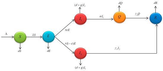
Figure 1.
Shows the relationship between population inflow and population outflow in the mathematical model of COVID-19.

Table 1.
Variables.
Table 1.
Variables.
| Variables | Description |
|---|---|
| Susceptible population. | |
| Exposed population. | |
| Symptomatic, infected population with the ω variant. | |
| Asymptomatic, infected population with the other variant. | |
| Quarantined population. | |
| Recovered population. | |
| Number of total populations. |
Table 2.
Parameters.
Table 2.
Parameters.
| Parameters | Description |
|---|---|
| The recruitment number of population. | |
| The infection rate of symptomatic population with the ω variant. | |
| The infection rate of asymptomatic population with the other variant. | |
| Incubation period. | |
| The rate of exposed moving to symptomatic. | |
| Quarantine rate of the symptomatic, infected population. | |
| Rate at which quarantine to be recovered. | |
| Rate at which asymptomatic, infected population to be recovered. | |
| Mortality rate of COVID-19. | |
| Mortality rate of natural causes. |
Lemma 1.
Initial condition:
and from the Equation (1) the invariant set and then the closed set is positive invariant.
Proof.
Groups of population are considered when , it can be seen that
From Equation (4), it is supposed that there is no mortality rate of the disease ; therefore,
integrating the above equation, it can be given as follows:
where
initial value, and
at . In addition, it can be noticed that
as . Thus, it can be concluded that
is bounded as
Epidemiological parameters are positive. It can be concluded that the problem solving area is in . Therefore
is a positive invariant set. □
2.2. Stability Analysis
2.2.1. Equilibrium Point and Basic Reproduction Number
An equilibrium point is considered in this part. An equilibrium point is important to long-term epidemic behavior since it identifies a state where the output of the system remains constant, even in the presence of varying inputs and are the states when there are no changes in the number, i.e., . Derivatives of the equation system (1) on the right side are determined to be zero. From the model, two equilibrium points are obtained, namely:
From Equation (7), we have
where
From Equation (8), we have
where
From Equation (9), we have
where
From Equation (10), we have
where
From Equation (3), we have
where
From Equation (6), we have
Therefore, or
where
Thus, when we obtain the disease-free equilibrium points , given by
Substituting and in Equation (5), we have
The remaining expressions for the endemic equilibrium points are
Therefore, disease-free equilibrium point is:
with and endemic equilibrium point is
where
with .
The value is the basic reproduction number of the equation system (1), which can be noticed from expression , and .
The next-generation matrix method [43,44] is used to derive the basic reproduction number which can be obtained from the most outstanding characteristic determinant consistent with the spectral radius of the matrix , when is spectral radius, is the Jacobian matrix of the gains matrix, and is the Jacobian matrix of the losses matrix. Then we have
It can be seen that
The disease-free equilibrium point
we have
where
Therefore, the basic reproduction number () can be derived from the most outstanding radius of considered from the largest positive eigenvalue. Thus, the formula is given as:
The basic reproduction number () represents the average number of secondary infections produced by an infected individual in a susceptible host population [45]. In an epidemiological model, if , the disease will spread and may cause an epidemic, when , an epidemic can be controlled. When is larger, an epidemic is difficult to be controlled.
2.2.2. Global Stability of Equilibrium Points
In this part, the global stability of the COVID-19 model in the equation system (1) was analyzed. The Lyapunov function was used to verify stability, and two theorems were obtained as shown below.
Theorem 1.
If , it indicates that the disease-free equilibrium point of the model (1) is globally asymptotically stable in the region .
We assume that
Proof.
According to the results shown above, the Lyapunov function was determined as follows:
The time differentiation of
is given by
using system (1), we have
substitution of the Equation (11)
based on the disease-free equilibrium point
is obtained
Therefore, it can be seen that when
and , then
Since
and
are positive. According to the Equation (15), the resul
is definitely negative. According to LaSalle’s Invariance Principle, it can be concluded that the disease-free equilibrium point
of the equation system (1) is globally asymptotically stable on if . □
Theorem 2.
If , it indicates that the endemic equilibrium point of the model (1) is globally asymptotically stable in the region .
Proof.
The Lyapunov function is determined as:
The time differentiation of
is given by
putting
and , then
An equation that is rearranged and determined is obtained.
when
and
Since all parameters in the model (1) are positive, therefore when
and
and
sultand then the re
is definitely negative when . According to LaSalle’s Invariance Principle, it can be concluded that the equilibrium point of the endemic steady state
of the equation system (1) is globally asymptotically stable on
if . □
3. Numerical Analysis Result
3.1. Model Fitting
In this part, some parameters in the model (1) were adjusted. Parameter adjustment is essential as it helps numerical simulation close to the actual data of the epidemic. Meanwhile, it helps analyze some parameters that cannot be identified. The infection rate of the symptomatic population with the ω variant the infection rate of the asymptomatic population with the other variant and the rate of exposed moving to symptomatic were adjusted as seen in Table 3. The model adjusted was implemented using fmincon Algorithm in MATLAB to ensure the model was suitable for the actual epidemic data. Results obtained from the parameter adjustment are seen in Figure 2. The blue circle indicates the number of people infected with COVID-19 each day from the data collected by the Department of Disease Control, Ministry of Public Health. The data were collected from 1 January to 1 March 2022 since the Omicron variant was confirmed. It was considered the fifth wave of COVID-19 infection [46]. The red solid line indicates results from the model (1) (susceptible group).
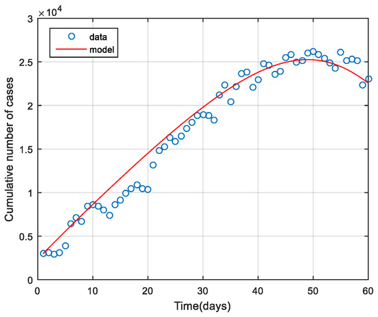
Figure 2.
Data in the model and data report in case the infection was confirmed from 1 January to 1 March 2022 [46].
3.2. Numerical Simulations
In this part, numerical analysis of the COVID-19 model (1) is performed to verify the appropriateness of the model, i.e., it yields conclusions consistent with earlier works. The Runge—Kutta order four method in MATLAB was used to generate the numerical results. The analysis in this part was divided into three parts. Part 1 is the analysis of parameter values to be suitable for the actual epidemic data. Part 2 is the analysis of model stability (1), and part 3 is the comparison of parameter values used in this study.
3.2.1. Part 1: The Analysis of Parameter Values Suitable for the Actual Epidemic Data
According to COVID-19 epidemic data reported as of 1 January to 1 March 2022 by the time the Omicron variant was confirmed in Thailand (with reference to the report on the Omicron variant detected in this when the epidemic was found the most). As for model (1), parameter values were adjusted to be suitable for the actual epidemic data. Parameters adjusted were the infection rate of the symptomatic population with the ω variant , the infection rate of the asymptomatic population with the other variant and the rate of exposed moving to symptomatic Parameter values adjusted to be suitable for the model were shown in Table 3 and Figure 2, showing appropriateness of parameters to be suitable for the actual epidemic data.
3.2.2. Part 2: Stability Analysis of the Model (1)
This part shows the numerical values of disease-free steady state, the endemic steady state, and global linear stability (globally asymptotically stable). Figure 3 shows the numerical results of a disease-free steady state. It can be seen that as time passed by, the number of susceptible 1000 days passed. The number of the exposed population the number of symptomatic, infected population the number of symptomatic, infected population the number of quarantined population and the number of recovered population as time passed by, would converge to zero (such as ) as there was no epidemic of the disease. Figure 4 shows endemic steady state of the disease. As time passed by, the number of people would converge to the equilibrium point at (11,501, 4196, 34, 6729, 137, 18,248,000) when 300 days passed. In order to see more convergence, the infection rates were adjusted to be and . The convergence was shown in the form of 2D, 3D phase portrait trajectories of model (1) as seen in Figure 5 and Figure 6. It can be seen that the convergence was clearer in both phases. Stability analysis was essential for designing an epidemiological model. If the model is stable, other controllers shall be designed (will be shown in Topic 4). If the model is not stable, it will not be used in real life and should be improved to ensure various conditions will have stability before being used.
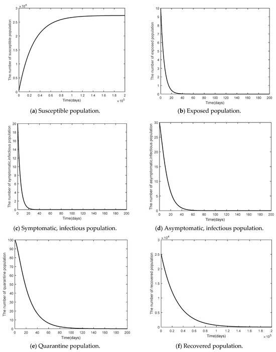
Figure 3.
Time series of the system Equation (1) of the disease-free steady state when .
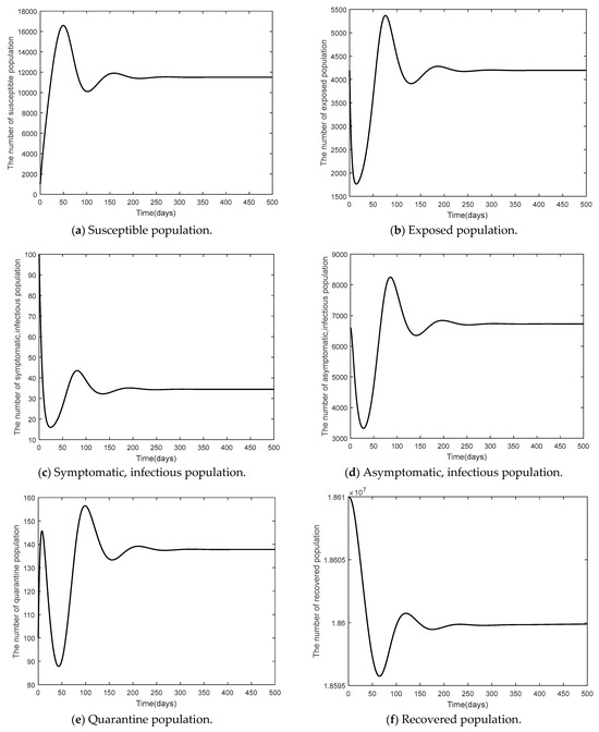
Figure 4.
Time series of the system Equation (1) of the endemic steady state when .
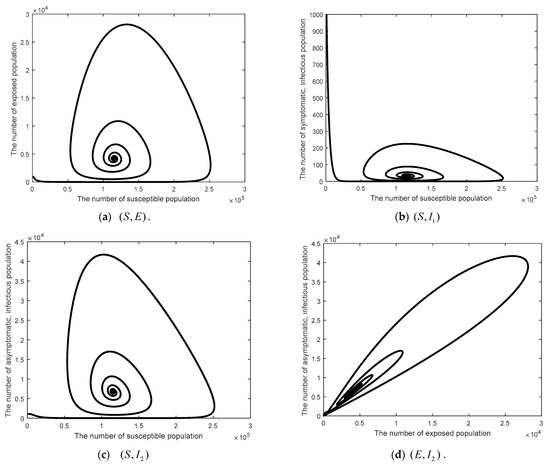
Figure 5.
Time series of the system Equation (1) projected onto the 2D of the endemic steady state when .
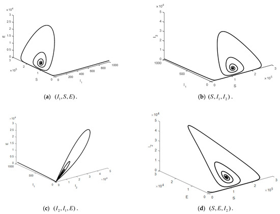
Figure 6.
Time series of the system Equation (1) projected onto the 3D of the endemic steady state when .
3.2.3. Part 3: Comparison of Parameters
The parameters used in the comparison were the initial number of people and the infection rate of the asymptomatic population with the other variant since both parameters had an impact on a high increase in the basic reproduction number , as analyzed in Table 4. The parameters adjusted were 50, 60, 70, 80 and and . From Figure 7 and Figure 8, it can be seen that increased parameter values contributed to the controllable spread of the disease rather than decreased parameter values.
Table 3.
The parameter values of model.
Table 3.
The parameter values of model.
| Parameters | Disease-Free | Endemic | Reference |
|---|---|---|---|
| 1 | 700 | Assume | |
| 0.0000075 | 0.0000075 | Fitting | |
| 0.0000009 | 0.0000009 | Fitting | |
| 1/6 | 1/6 | [36,47] | |
| 0.01 | 0.01 | Fitting | |
| 0.2 | 0.2 | [47] | |
| 0.05 | 0.05 | [47] | |
| 1/10 | 1/10 | [47] | |
| 0.00286 | 0.00286 | [47] | |
| 0.000036529 | 0.000036529 | [47,48] |
Table 4.
Sensitivity values of .
Table 4.
Sensitivity values of .
| Parameter | Sensitivity |
|---|---|
| 1 | |
| 0.000425 | |
| 0.995749 | |
| 0.000219 | |
| −0.005807 | |
| −0.004190 | |
| −0.967719 | |
| −0.027737 | |
| 1.000570 |
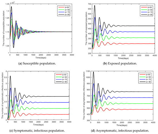
Figure 7.
Time series of the system Equation (1) showing the comparison results of initial population .
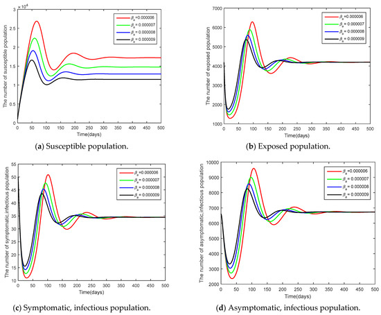
Figure 8.
Time series of the system Equation (1) showing the comparison results of the transmission rate of asymptomatic population .
3.3. Sensitivity Analysis of Parameters
In this part, sensitivity analysis for the epidemiological model is presented, aiming to learn about factors associated with the basic reproduction number the affecting numerical simulation of the model. Moreover, the sensitivity analysis will reveal the importance of each parameter affecting the epidemic. Such data would be important to designing an experimental model and help design and determine strategies for controlling the epidemic. The sensitivity index associated with the parameters is the ratio of the relative change in variables to the relative change in the parameters when variables are the function finding derivatives of parameter. The sensitivity index can be determined by the following derivatives:
Definition 1.
[10,49] The sensitivity index of , which depends differentially on a parameter , is defined by:
Expression for in Equation (13) used the data in Table 3 showing the basic value of the parameters used in the numerical simulation. Sensitivity analysis results of the basic reproduction number of each parameter are listed in Table 4.
According to the analysis results in Table 4, it can be seen that the most sensitive parameter was the initial number of the population followed by , respectively. A positive index apparently indicated an increase (or decrease) in parameter values affected an increase (or decrease) in the basic reproduction numbers (). On the contrary, indices that were negative, , led to a decrease (or increase) in the basic reproduction numbers (). The research results indicated that the most effective control strategy was controlling the initial number of the population .
4. Optimal Control Problem
Lamwong et al. [45] studied the efficiency of vaccines for COVID-19 in Thailand. It was found that a 10% increase of vaccination rates would cause a 10% increase of the basic reproduction number. It can be concluded that an increase in vaccine efficacy would cause a decreased number of infected people. However, vaccination is just one measure for controlling the spread of the disease. There may be other measures that may lessen the need for everyone to be vaccinated. These are other control steps that can be taken. In this research, optimal control strategies were presented. Control strategies introduced were and : social distancing and mask wearing strategies. vaccination control strategy to be the most suitable guideline is used with the dynamic of COVID-19 spread. Optimal control is determined as follows:
Pontryagin’s maximum principle [50,51] was used to reduce the number of COVID-19 infected people and to enable the expenditure on the control at the minimum. Therefore, the objective function was defined as follows:
Parameter represents weight constant value of infected people, represents the expenditure spent on social distancing campaign and mask wearing campaign, represents the expenditure spent on vaccination at time, and represents the last time. Nonlinear cost function was used. Squared objective function was used for cost control measurement to achieve optimal control ,
When . Lagrangian and Hamiltonian were used for optimal problem solution.
and
Theorem 3.
(Pontryagin’s Minimum Principle for control problem [44]) Optimal control was determined. and were the results of control equation system (17) that minimize over Then there exist an adjoint variable under the control equations:
And transversality conditions given as for all.
Then the characteristic values are given by
Proof.
Hamiltonian function was determined in the equation system (21).
where
is Lagrangian given in (20), therefore we have
The adjoint system satisfying the following ordinary differential equations
With transversality conditions
for all
and the optimum condition for the Hamiltonian is given as
for all
at
Therefore,
Based on the above-mentioned equation, the optimal control equation was obtained as follow:
5. Numerical Results for Optimal Control Problem
As for numerical simulation, numerical analysis of non-control model (1) and control model (19) was made. The red line indicates the non-control model, and the black line indicates the control model. The fourth order Runge—Kutta forward-backward sweep method [52] was used to generate the results. The parameters used are identified in Table 3. We have considered the initial conditions and weight constant values were determined as W2 = 20, W3 = 30, W4 = 40 and the period of the numerical simulation was determined as 100 days to ensure the goal of the control can be achieved. The highest value of the control was
. The study was divided into three cases. Case 1 is social distancing measure in conjunction with mask wearing and vaccination measure, Case 2 is social distancing measures in conjunction with mask wearing measure, and Case 3 is vaccination measures, which are described as follow:
- Case 1:
- and
It was supposed that (social distancing in conjunction with mask-wearing) and were controlled (vaccination control measure) as shown in Figure 9 and Figure 10. Figure 9 shows the results of the epidemic in the disease-free steady state and Figure 10 shows the results of the epidemic in the endemic steady state. From Figure 9 and Figure 10, it is clearly seen that social distancing measure in conjunction with mask wearing and vaccination measure were able to control the disease in a more efficient manner, compared to when no measures were available.
- Case 2:
- and
Social distancing measures were used together with mask wearing as seen in Figure 11. It can be noticed that the control measures took longer time for controlling the epidemic, compared to what happened in Case 1.
- Case 3:
- and
Only vaccination measures were used as seen in Figure 12. From Figure 12b–d, it can be seen that vaccination measures were able to control the epidemic. According to Figure 12b,c, the number of exposed people and the number of symptomatic people shall decrease and the disease can be controlled for 60 days, showing that only vaccination measures can control the epidemic similarly, compared to Case 1.
It can be said that various control measures are highly important to help control the epidemic in an efficient manner efficiently control the epidemic. Vaccination measures are considered essential for controlling the epidemic.
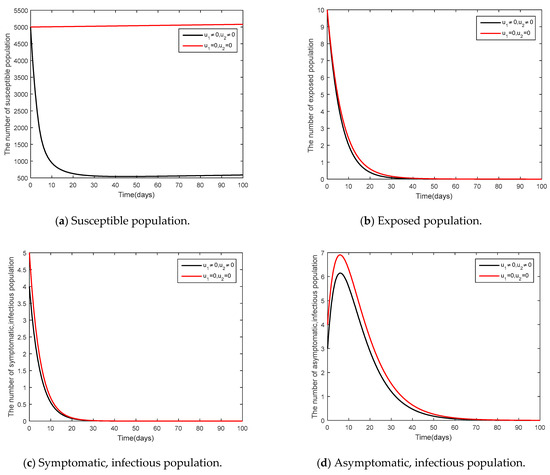
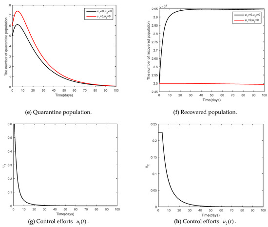
Figure 9.
Comparison between the cases and for the disease-free steady state.
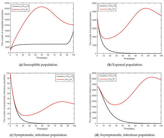
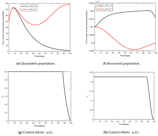
Figure 10.
Comparison between the cases and for the endemic steady state.
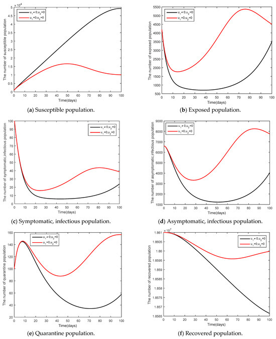
Figure 11.
Comparison between the cases and for the endemic steady state.
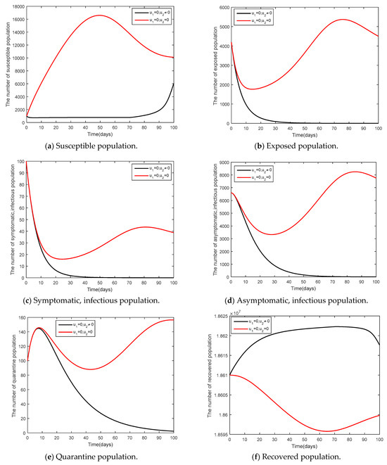
Figure 12.
Comparison between the cases and for the endemic steady state.
6. Discussion and Conclusions
This article presents a model related to the dynamic of COVID-19 spread in Thailand. According to epidemiology, a mathematical model is a tool that has been used to help analyze the spread of the fifth version of COVID-19 (Omicron). The vaccine against the α, β, γ, or δ variant of the COVID-19 coronavirus may not have the same efficacy against the ω variant. It appears the rate of infection by this variant of the coronavirus is much higher than that of the other variants and so before a new vaccine directed towards the ω variant can be developed, the other techniques to control the spread must be used. A new model must be used, one in which there are two variants are present, i.e., there are two types of infections, one caused by an α, β, γ, and δ variant of the COVID-19 coronavirus and another caused by the ω variant. A recent study by Lamwong et al. [45] studied the efficiency of vaccines for COVID-19 in Thailand. It was found that a 10% increase of vaccination rates would cause a 10% increase of the basic reproduction number. It can be concluded that an increase in vaccine efficacy would cause a decreased number of infected people. However, vaccination is just one measure for controlling the spread of the disease. There may be other measures that may lessen the need for everyone to be vaccinated. These are other control steps that can be taken. In this study, the model, developed from the model was presented. The presentation is divided into two parts. Part 1 is the non-control model. Both theoretical models and numerical analysis were available. Part 2 is the control model, developed from model (1) based on optimal control strategies to reduce the infection to the minimum. The analysis can be examined as follows:
- 1.
- Analysis of equilibrium point and the basic reproduction number of model (1). Disease-free equilibrium point , equilibrium point of endemic steady state and the basic reproduction number were calculated using the next-generation matrix method.
- 2.
- Stability analysis of model (1). The Lyapunov function was used to measure stability. It was found that in there was stability in the equilibrium point under the disease-free steady state when , and under the endemic steady state there was stability in the equilibrium point when .
- 3.
- fmincon Algorithm in MATLAB was used to be a technique for adjusting parameter values to ensure the model was suitable for the actual data of COVID-19 spread in Thailand and to estimate any spread than may come after. The parameters adjusted to be suitable for the model are the infection rate of symptomatic population , the infection rate of asymptomatic population , and the rate of exposed moving to symptomatic , making the data analysis more precise.
- 4.
- Based on the model (1), numerical data analysis was presented to verify and support theoretical conditions. The comparison of parameters found that an increase in recruitment number of people and the infection rate of asymptomatic population with the other variant had an effect on a faster control of the epidemic.
- 5.
- Parameter sensitivity analysis showed the relationship between parameter values and the basic reproduction number , indicating the importance of each parameter value affecting the epidemic. The analysis results of the model (1) are shown in Table 4. From Table 4, it can be described that positive parameter sensitivity and increased parameters affect an increase in the basic reproduction numbers, leading to an increasing epidemic. Similarly, negative parameter sensitivity and increased parameters shall affect a decrease in the basic reproduction numbers. Based on the analysis, it was found that the most sensitive parameter was the initial number of the population .
- 6.
- In this study, there were two control strategies, namely, social distancing strategy ( in conjunction with mask wearing strategy) and (vaccination control strategy). Pontryagin’s maximum principle was used to analyze the needs of conditions. The analysis was divided into three cases. Case 1 is social distancing strategy in conjunction with mask wearing strategy and vaccination control strategy, Case 2 is social distancing strategy together with mask wearing, and Case 3 is vaccination control strategy.
According to the analysis, the optimal control with the shortest duration of disease control is Case 1, social distancing strategy in conjunction with mask-wearing strategy and vaccination control strategy.
The determination of various strategies is a guideline that helps control the epidemic. There are many methods that help control the epidemic. Fractional derivatives are a tool that helps assess different outcomes and determine an optimum in a better way. It is a topic to be studied in the next chapter.
Author Contributions
Conceptualization, J.L., P.P., and N.W.; methodology, J.L.; software, N.W.; validation, J.L., P.P., I.-M.T., and N.W.; writing—original draft preparation, J.L.; writing—review and editing, J.L., P.P., I.-M.T., and N.W.; supervision, P.P., I.-M.T., and N.W.; project administration, P.P.; funding acquisition, P.P. All authors have read and agreed to the published version of the manuscript.
Funding
This work is supported by the School of Science, King Mongkut’s Institute of Technology Ladkrabang, Grant Number (2567-02-05-007).
Data Availability Statement
Data are available from the corresponding author upon reasonable request.
Acknowledgments
Jiraporn Lamwong is the recipient of the Graduate Study Fellowship of the School of Science, King Mongkut’s Institute of Technology Ladkrabang, Thailand. This research was funded by the RA-TA graduate scholarship from the School of Science, King Mongkut’s Institute of Technology Ladkrabang, grant number RA/TA-2565-D-001.
Conflicts of Interest
The authors declare that no conflicts of interest exist in the publication of this paper.
References
- Thirthar, A.A.; Abboubakar, H.; Khan, A.; Abdeljawad, T. Mathematical modeling of the COVID-19 epidemic with fear impact. AIMS Math. 2023, 8, 6447–6465. [Google Scholar] [CrossRef]
- Khan, M.A.; Atangana, A. Mathematical modeling and analysis of COVID-19: A study of new variant Omicron. Phys. A 2022, 599, 127452. [Google Scholar] [CrossRef]
- Zhang, Z.; Zeb, A.; Hussain, S.; Alzahrani, E. Dynamics of COVID-19 mathematical model with stochastic perturbation. Adv. Differ. Equ. 2020, 2020, 451. [Google Scholar] [CrossRef]
- Babaei, A.; Ahmadi, M.; Jafari, H.; Liya, A. A mathematical model to examine the effect of quarantine on the spread of coronavirus. Chaos Solitons Fractals 2021, 142, 110418. [Google Scholar] [CrossRef] [PubMed]
- Mendoza, V.M.P.; Mendoza, R.; Lee, J.; Jung, E. Managing bed capacity and timing of interventions: A COVID-19 model considering behavior and underreporting. AIMS Math. 2023, 8, 2201–2225. [Google Scholar] [CrossRef]
- Ghiasi Hafezi, S.; Seif, N.; Bahari, H.; Mohammadi, M.; Ghasemabadi, A.; Ferns, G.A.; Farkhani, E.M.; Ghayour-mobarhan, M. The association between macronutrient intakes and coronavirus disease 2019 (COVID-19) in an Iranian population: Applying a dynamical system model. J. Health Popul. Nutr. 2023, 42, 114. [Google Scholar] [CrossRef] [PubMed]
- Shen, Z.H.; Chu, Y.M.; Khan, M.A.; Al-Hartomy, O.A.; Higazy, M. Mathematical modeling and optimal control of the COVID-19 dynamics. Results Phys. 2021, 31, 105028. [Google Scholar] [CrossRef]
- Ghazizadeh, H.; Shakour, N.; Ghofchi, S.; Mansoori, A.; Saberi-Karimiam, M.; Rashidmayvan, M.; Ferns, G.; Esmaily, H.; Ghayour-Mobarhan, M. Use of data mining approaches to explore the association between type 2 diabetes mellitus with SARS-CoV-2. BMC Pulm. Med. 2023, 23, 203. [Google Scholar] [CrossRef]
- Sepulveda, G.; Arenas, A.J.; González-Parra, G. Mathematical Modeling of COVID-19 Dynamics under Two Vaccination Doses and Delay Effects. Mathematics 2023, 11, 369. [Google Scholar] [CrossRef]
- Khan, A.A.; Ullaha, S.; Amin, R. Optimal control analysis of COVID-19 vaccine epidemic model: A case study. Eur. Phys. J. Plus 2022, 137, 156. [Google Scholar] [CrossRef]
- Philip, N.A.A.; Seidu, B.; Bornaa, C.S. Mathematical Analysis of COVID-19 Transmission Dynamics Model in Ghana with Double-Dose Vaccination and Quarantine. Comput. Math. Methods Med. 2022, 2022, 7493087. [Google Scholar]
- Jankhonkhan, J.; Sawangtong, W. Model Predictive Control of COVID-19 pandemic With Social Isolation and Vaccination Policies in Thailand. Axioms 2021, 10, 274. [Google Scholar] [CrossRef]
- Wickramaarachchi, W.P.T.M.; Perera, S.S.N. An SIER model to estimate optimal transmission rate and initial parameters of COVD-19 dynamic in Sri Lanka. Alex. Eng. J. 2021, 60, 1557–1563. [Google Scholar] [CrossRef]
- Daniel, D.O. Mathematical Model for the Transmission of COVID-19 with Nonlinear Forces of Infection and the Need for Prevention Measure in Nigeria. J. Infect. Dis. Epidemiol. 2020, 6, 158. [Google Scholar]
- Veera Krishna, M.; Prakas, J. Mathematical modelling on phase based transmissibility of Coronavirus. Infect. Dis. Model. 2020, 5, 375–385. [Google Scholar] [CrossRef] [PubMed]
- Mishraa, A.M.; Purohit, S.D.; Owolabi, K.M.; Sharma, Y.D. A nonlinear epidemiological model considering asymptotic and quarantine classes for SARS CoV-2 virus. Chaos Solitons Fractals 2020, 138, 109953. [Google Scholar] [CrossRef]
- Satar, H.A.; Naji, R.K. A Mathematical Study for the Transmission of Coronavirus Disease. Mathematics 2023, 11, 2330. [Google Scholar] [CrossRef]
- Zamir, M.; Abdeljawad, T.; Nadeem, F.; Yousef, A. An optimal control analysis of a COVID-19 model. Alex. Eng. J. 2021, 60, 2875–2884. [Google Scholar] [CrossRef]
- Baba, I.A.; Nasidi, B.A.; Baleanu, D.; Saadi, S.H. A mathematical model to optimize the available control measures of COVID–19. Ecol. Complex. 2021, 46, 100930. [Google Scholar] [CrossRef]
- World Health Organization. SARS-CoV-2 Variant Tracking. Available online: https://www.who.int/fr/activities/tracking-SARS-CoV-2-variants (accessed on 31 May 2022).
- Minka, S.; Minka, F. A tabulated summary of the evidence on humoral and cellular responses to the SARS-CoV-2 Omicron VOC, as well as vaccine efficacy against this variant. Immunol. Lett. 2022, 243, 38–43. [Google Scholar] [CrossRef]
- González-Parra, G.; Arenas, A.J. Mathematical Modeling of SARS-CoV-2 Omicron Wave under Vaccination Effects. Computation 2023, 11, 36. [Google Scholar] [CrossRef]
- Martin, D.P.; Lytras, S.; Lucaci, A.G.; Maier, W.; Gruning, B.; Shank, S.D.; Weaver, S.; MacLean, O.A.; Orton, R.J.; Lemey, P.; et al. Selection Analysis Identifies Significant Mutational Changes in Omicron That Are Likely to Influence Both Antibody Neutralization and Spike Function (Part 1 of 2). Virological. Org. 2021, 5, pp. 1–2. Available online: https://virological.org/t/selection-analysis-identifies-significant-mutational-changes-in-omicron-that-are-likely-to-influence-both-antibody-neutralization-and-spike-function-part-1-of-2/771 (accessed on 10 June 2023).
- World Health Organization. WHO Coronavirus (COVID-19) Dashboard. 2023. Available online: https://covid19.who.int/ (accessed on 31 May 2022).
- World Health Organization. WHO Coronavirus (COVID-19) Dashboard. 2023. Available online: https://covid19.who.int/region/searo/country/th (accessed on 31 May 2022).
- Sun, T.-C.; DarAssi, M.H.; Alfwzan, W.F.; Khan, M.A.; Alshahrani, A.S.; Alqahtani, S.S.; Muhammad, T. Mathematical Modeling of COVID-19 with Vaccination Using Fractional Derivative: A Case Study. Fractal Fract. 2023, 7, 234. [Google Scholar] [CrossRef]
- Gumu, O.A.; Selvam, A.G.M.; Janagaraj, R.; Selvam, G.M.; Janagaraj, R. Dynamics of the Mathematical Model Related to COVID-19 Pandemic with Treatment. Thai J. Math. 2022, 20, 957–970. [Google Scholar]
- Chhetri, B.; Bhagat, V.M.; Muthusamy, S.; Ananth, V.S.; Vamsi, D.K.K.; Sanjeevi, C.B. Time Optimal Control Studies on COVID-19 Incorporating Adverse Events of the Antiviral Drugs. Comput. Math. Biophys. 2021, 9, 214–241. [Google Scholar] [CrossRef]
- Nabi, K.N.; Kumar, P.; Erturk, V.S. Projections and fractional dynamics of COVID-19 with optimal control strategies. Chaos Solitons Fractals 2021, 145, 110689. [Google Scholar] [CrossRef] [PubMed]
- Lamwong, J.; Tang, I.-M.; Pongsumpun, P. Mers Model of Thai and South Korean Population. Curr. Appl. Sci. Technol. 2018, 18, 45–57. [Google Scholar]
- Sardar, T.; Ghosh, I.; Rodo, X.; Chattopadhyay, J. A realistic two-strain model for MERS-CoV infection uncovers the high risk for epidemic propagation. PLoS Negl. Trop. Dis. 2020, 14, e0008065. [Google Scholar] [CrossRef]
- Mwalili, S.; Kimathi, M.; Ojiambo, V.; Gathungu, D.; Mbogo, R. SEIR model for COVID-19 dynamics incorporating the environment and social distancing. BMC. Res. Notes 2020, 13, 352. [Google Scholar] [CrossRef]
- Mahardika, Y.D. Dynamical Modeling of COVID-19 and Use of Optimal Control to Reduce the Infected Population and Minimize the Cost of Vaccination and Treatment. ComTech Comput. Math. Eng. Appl. 2021, 12, 65–73. [Google Scholar] [CrossRef]
- Omame, A.; Rwezaura, H.; Diagne, M.L.; Inyama, S.C.; Tchuenche, J.M. COVID-19 and dengue co-infection in Brazil: Optimal control and cost-effectiveness analysis. Eur. Phys. J. Plus 2021, 136, 1090. [Google Scholar] [CrossRef]
- Nainggolan, J.; Ansori, M.F. Stability and Sensitivity Analysis of the COVID-19 Spread with Comorbid Diseases. Symmetry 2022, 14, 2269. [Google Scholar] [CrossRef]
- Carcione, J.M.; Santos, J.E.; Bagaini, C.; Ba, J. A Simulation of a COVID-19 Epidemic Based on a Deterministic SEIR Model. Front. Public Health 2020, 8, 230. [Google Scholar] [CrossRef] [PubMed]
- Bhadauria, A.S.; Devi, S.; Nivedita, G. Modelling and analysis of a SEIQR model on COVID-19 pandemic with delay. Model. Earth Syst. Environ. 2022, 8, 3201–3214. [Google Scholar] [CrossRef] [PubMed]
- Youssef, H.; Alghamdi, N.; Ezzat, M.A.; El-Bary, A.A.; Shawky, A.M. Study on the SEIQR model and applying the epidemiological rates of COVID-19 epidemic spread in Saudi Arabia. Infect. Dis. Model. 2021, 6, 678–692. [Google Scholar] [CrossRef] [PubMed]
- Hussain, T.; Ozair, M.; Ali, F.; Rehman, S.; Assiri, T.A.; Mahmoud, E.E. Sensitivity analysis and optimal control of COVID-19 dynamics based on SEIQR model. Results Phys. 2021, 22, 103956. [Google Scholar] [CrossRef] [PubMed]
- Khan, A.; Zarin, R.; Hussain, G.; Ahmad, N.A.; Mohd, M.H.; Yusuf, A. Stability analysis and optimal control of COVID-19 with convex incidence rate in Khyber Pakhtunkhawa (Pakistan). Results. Phys. 2021, 20, 103703. [Google Scholar] [CrossRef] [PubMed]
- Li, M.-T.; Sun, G.-Q.; Zhang, J.; Zhao, Y.; Pei, X.; Li, L.; Wang, Y.; Zhang, W.-Y.; Zhang, Z.-K.; Jin, Z. Analysis of COVID-19 transmission in Shanxi Province with discrete time imported cases. Math. Biosci. Eng. 2020, 17, 3710–3720. [Google Scholar] [CrossRef]
- Abioye, A.I.; Peter, O.J.; Ogunseye, H.A.; Oguntolu, F.A.; Oshinubi, K.; Ibrahim, A.A.; Khan, I. Mathematical model of COVID-19 in Nigeria with optimal control. Results Phys. 2021, 28, 104598. [Google Scholar] [CrossRef]
- van den Driessche, P.; Watmough, J. Reproduction numbers and sub-threshold endemic equilibria for compartmental models of disease transmission. Math. Biosci. 2002, 180, 29–48. [Google Scholar] [CrossRef]
- Perkins, T.A.; España, G. Optimal Control of the COVID-19 Pandemic with Non-pharmaceutical Interventions. Bull. Math. Biol. 2020, 82, 118. [Google Scholar] [CrossRef]
- Lamwong, J.; Pongsumpun, P.; Tang, I.-M.; Wongvanich, N. Vaccination’s Role in Combating the Omicron Variant Outbreak in Thailand: An Optimal Control Approach. Mathematics 2022, 10, 3899. [Google Scholar] [CrossRef]
- World Health Organization. COVID-19—WHO Thailand Situation Reports. Available online: https://www.who.int/thailand/emergencies/novel-coronavirus-2019/situation-reports (accessed on 25 January 2023).
- Riyapan, P.; Shuaib, S.E.; Intarasit, A. A Mathematical Model of COVID-19 Pandemic: A Case Study of Bangkok, Thailand. Comput. Math. Methods Med. 2021, 2021, 6664483. [Google Scholar] [CrossRef] [PubMed]
- Alshammari, F.S. A Mathematical Model to Investigate the Transmission of COVID19 in the Kingdom of Saudi Arabia. Comput. Math. Methods Med. 2020, 2020, 1–13. [Google Scholar] [CrossRef] [PubMed]
- Bandekara, S.R.; Ghosh, M. Mathematical modeling of COVID-19 in India and Nepal with optimal control and sensitivity analysis. Eur. Phys. J. Plus 2021, 136, 1058. [Google Scholar] [CrossRef] [PubMed]
- Kamien, M.I.; Schwartz, N.L. Dynamic Optimization: The Calculus of Variations and Optimal Control in Economics and Management; Elsevier: Amsterdam, The Netherlands, 1991. [Google Scholar]
- Guo, T.; Li, Y. Modeling and optimal control of mutated COVID-19 (Delta strain) with imperfect vaccination. Chaos Solitons Fractals 2022, 156, 111825. [Google Scholar]
- Adepoju, O.A.; Samson Olaniyi, S. Stability and optimal control of a disease model with vertical transmission and saturated incidence. Sci. Afr. 2021, 12, e00800. [Google Scholar] [CrossRef]
Disclaimer/Publisher’s Note: The statements, opinions and data contained in all publications are solely those of the individual author(s) and contributor(s) and not of MDPI and/or the editor(s). MDPI and/or the editor(s) disclaim responsibility for any injury to people or property resulting from any ideas, methods, instructions or products referred to in the content. |
© 2023 by the authors. Licensee MDPI, Basel, Switzerland. This article is an open access article distributed under the terms and conditions of the Creative Commons Attribution (CC BY) license (https://creativecommons.org/licenses/by/4.0/).