Hermitian Solutions of the Quaternion Algebraic Riccati Equations through Zeroing Neural Networks with Application to Quadrotor Control

Abstract

The stability of nonlinear systems in the control domain has been extensively studied using different versions of the algebraic Riccati equation (ARE). This leads to the focus of this work: the search for the time-varying quaternion ARE (TQARE) Hermitian solution. The zeroing neural network (ZNN) method, which has shown significant success at solving time-varying problems, is used to do this. We present a novel ZNN model called ’ZQ-ARE’ that effectively solves the TQARE by finding only Hermitian solutions. The model works quite effectively, as demonstrated by one application to quadrotor control and three simulation tests. Specifically, in three simulation tests, the ZQ-ARE model finds the TQARE Hermitian solution under various initial conditions, and we also demonstrate that the convergence rate of the solution can be adjusted. Furthermore, we show that adapting the ZQ-ARE solution to the state-dependent Riccati equation (SDRE) technique stabilizes a quadrotor’s flight control system faster than the traditional differential-algebraic Riccati equation solution.

1. Introduction

Algebraic Riccati equations (AREs) have gained considerable magnitude in applied mathematics and a range of engineering issues since Kalman showed how widely used they are in filtering and optimal control theory [1]. These problems include controlling wind generators [2], linear multi-agent systems [3], and wheeled inverted pendulums [4]. In particular, the continuous-time ARE is the following quadratic matrix equation [5]:

$$A^{\mathrm{T}}X+XA-XBX+C={\mathbf{0}}_{n\times n}.$$

(1)

Linear-quadratic regulators [6,7,8], Kalman filtering [5,9], linear-quadratic-Gaussian along with $H_2$/H∞ control [10,11], and coprime and spectral factorizations [12,13] all depend on this matrix equation. It is significant to mention that ${()}^{\mathrm{T}}$ signifies transposition; the zero $p\times 1$ and $p\times n$ matrices are referred to as ${\mathbf{0}}_p$ and ${\mathbf{0}}_{p\times n}$, respectively; and each matrix in (1) belongs to ${\mathbb{R}}^{n\times n}$, with B and C being symmetric and nonnegative definite matrices (i.e., $B=B^{\mathrm{T}}\ge 0$ and $C=C^{\mathrm{T}}\ge 0$). Also, there can be an infinite or a finite number of symmetric or antisymmetric solutions X with definite or indefinite signs in the solutions set for (1).

Let $\mathbb{H}=\{{\beta }_1+{\beta }_2ı+{\beta }_{3}j+{\beta }_{4}k|{ı}^2=j^2=k^2=ıjk=-1,{\beta }_1,{\beta }_2,{\beta }_3,{\beta }_4\in \mathbb{R}\}$ be the quaternions set and ${\mathbb{H}}^{n\times n}$ be the $n\times n$ matrices set on $\mathbb{H}$ [14]. Note that quaternions are a system of non-commutative numbers that builds upon complex numbers. In this paper, a recurrent neural network, called a ’zeroing neural network (ZNN)’, is used to solve the next time-varying quaternion ARE (TQARE):

$${\tilde{A}}^{*}(t)\tilde{X}(t)+\tilde{X}(t)\tilde{A}(t)-\tilde{X}(t)\tilde{B}(t)\tilde{X}(t)+\tilde{C}(t)={\mathbf{0}}_{n\times n},$$

(2)

where all time-varying matrices are in ${\mathbb{H}}^{n\times n}$, ${()}^{*}$ denotes the conjugate transpose, and $\tilde{B}(t)$ and $\tilde{C}(t)$ are assumed to be positive semidefinite (i.e., $\tilde{B}(t)={\tilde{B}}^{*}(t)\ge 0$ and $\tilde{C}(t)={\tilde{C}}^{*}(t)\ge 0$). According to [15], there can be an infinite or a finite number of Hermitian or non-Hermitian solutions $\tilde{X}(t)$ with definite or indefinite signs in the solutions set for (2). Notably, Hamilton proposed quaternions for the first time in 1843 [16]. Since they are helpful in computations involving three-dimensional rotations in applied and theoretical mathematics [17], they are highly significant in a number of domains, such as mathematical physics [18], computer modeling [19], quantum mechanics [20], navigation [21], electromagnetism [22], and robotics [23].

The study of dynamic problems involving time-varying quaternion matrices (TVQM) has garnered more attention recently. These problems include the linear TVQM equation [24], the pseudoinverse of TVQM [25], the constrained TVQM least-squares issue [26], and the inversion of TVQM [27]. Furthermore, real-world applications of TVQMs include chaotic system synchronization [28], robot joint kinematically redundant manipulators [29], mobile manipulator control [30], picture restoration [31], and acoustic source tracking [32]. There is a commonality throughout all of these studies: they employ the ZNN method to find the response. It is noteworthy that Zhang et al. introduced the ZNN technique in [33] to address time-varying tasks in real time. ZNNs, in particular, are recurrent neural networks that perform exceptionally well at parallel processing. Dynamical systems for computing time-varying pseudoinverses were among their subsequent applications [34,35]. Nonlinear equation systems [36,37], linear equation systems [38,39], linear/quadratic programming [40,41,42], and generalized inversion [43,44] are among the challenges that they are currently utilized for. A ZNN model is typically constructed via two primary steps. Firstly, we need to define the error matrix equation (EME) $E(t)$. Secondly, the dynamical system that follows has to be used:

$$\dot{E}(t)=-\lambda E(t),$$

(3)

where $t\in [0,t_f)\subseteq [0,+\infty )$ is the time, and the time derivative operator is $(\dot{})$. Furthermore, the convergence rate of the model can be modified by varying the parameter $\lambda \in {\mathbb{R}}^{+}$. For instance, a bigger value of $\lambda$ causes any ZNN model to converge even quicker [45]. The foundation of the ZNN’s architecture is to put $E(t)$ to 0, which holds as $t\to \infty$. The real-time learning rule that results from the creation of EME in (3) is used to do this. EME can therefore be regarded as a tool for tracking model learning.

In this paper, a novel ZNN model, termed ’ZQ-ARE’, is presented for solving the TQARE by identifying only Hermitian solutions. One application to quadrotor control and three simulation experiments show that the model performs admirably. Additionally, compared to the traditional differential-algebraic Riccati equation (DARE) solution, the ZQ-ARE solution adaption to the state-dependent Riccati equation (SDRE) technique demonstrates that it stabilizes a quadrotor’s flight control system more quickly. Notice that through a theoretical analysis of the ZQ-ARE model, this study contributes to the corpus of the literature. Last, the paper’s contributions are shown in the following list.

• A novel ZNN model, termed ’ZQ-ARE’, for solving the TQARE by identifying only Hermitian solutions is introduced.
• A theoretical analysis is carried out in order to validate the ZQ-ARE model.
• Sim tests and a real-world application to quadrotor control are carried out to supplement the theoretical study.
• For the task of stabilizing the flight control system of a quadrotor, a comparison is given between the solution adaptations provided by the traditional DARE, the ZQ-ARE, and the SDRE methods.

The all-ones $p\times 1$ and $p\times n$ matrices will be indicated by ${\mathbf{1}}_p$ and ${\mathbf{1}}_{p\times n}$, respectively, while the identity $p\times p$ matrix will be indicated by $I_p$ throughout the duration of this paper. In addition, $\otimes ,\mathrm{vec}(·),\odot$ will represent the Kronecker product, the vectorization procedure, and the Hadamard product, respectively. Lastly, the matrix Frobenius norm will be represented as ${∥·∥}_{\mathrm{F}}$, and inversion and pseudoinversion will be indicated by superscripts ${()}^{-1}$ and ${()}^{†}$, respectively.

The layout of the paper is as follows. The TQARE reformulation and quaternion preliminary results are presented in Section 2. In Section 3, the ZQ-ARE model—which is grounded in the ZNN method—is described, and in Section 4, its theoretical analysis is offered. Notice that the computational complexity of the ZQ-ARE model is described in Section 3. Simulation experiments and application to quadrotor control are shown in Section 5. Section 6 wraps up with some final thoughts and observations.

2. Preliminaries and Reformulation of the TQARE

The TQARE is reformulated and the foundations of TVQM are outlined in this part. Notice that the TQARE (2) is being reformulated in order to lower the ZNN technique’s computational complexity.

Allow $\tilde{M}(t)=M_1(t)+M_2(t)ı+M_3(t)j+M_4(t)k\in {\mathbb{H}}^{n\times n}$ to represent a TVQM using the coefficient matrices $M_j(t)\in {\mathbb{R}}^{n\times n}$ for $j=1,2,3,4$. Next is the conjugate transpose of the TVQM $\tilde{M}(t)$ [14,46]:

$${\tilde{M}}^{*}(t)=M_1^{\mathrm{T}}(t)-M_2^{\mathrm{T}}(t)ı-M_3^{\mathrm{T}}(t)j-M_4^{\mathrm{T}}(t)k.$$

(4)

Similarly, consider the TVQMs $\tilde{C}(t),\tilde{X}(t),\tilde{B}(t),\tilde{A}(t)\in {\mathbb{H}}^{n\times n}$, which use the coefficient matrices $C_j(t),X_j(t),B_j(t),A_j(t)\in {\mathbb{R}}^{n\times n}$ for $j=1,2,3,4$. The following is the product of $\tilde{B}(t)$ and $\tilde{X}(t)$:

$$\tilde{B}(t)\tilde{X}(t)=\widetilde{BX}(t)=B{X}_1(t)+B{X}_2(t)ı+B{X}_3(t)j+B{X}_4(t)k\in {\mathbb{H}}^{m\times n},$$

(5)

where the following are the coefficient matrices $B{X}_j(t)\in {\mathbb{R}}^{m\times n}$:

$$\begin{array}{c}B{X}_1(t)=-B_3(t)X_3(t)+B_1(t)X_1(t)-B_2(t)X_2(t)-B_4(t)X_4(t),\\ B{X}_2(t)=B_1(t)X_2(t)+B_3(t)X_4(t)+B_2(t)X_1(t)-B_4(t)X_3(t),\\ B{X}_3(t)=B_1(t)X_3(t)+B_3(t)X_1(t)-B_2(t)X_4(t)+B_4(t)X_2(t),\\ B{X}_4(t)=B_4(t)X_1(t)+B_1(t)X_4(t)-B_3(t)X_2(t)+B_2(t)X_3(t).\end{array}$$

(6)

In the same manner, we can create the products $\widetilde{AX}(t)={\tilde{A}}^{*}(t)\tilde{X}(t)$, $\widetilde{XA}(t)=\tilde{X}(t)\tilde{A}(t)$, and $\widetilde{XBX}(t)=\tilde{X}(t)\widetilde{BX}(t)$.

Using the previously provided information, Equation (2) can be rewritten as follows:

$$\widetilde{AX}(t)+\widetilde{XA}(t)-\widetilde{XBX}(t)+\tilde{C}(t)={\mathbf{0}}_{n\times n},$$

(7)

where the following is true:

$$\left\{\begin{array}{c}\hfill A{X}_1(t)+X{A}_1(t)-XB{X}_1(t)+C_1(t)={\mathbf{0}}_{n\times n},\hfill \\ \hfill A{X}_2(t)+X{A}_2(t)-XB{X}_2(t)+C_2(t)={\mathbf{0}}_{n\times n},\hfill \\ \hfill A{X}_3(t)+X{A}_3(t)-XB{X}_3(t)+C_3(t)={\mathbf{0}}_{n\times n},\hfill \\ \hfill A{X}_4(t)+X{A}_4(t)-XB{X}_4(t)+C_4(t)={\mathbf{0}}_{n\times n}.\hfill \end{array}\right.$$

(8)

Then, setting

$$\begin{array}{c}Y(t)=\left[\begin{array}{cccc}{X}_1(t)& -X_2(t)& -X_3(t)& -X_4(t)\\ X_2(t)& X_1(t)& -X_4(t)& X_3(t)\\ X_3(t)& X_4(t)& X_1(t)& -X_2(t)\\ X_4(t)& -X_3(t)& X_2(t)& X_1(t)\end{array}\right],A(t)=\left[\begin{array}{c}{A}_1(t)\\ A_2(t)\\ A_3(t)\\ A_4(t)\end{array}\right],C(t)=\left[\begin{array}{c}{C}_1(t)\\ C_2(t)\\ C_3(t)\\ C_4(t)\end{array}\right],\\ W(t)=\left[\begin{array}{cccc}{B}_1(t)& -B_2(t)& -B_3(t)& -B_4(t)\\ B_2(t)& B_1(t)& -B_4(t)& B_3(t)\\ B_3(t)& B_4(t)& B_1(t)& -B_2(t)\\ B_4(t)& -B_3(t)& B_2(t)& B_1(t)\end{array}\right],B(t)=\left[\begin{array}{c}{B}_1(t)\\ B_2(t)\\ B_3(t)\\ B_4(t)\end{array}\right],X(t)=\left[\begin{array}{c}{X}_1(t)\\ X_2(t)\\ X_3(t)\\ X_4(t)\end{array}\right],\\ D(t)=\left[\begin{array}{cccc}{A}_1^{\mathrm{T}}(t)& A_2^{\mathrm{T}}(t)& A_3^{\mathrm{T}}(t)& A_4^{\mathrm{T}}(t)\\ -A_2^{\mathrm{T}}(t)& A_1^{\mathrm{T}}(t)& A_4^{\mathrm{T}}(t)& -A_3^{\mathrm{T}}(t)\\ -A_3^{\mathrm{T}}(t)& -A_4^{\mathrm{T}}(t)& A_1^{\mathrm{T}}(t)& A_2^{\mathrm{T}}(t)\\ -A_4^{\mathrm{T}}(t)& A_3^{\mathrm{T}}(t)& -A_2^{\mathrm{T}}(t)& A_1^{\mathrm{T}}(t)\end{array}\right],\hfill \end{array}$$

(9)

where $Y(t),W(t),D(t)\in {\mathbb{R}}^{4n\times 4n}$ and $X(t),B(t),C(t),A(t)\in {\mathbb{R}}^{4n\times n}$, Equation (7) can be reconstructed as follows:

$$D(t)X(t)+Y(t)A(t)-Y(t)W(t)X(t)+C(t)={\mathbf{0}}_{4n\times n},$$

(10)

where the coefficient matrices of $\tilde{X}(t)$, $X_j(t),j=1,2,3,4,$ are contained in $X(t)$ and $Y(t)$, respectively. Remember that $\tilde{X}(t)$ is the intended solution to the TQARE (2). Notice also that (10) provides four real-valued time-varying matrices, as opposed to (2), which only yields one TVQM.

3. ZNN Modification for the TQARE System

To solve the TQARE, we will create a ZNN model called ’ZQ-ARE’ in this section. Let $\tilde{A}(t),\tilde{B}(t),\tilde{C}(t),\tilde{X}(t)\in {\mathbb{H}}^{n\times n}$ be differentiable TVQMs. Also, let $\tilde{B}(t)$ and $\tilde{C}(t)$ be positive semidefinite and $\tilde{X}(t)$ be an unknown Hermitian solution. According to the analysis of Section 2, (10) is a reformulation of (2). Following (9), we build the matrices $D(t),W(t)\in {\mathbb{R}}^{4n\times 4n}$ and $A(t),B(t),C(t)\in {\mathbb{R}}^{4n\times n}$, accounting for the following EME:

$$E^A(t)=Y(t)A(t)+D(t)X(t)-Y(t)W(t)X(t)+C(t),$$

(11)

where $X(t)\in {\mathbb{R}}^{4n\times 4n}$ and $Y(t)\in {\mathbb{R}}^{4n\times n}$ are the matrices of interest to be found. The first derivative of (11) is:

$$\begin{array}{cc}\hfill {\dot{E}}^A(t)=& Y(t)\dot{A}(t)+\dot{Y}(t)A(t)+\dot{D}(t)X(t)+D(t)\dot{X}(t)\hfill \\ & -\dot{Y}(t)W(t)X(t)-Y(t)\dot{W}(t)X(t)-Y(t)W(t)\dot{X}(t)+\dot{C}(t).\hfill \end{array}$$

(12)

The ZNN dynamical system is then treated in terms of $\dot{Y}(t)$ and $\dot{X}(t)$. This is achieved by substituting $E^A(t)$ and ${\dot{E}}^A(t)$ in (12) for $E(t)$ and $\dot{E}(t)$ in (3), respectively. The result is as follows:

$$\begin{array}{c}D(t)\dot{X}(t)+\dot{Y}(t)A(t)-\dot{Y}(t)W(t)X(t)-Y(t)W(t)\dot{X}(t)=\\ -\lambda E^A(t)-\dot{D}(t)X(t)-Y(t)\dot{A}(t)+Y(t)\dot{W}(t)X(t)-\dot{C}(t).\end{array}$$

(13)

Next, we apply the Kronecker product and vectorization to streamline the dynamics of (13):

$$\begin{array}{c}\left(I_n\otimes D(t)-I_n\otimes (Y(t)W(t))\right)\mathrm{vec}(\dot{X}(t))+\left(A^{\mathrm{T}}(t)\otimes I_{4n}-{(W(t)X(t))}^{\mathrm{T}}\otimes I_{4n}\right)\mathrm{vec}(\dot{Y}(t))=\hfill \\ \mathrm{vec}(-\lambda E^A(t)-\dot{D}(t)X(t)-Y(t)\dot{A}(t)+Y(t)\dot{W}(t)X(t)-\dot{C}(t)).\hfill \end{array}$$

(14)

It is crucial to notice that the vectors $\mathrm{vec}(\dot{X}(t))$ and $\mathrm{vec}(\dot{Y}(t))$ contain the same components but in different places. Put differently, by expressing $\mathrm{vec}(\dot{Y}(t))$ with regard to $\mathrm{vec}(\dot{X}(t))$, Equation (14) can be further simplified. Hence, the following equation can be written by replacing $\mathrm{vec}(\dot{Y}(t))$ in (14):

$$\mathrm{vec}(\dot{Y}(t))=R\mathrm{vec}(\dot{X}(t)),$$

(15)

where the operational matrix $R\in {\mathbb{R}}^{{(4n)}^2\times {(2n)}^2}$ can be computed using the algorithmic procedure described in Algorithm 1. Observe that Algorithm 1’s notations adhere to the standard MATLAB function theme [47].

Algorithm 1 Calculation of matrix R

Require: The order n of the square matrix $X(t)$.

procedure OM_R(n)     Put $x={(1:{(2n)}^2)}^{\prime }$, $X=$ reshape$(x,4n,n)$, and $R=$ zeros$({(4n)}^2,{(2n)}^2)$     Put $F1=X(1:n,:)$, $F2=X(n+1:2n,:)$, $F3=X(2n+1:3n,:)$, $F4=X(3n+1:end,:)$     Put $F=[F1,-F2,-F3,-F4;F2,F1,-F4,F3;F3,F4,F1,-F2;F4,-F3,F2,F1]$     Put $Y=reshape(F,[],1)$     for $c=1:{(4n)}^2$ do         $R(c,$abs$(Y(c)))=$ sign$(Y(c))$     end for end procedure

Ensure: The matrix R.

Equation (14) may be simplified even more by utilizing (15) as follows:

$$\begin{array}{c}\left(I_n\otimes D(t)-I_n\otimes (Y(t)W(t))+\left(A^{\mathrm{T}}(t)\otimes I_{4n}-{(W(t)X(t))}^{\mathrm{T}}\otimes I_{4n}\right)R\right)\mathrm{vec}(\dot{X}(t))=\hfill \\ \mathrm{vec}(-\lambda E^A(t)-Y(t)\dot{A}(t)-\dot{D}(t)X(t)+Y(t)\dot{W}(t)X(t)-\dot{C}(t)).\hfill \end{array}$$

(16)

Because the aim of this study is to find explicitly Hermitian solutions, we need to locate only the components of $X_1(t)$ placed on and above its main diagonal, which are $n(n+1)/2$ in number; and the components of $X_j(t),j=2,3,4,$ positioned above its main diagonal, which are $n(n-1)/2$ in number. So it is crucial to utilize $\dot{\mathbf{x}}(t)$ in place of $\dot{X}(t)$ by placing the aforementioned $r=n(n+1)/2+3n(n-1)/2=2n^2-n$ in number components of $X_j(t),j=1,2,3,4,$ into the vector $\mathbf{x}(t)\in {\mathbb{R}}^r$. The following equation may be constructed to replace $\mathrm{vec}(\dot{X}(t))\in {\mathbb{R}}^{{(2n)}^2}$ in (16):

$$\mathrm{vec}(\dot{X}(t))=Z\dot{\mathbf{x}}(t),$$

(17)

where $\dot{\mathbf{x}}(t)\in {\mathbb{R}}^r$, and the operational matrix $Z\in {\mathbb{R}}^{{(2n)}^2\times r}$ can be computed using the algorithmic procedure described in Algorithm 2. This method reduces (16)’s dimension while forcing $\tilde{X}(t)$ to be a Hermitian matrix. Observe that Algorithm 2’s notations adhere to the standard MATLAB function theme [47].

Algorithm 2 Calculation of matrix Z

Require: The order n of the square matrix $X(t)$.

procedure OM_Z(n)     Put $r_1=n(n+1)/2$, $r_2=n(n-1)/2$, $Z_1=$ zeros$(n^2,r_1)$, and $Z_2=$ zeros$(n^2,r_2)$     for $j=1:n^2$ do         Put $h=1+$floor$(\frac{-1+j}{n})$ and $d=1+$mod$(-1+j,n)$         if $d<h$ then            Put $Z_1\left(j,d+h\frac{h-1}{2}\right)=1$ and $Z_2\left(j,d-h+1+h\frac{h-1}{2}\right)=-1$         else if $d==h$ then            Put $Z_1\left(j,d+h\frac{h-1}{2}\right)=1$         else            Put $Z_1\left(j,h+d\frac{d-1}{2}\right)=1$ and $Z_2\left(j,h-d+1+d\frac{d-1}{2}\right)=1$         end if     end for     Set $Z=$ blkdiag$(Z_1,Z_2,Z_2,Z_2)$ and $k=\left[\right]$     for $j=1:n$ do         Put $k=[k,j:n:{(2n)}^2-n+j]$     end for     return $Z=Z(k,:)$ end procedure

Ensure: The matrix Z.

Equation (16) may be simplified even more by utilizing (17) as follows:

$$\begin{array}{c}\left(I_n\otimes D(t)-I_n\otimes (Y(t)W(t))+\left(A^{\mathrm{T}}(t)\otimes I_{4n}-{(W(t)X(t))}^{\mathrm{T}}\otimes I_{4n}\right)R\right)Z\dot{\mathbf{x}}(t)=\hfill \\ \mathrm{vec}(-\lambda E^A(t)-\dot{D}(t)X(t)-Y(t)\dot{A}(t)+Y(t)\dot{W}(t)X(t)-\dot{C}(t)).\hfill \end{array}$$

(18)

Furthermore, after the following have been established:

$$\begin{array}{c}K(t)=\left(I_n\otimes D(t)-I_n\otimes (Y(t)W(t))+\left(A^{\mathrm{T}}(t)\otimes I_{4n}-{(W(t)X(t))}^{\mathrm{T}}\otimes I_{4n}\right)R\right)Z\in {\mathbb{R}}^{{(2n)}^2\times r},\hfill \\ L(t)=\mathrm{vec}(-\lambda E^A(t)-\dot{D}(t)X(t)-Y(t)\dot{A}(t)+Y(t)\dot{W}(t)X(t)-\dot{C}(t))\in {\mathbb{R}}^{{(2n)}^2},\hfill \end{array}$$

(19)

we arrive at the following ZNN model:

$$\dot{\mathbf{x}}(t)=K^{†}(t)L(t).$$

(20)

Equation (20)’s dynamic model, additionally referred to as ZQ-ARE, is the suggested ZNN model to be used for solving the TQARE of (2).

In addition to the ZQ-ARE itself, the process of generating and solving (20) is computationally demanding. In particular, because we perform $r^2$ multiplications and r subtractions/additions at each iteration, the complexity of generating (20) is $\mathcal{O}(r^2)$ operations. Furthermore, the equation’s linear system is solved step-by-step using the implicit MATLAB solver ode15s. Addressing (20) requires an $r\times r$ matrix, which adds $\mathcal{O}(r^3)$ in complexity. Keep in mind that $r=2n^2-n$. Hence, the computational complexity of the ZQ-ARE is $\mathcal{O}(r^3)=\mathcal{O}({(2n^2-n)}^3)$.

4. Convergence and Stability Analysis

The ZQ-ARE (20) model’s stability analysis and convergence is presented in this section. It is significant to note that theoretical support has been carefully taken into account at every step of building the ZNN model. Firstly, we construct the EME according to the time-variant problem to be solved [33], and this means it monitors the ZNN’s process of solving the TQARE of (2). This EME is presented in (11) for the ZQ-ARE model. Secondly, we design an evolutionary formula in (13) based on the ZNN design in (3) to make the EME approach zero. Finally, the relative ZQ-ARE model in (20) can be derived by these two steps. Additionally, it is worth mentioning that the Lyapunov stability theory is applied in this section to comprehensively guarantee the stability of the ZQ-ARE model.

Theorem 1.

Let $W(t),D(t)\in {\mathbb{R}}^{4n\times 4n}$ and $A(t),B(t),C(t)\in {\mathbb{R}}^{4n\times n}$ be differentiable. The theoretical solution (TSOL) $X_{\mathcal{T}\mathcal{S}}(t)$ is reached by the dynamics of (13) in line with the ZNN method (3), and it is stable in accordance with Lyapunov.

Proof. 

$X(t)=X_{\mathcal{T}\mathcal{S}}(t)-X_{\mathcal{O}}(t)$ follows from the substitution $X_{\mathcal{O}}(t):=-X(t)+X_{\mathcal{T}\mathcal{S}}(t)$, where $X_{\mathcal{T}\mathcal{S}}(t)$ is the TSOL. The elements of $X(t)$ are rearranged in $Y(t)$, as per (9). Consequently, since $Y_{\mathcal{T}\mathcal{S}}(t)$ and $Y_{\mathcal{O}}(t)$ respectively represent a reposition of the elements of $X_{\mathcal{T}\mathcal{S}}(t)$ and $X_{\mathcal{O}}(t)$, then $Y(t)=Y_{\mathcal{T}\mathcal{S}}(t)-Y_{\mathcal{O}}(t)$. Moreover, $\dot{Y}(t)=\dot{Y_{\mathcal{T}\mathcal{S}}}(t)-\dot{Y_{\mathcal{O}}}(t)$ and $\dot{X}(t)=\dot{X_{\mathcal{T}\mathcal{S}}}(t)-\dot{X_{\mathcal{O}}}(t)$ are the time-derivatives of $Y(t)$ and $X(t)$, respectively.

Let

$$D(t)X_{\mathcal{T}\mathcal{S}}(t)+Y_{\mathcal{T}\mathcal{S}}(t)A(t)-Y_{\mathcal{T}\mathcal{S}}(t)W(t)X_{\mathcal{T}\mathcal{S}}(t)+C(t)={\mathbf{0}}_{4n\times n},$$

(21)

and its first derivative

$$\begin{array}{c}D(t)\dot{X_{\mathcal{T}\mathcal{S}}}(t)+\dot{D}(t)X_{\mathcal{T}\mathcal{S}}(t)+\dot{Y_{\mathcal{T}\mathcal{S}}}(t)A(t)+Y_{\mathcal{T}\mathcal{S}}(t)\dot{A}(t)-\dot{Y_{\mathcal{T}\mathcal{S}}}(t)W(t)X_{\mathcal{T}\mathcal{S}}(t)\hfill \\ -Y_{\mathcal{T}\mathcal{S}}(t)\dot{W}(t)X_{\mathcal{T}\mathcal{S}}(t)-Y_{\mathcal{T}\mathcal{S}}(t)W(t)\dot{X_{\mathcal{T}\mathcal{S}}}(t)+\dot{C}(t)={\mathbf{0}}_{4n\times n}.\hfill \end{array}$$

(22)

After substituting (11) for $X(t)=X_{\mathcal{T}\mathcal{S}}(t)-X_{\mathcal{O}}(t)$ and $Y(t)=Y_{\mathcal{T}\mathcal{S}}(t)-Y_{\mathcal{O}}(t)$, the following may be verified:

$$\begin{array}{cc}\hfill E_{\mathcal{T}\mathcal{S}}^A(t)=& D(t)X_{\mathcal{T}\mathcal{S}}(t)-D(t)X_{\mathcal{O}}(t)+Y_{\mathcal{T}\mathcal{S}}(t)A(t)-Y_{\mathcal{O}}(t)A(t)-Y_{\mathcal{T}\mathcal{S}}(t)W(t)X_{\mathcal{T}\mathcal{S}}(t)\hfill \\ & +Y_{\mathcal{O}}(t)W(t)X_{\mathcal{T}\mathcal{S}}(t)+Y_{\mathcal{T}\mathcal{S}}(t)W(t)X_{\mathcal{O}}(t)-Y_{\mathcal{O}}(t)W(t)X_{\mathcal{O}}(t)+C(t),\hfill \end{array}$$

(23)

and the following results from (3):

$$\begin{array}{ccc}\hfill {\dot{E_{\mathcal{T}\mathcal{S}}}}^A(t)& =& D(t)\dot{X_{\mathcal{T}\mathcal{S}}}(t)+\dot{D}(t)X_{\mathcal{T}\mathcal{S}}(t)-D(t)\dot{X_{\mathcal{O}}}(t)-\dot{D}(t)X_{\mathcal{O}}(t)+\dot{Y_{\mathcal{T}\mathcal{S}}}(t)A(t)+Y_{\mathcal{T}\mathcal{S}}(t)\dot{A}(t)\hfill \\ & & -\dot{Y_{\mathcal{O}}}(t)A(t)-Y_{\mathcal{O}}(t)\dot{A}(t)+\dot{C}(t)-\dot{Y_{\mathcal{T}\mathcal{S}}}(t)W(t)X_{\mathcal{T}\mathcal{S}}(t)-Y_{\mathcal{T}\mathcal{S}}(t)\dot{W}(t)X_{\mathcal{T}\mathcal{S}}(t)\hfill \\ & & -Y_{\mathcal{T}\mathcal{S}}(t)W(t)\dot{X_{\mathcal{T}\mathcal{S}}}(t)+\dot{Y_{\mathcal{O}}}(t)W(t)X_{\mathcal{T}\mathcal{S}}(t)+Y_{\mathcal{O}}(t)\dot{W}(t)X_{\mathcal{T}\mathcal{S}}(t)\hfill \\ & & +Y_{\mathcal{O}}(t)W(t)\dot{X_{\mathcal{T}\mathcal{S}}}(t)+\dot{Y_{\mathcal{T}\mathcal{S}}}(t)W(t)X_{\mathcal{O}}(t)+Y_{\mathcal{T}\mathcal{S}}(t)\dot{W}(t)X_{\mathcal{O}}(t)\hfill \\ & & +Y_{\mathcal{T}\mathcal{S}}(t)W(t)\dot{X_{\mathcal{O}}}(t)-\dot{Y_{\mathcal{O}}}(t)W(t)X_{\mathcal{O}}(t)-Y_{\mathcal{O}}(t)\dot{W}(t)X_{\mathcal{O}}(t)-Y_{\mathcal{O}}(t)W(t)\dot{X_{\mathcal{O}}}(t)\hfill \\ & =& -\lambda E_{\mathcal{T}\mathcal{S}}^A(t).\hfill \end{array}$$

(24)

Afterward, in order to confirm convergence, we select the probable Lyapunov function listed below:

$$\mathcal{P}(t)=\frac{1}{2}{∥E_{\mathcal{T}\mathcal{S}}^A(t)∥}_{\mathrm{F}}^2=\frac{1}{2}\mathrm{TR}\left(E_{\mathcal{T}\mathcal{S}}^A(t){\left(E_{\mathcal{T}\mathcal{S}}^A(t)\right)}^{\mathrm{T}}\right).$$

(25)

The following can then be verified:

$$\dot{\mathcal{P}}(t)=\frac{2\mathrm{TR}\left({\left(E_{\mathcal{T}\mathcal{S}}^A(t)\right)}^{\mathrm{T}}{\dot{E_{\mathcal{T}\mathcal{S}}}}^A(t)\right)}{2}=\mathrm{TR}\left({\left(E_{\mathcal{T}\mathcal{S}}^A(t)\right)}^{\mathrm{T}}{\dot{E_{\mathcal{T}\mathcal{S}}}}^A(t)\right)=-\lambda \mathrm{TR}\left({\left(E_{\mathcal{T}\mathcal{S}}^A(t)\right)}^{\mathrm{T}}{E}_{\mathcal{T}\mathcal{S}}^A(t)\right).$$

(26)

Because of this, the following is valid:

$$\begin{array}{cc}& \dot{\mathcal{P}}(t)\left\{\begin{array}{cc}\hfill =0,\hfill & \hfill E_{\mathcal{T}\mathcal{S}}^A(t)=0\hfill \\ \hfill <0,\hfill & \hfill E_{\mathcal{T}\mathcal{S}}^A(t)\ne 0,\hfill \end{array}\right.\hfill \\ \hfill \iff & \dot{\mathcal{P}}(t)\left\{\begin{array}{cc}\hfill =0,\hfill & \hfill D(t)X_{\mathcal{T}\mathcal{S}}(t)-D(t)X_{\mathcal{O}}(t)+Y_{\mathcal{T}\mathcal{S}}(t)A(t)-Y_{\mathcal{O}}(t)A(t)-Y_{\mathcal{T}\mathcal{S}}(t)W(t)X_{\mathcal{T}\mathcal{S}}(t)\hfill \\ & \hfill +Y_{\mathcal{O}}(t)W(t)X_{\mathcal{T}\mathcal{S}}(t)+Y_{\mathcal{T}\mathcal{S}}(t)W(t)X_{\mathcal{O}}(t)-Y_{\mathcal{O}}(t)W(t)X_{\mathcal{O}}(t)+C(t)=0\hfill \\ \hfill <0,\hfill & \hfill D(t)X_{\mathcal{T}\mathcal{S}}(t)-D(t)X_{\mathcal{O}}(t)+Y_{\mathcal{T}\mathcal{S}}(t)A(t)-Y_{\mathcal{O}}(t)A(t)-Y_{\mathcal{T}\mathcal{S}}(t)W(t)X_{\mathcal{T}\mathcal{S}}(t)\hfill \\ & \hfill +Y_{\mathcal{O}}(t)W(t)X_{\mathcal{T}\mathcal{S}}(t)+Y_{\mathcal{T}\mathcal{S}}(t)W(t)X_{\mathcal{O}}(t)-Y_{\mathcal{O}}(t)W(t)X_{\mathcal{O}}(t)+C(t)\ne 0,\hfill \end{array}\right.\hfill \\ \hfill \iff & \dot{\mathcal{P}}(t)\left\{\begin{array}{cc}\hfill =0,\hfill & \hfill X_{\mathcal{O}}(t)=0\&Y_{\mathcal{O}}(t)=0\hfill \\ \hfill <0,\hfill & \hfill X_{\mathcal{O}}(t)\ne 0\&Y_{\mathcal{O}}(t)\ne 0,\hfill \end{array}\right.\iff \dot{\mathcal{P}}(t)\left\{\begin{array}{cc}\hfill =0,\hfill & \hfill X_{\mathcal{O}}(t)=0\hfill \\ \hfill <0,\hfill & \hfill X_{\mathcal{O}}(t)\ne 0.\hfill \end{array}\right.\hfill \end{array}$$

(27)

Observe that because $Y(t)$ is a reorganization of the $X(t)$ entries, $Y_{\mathcal{O}}(t)\ne 0$ when $X_{\mathcal{O}}(t)\ne 0$, and $Y_{\mathcal{O}}(t)=0$ otherwise. Furthermore, since $E^A(0)=0$ and $X_{\mathcal{O}}(t)$ are the equilibrium points of (24), the following is true:

$$\dot{\mathcal{P}}(t)\le 0,\forall X_{\mathcal{O}}(t)\ne 0.$$

(28)

We find that the equilibrium state $X_{\mathcal{O}}(t)=-X(t)+X_{\mathcal{T}\mathcal{S}}(t)=0$ is stable based on the theory of Lyapunov. After that, $t\to \infty$ and $X(t)\to X_{\mathcal{T}\mathcal{S}}(t)$. Observe that since $Y(t)$ is a reposition of the $X(t)$ elements, $t\to \infty$ and $Y(t)\to Y_{\mathcal{T}\mathcal{S}}(t)$.    □

Theorem 2.

Let $\tilde{B}(t),\tilde{C}(t),\tilde{A}(t)\in {\mathbb{H}}^{n\times n}$ be differentiable. Also, suppose that $\tilde{C}(t)$ and $\tilde{B}(t)$ are positive semidefinite matrices. At each $t\in [0,t_f)\subseteq [0,+\infty )$, the ZQ-ARE model (20) converges to the TSOL ${\mathbf{x}}_{\mathcal{T}\mathcal{S}}(t)$ exponentially for any choice of starting value $\mathbf{x}(0)$.

Proof. 

First, using the analysis presented in Section 2, the TQARE of (2) is transformed into (10). More specifically, we use (9) to build the matrices $D(t),W(t)\in {\mathbb{R}}^{4n\times 4n}$ and $A(t),B(t),C(t)\in {\mathbb{R}}^{4n\times n}$ using the matrices $\tilde{A}(t),\tilde{B}(t)$ and $\tilde{C}(t)$. We therefore change (2) into (10). Secondly, the EME of (11) is declared in order to solve (10). The model (13) is used in accordance with the ZNN method (3) for zeroing (11). Theorem 1 states that when $t\to \infty$ for any choice of starting value, $Y(t)\to Y_{\mathcal{T}\mathcal{S}}(t)$ and $X(t)\to X_{\mathcal{T}\mathcal{S}}(t)$. Keep in mind that the $X(t)$ elements are rearranged into $Y(t)$. Since (10) is a reformulation of the TQARE of (2), the model (13) converges to Equation (2)’s TSOL. Third, the Kronecker product, vectorization, and the operation matrices of (15) and (17) are used to simplify (13) and form the ZQ-ARE model of (20). An alternate form of (13) is the ZQ-ARE, which converges to the TSOL ${\mathbf{x}}_{\mathcal{T}\mathcal{S}}(t)$ when $t\to \infty$ for any starting value $\mathbf{x}(0)$. This completes the proof.    □

5. Simulations and Application

This section will present an application to quadrotor control as well as three simulation examples (SEs). It is important to mention a few key justifications. In the SEs, we assigned $\eta (t)=cos(t)$ as well as $\gamma (t)=sin(t)$ for simplicity. Moreover, the MATLAB ode solver ode15s is used for all computations, and its time interval is set to $[0,10]$. Notice that by using ode15s and its normal double-precision arithmetic (i.e., $ϵ=0.22\times {10}^{-15}$), the majority of errors in this section’s figures have minimum values that are in the neighborhood of ${10}^{-5}$.

5.1. Walkthrough Tests

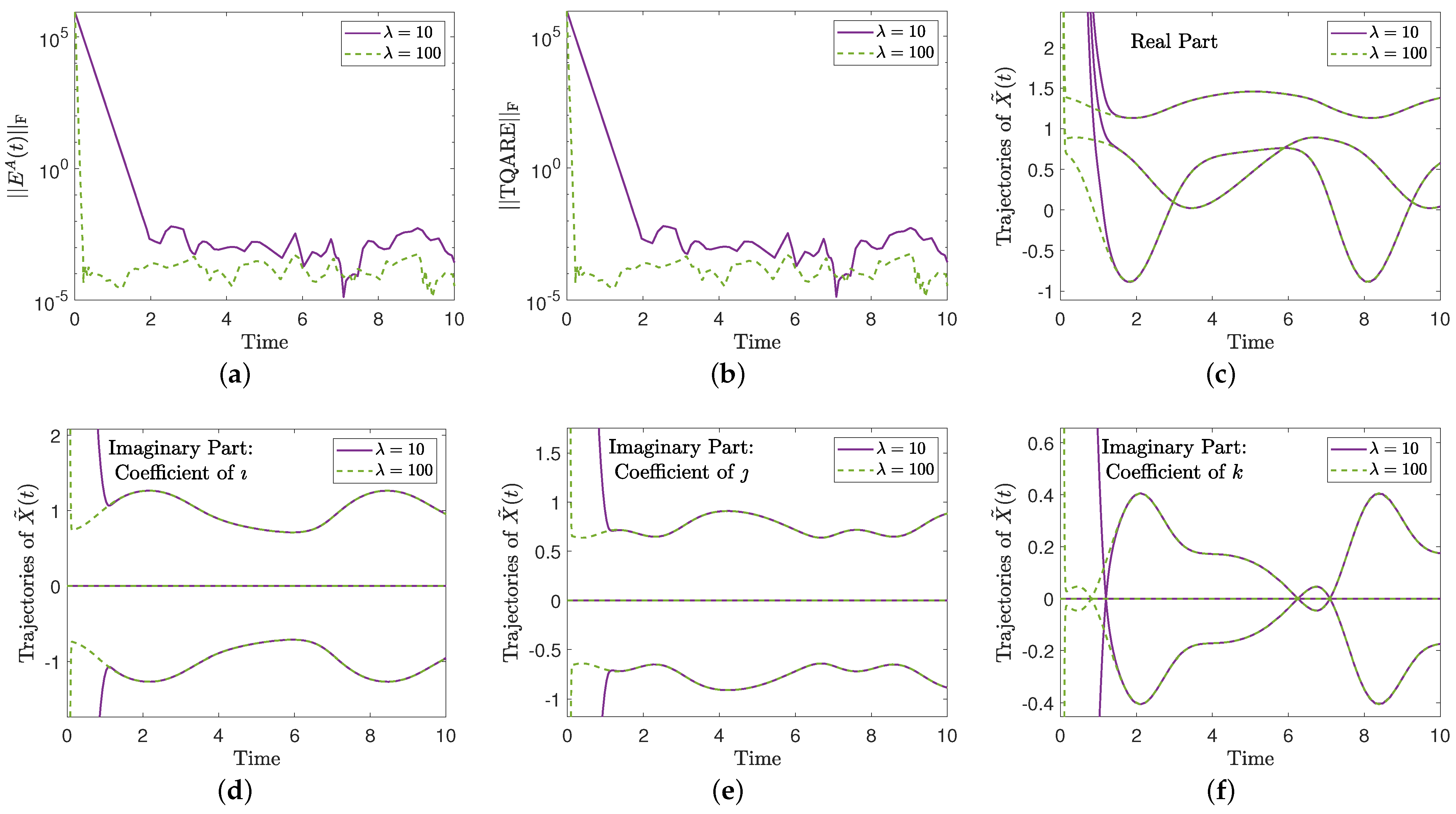
5.1.1. Example 1

The coefficients of matrix $\tilde{A}(t)$ in this SE are configured as follows:

$$\begin{array}{c}{A}_1(t)=\left[\begin{array}{cc}6\gamma (t)+1& 4\\ 5\eta (t)+2& 6\end{array}\right],A_2(t)=\left[\begin{array}{cc}0& 2\gamma (t)+2\\ 4\gamma (t)-2& 0\end{array}\right],\hfill \\ A_3(t)=\left[\begin{array}{cc}0& 5\\ 5\gamma (t)+1& 0\end{array}\right],A_4(t)=\left[\begin{array}{cc}0& 2\gamma (t)+3\\ 2& 0\end{array}\right].\hfill \end{array}$$

the coefficients of matrix $\tilde{B}(t)$ are configured as follows:

$$\begin{array}{c}{B}_1(t)=\left[\begin{array}{cc}\eta (t)& \gamma (t)+3\\ \gamma (t)+3& \gamma (t)+2\end{array}\right],B_2(t)=\left[\begin{array}{cc}0& 6\\ -6& 0\end{array}\right],\hfill \\ B_3(t)=\left[\begin{array}{cc}0& 5+\eta (t)\\ -5-\eta (t)& 0\end{array}\right],B_4(t)=\left[\begin{array}{cc}0& \eta (t)\\ -\eta (t)& 0\end{array}\right],\hfill \end{array}$$

and the coefficients of matrix $\tilde{C}(t)$ are configured as follows:

$$\begin{array}{c}{C}_1(t)=\left[\begin{array}{cc}\gamma (t)+5& \eta (t)\\ \eta (t)& \eta (t)+2\end{array}\right],C_2(t)=\left[\begin{array}{cc}0& 5+\gamma (t)\\ -5-\gamma (t)& 0\end{array}\right],\hfill \\ C_3(t)=\left[\begin{array}{cc}0& 6\\ -6& 0\end{array}\right],C_4(t)=\left[\begin{array}{cc}0& \gamma (t)\\ -\gamma (t)& 0\end{array}\right].\hfill \end{array}$$

Hence, $\tilde{A}(t),\tilde{B}(t),\tilde{C}(t)\in {\mathbb{H}}^{2\times 2}$. Additionally, the initial condition of the ZQ-ARE model has been set to $\mathbf{x}(0)=100\odot {\mathbf{1}}_6$, and the parameter $\lambda$ is employed with values of 10 and 100 in order to verify the convergence features of the ZNN technique. The ZQ-ARE model’s findings are depicted in Figure 1.

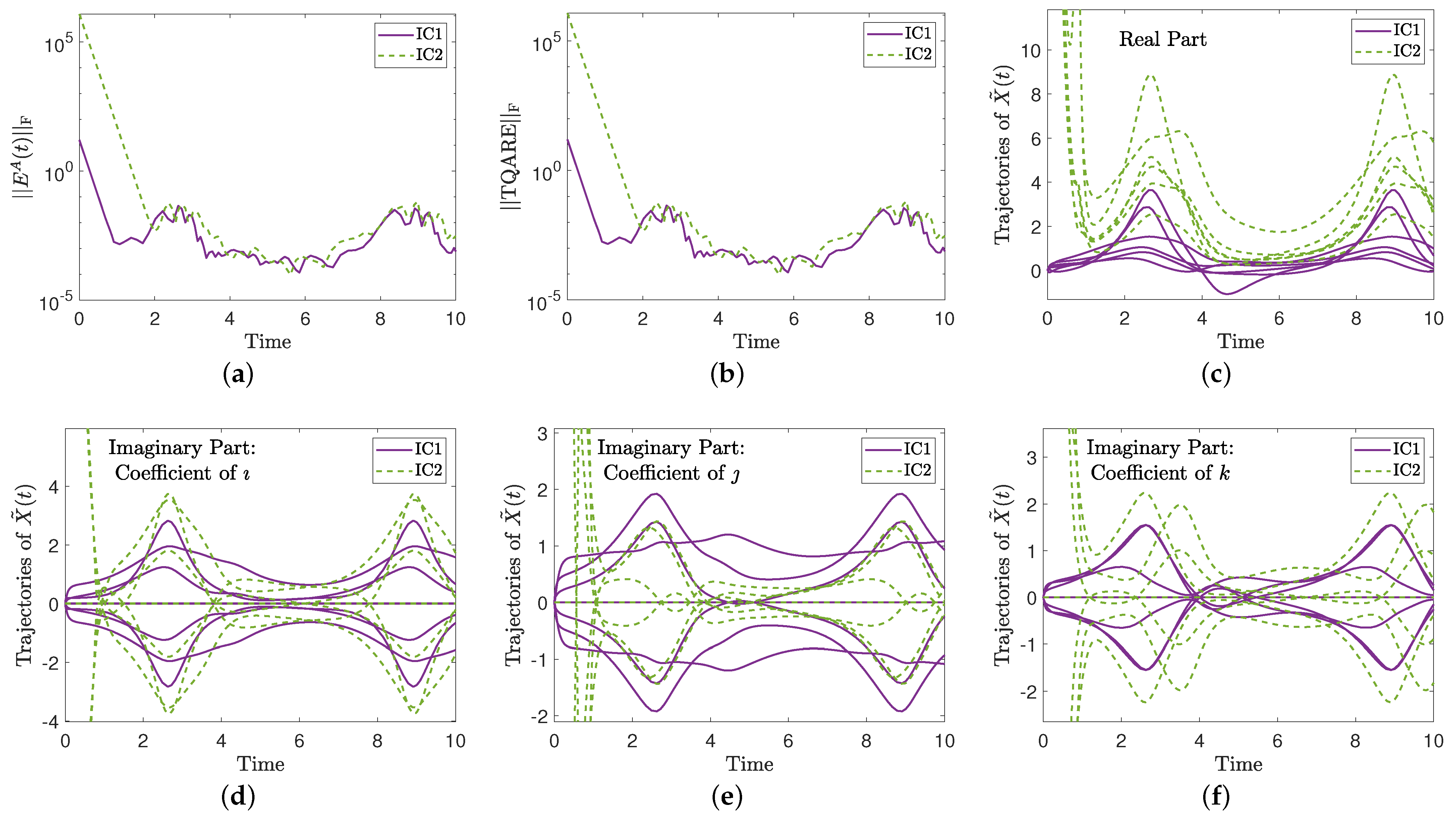
5.1.2. Example 2

Consider the following $3\times 3$ real matrices:

$$M_1=\left[\begin{array}{ccc}0& 0& 1\\ 0& 0& 0\\ -1& 0& 0\end{array}\right],M_2=\left[\begin{array}{ccc}0& 1& 0\\ -1& 0& 0\\ 0& 0& 0\end{array}\right],M_3=\left[\begin{array}{ccc}0& 0& 0\\ 0& 0& 1\\ 0& -1& 0\end{array}\right].$$

Then, the coefficients of matrix $\tilde{A}(t)$ in this SE are configured as follows:

$$\begin{array}{c}{A}_1(t)={\mathbf{1}}_{3\times 3}+I_3\odot \gamma (t),A_2(t)=M_1\odot (1+\gamma (t)),\hfill \\ A_3(t)=M_2\odot (2+2\gamma (t)),A_4(t)=M_3\odot (3+\gamma (t)),\hfill \end{array}$$

the coefficients of matrix $\tilde{B}(t)$ are configured as follows:

$$\begin{array}{c}{B}_1(t)=I_3\odot (1+\gamma (t)),B_2(t)=M_1\odot (4+2\eta (t)),\hfill \\ B_3(t)=M_2\odot (1+\eta (t)),B_4(t)=M_3\odot (3+2\eta (t)),\hfill \end{array}$$

and the coefficients of matrix $\tilde{C}(t)$ are configured as follows:

$$\begin{array}{c}{C}_1(t)=I_3\odot (1+\eta (t)),C_2(t)=M_1\odot (5+\eta (t)),\hfill \\ C_3(t)=M_2\odot (7+\eta (t)),C_4(t)=M_3\odot (1+3\eta (t)).\hfill \end{array}$$

Therefore, $\tilde{A}(t),\tilde{B}(t),\tilde{C}(t)\in {\mathbb{H}}^{3\times 3}$. Additionally, the parameter $\lambda$ of the ZQ-ARE model is utilized with a value of 10, and the initial conditions (ICs) are set as follows:

• IC1: $\mathbf{x}(0)={\mathbf{0}}_{15}$;
• IC2: $\mathbf{x}(0)=100\odot {\mathbf{1}}_{15}$.

Notice that we use two ICs in order to verify the results of Theorem 2. The ZQ-ARE model’s findings are depicted in Figure 2.

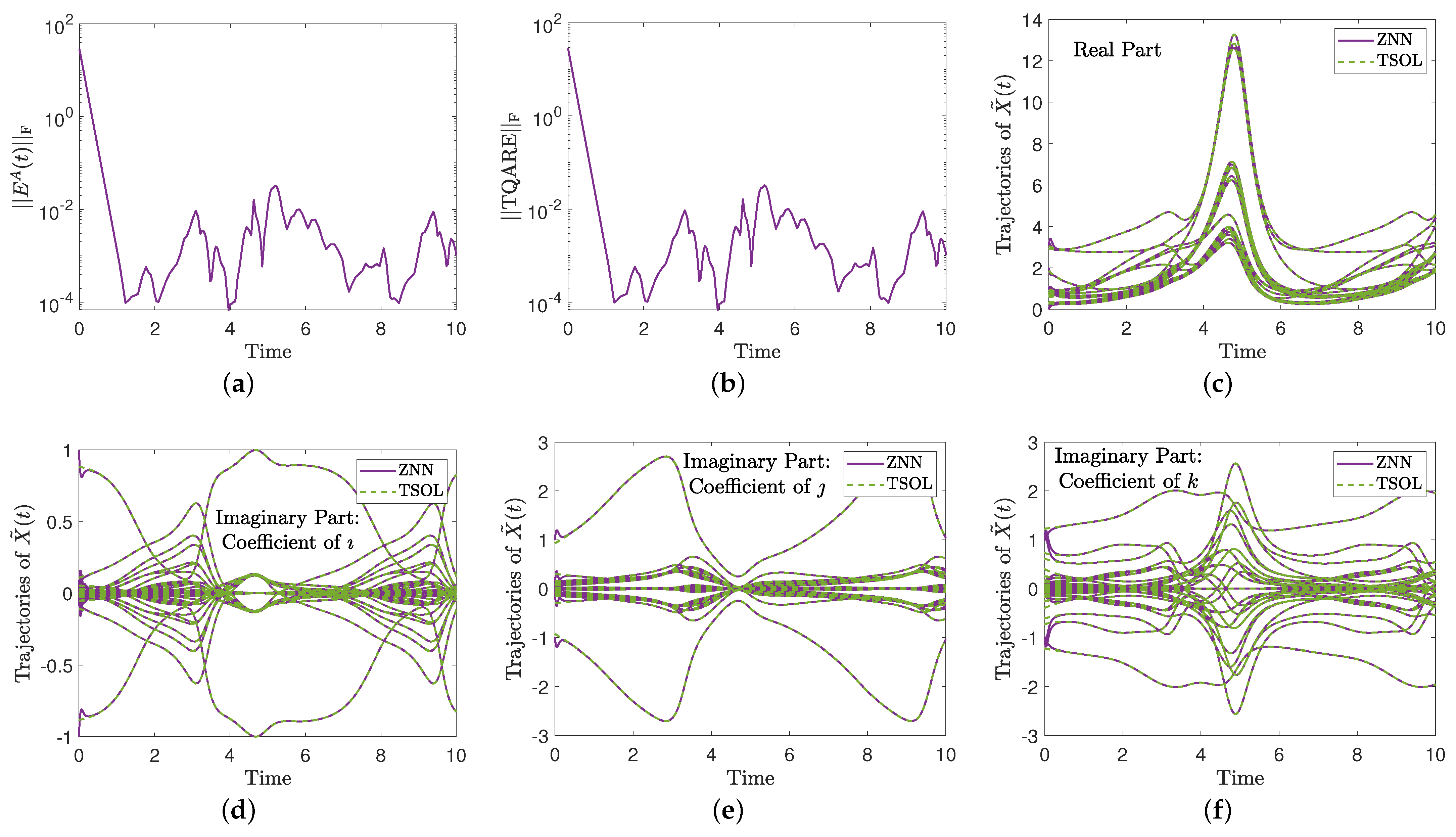
5.1.3. Example 3

Consider the following $6\times 6$ real matrices:

$$M_1=\left[\begin{array}{cccccc}0& 0& 0& 0& 0& 1\\ 0& 0& 0& 0& 0& 0\\ 0& 0& 0& 0& 0& 0\\ 0& 0& 0& 0& 0& 0\\ 0& 0& 0& 0& 0& 0\\ -1& 0& 0& 0& 0& 0\end{array}\right],M_2=\left[\begin{array}{cccccc}0& 0& 0& 1& 0& 0\\ 0& 0& 0& 0& 0& 0\\ 0& 0& 0& 0& 0& 0\\ -1& 0& 0& 0& 0& 0\\ 0& 0& 0& 0& 0& 0\\ 0& 0& 0& 0& 0& 0\end{array}\right],M_3=\left[\begin{array}{cccccc}0& 0& 0& 0& 0& 0\\ 0& 0& 1& 0& 0& 0\\ 0& -1& 0& 0& 0& 0\\ 0& 0& 0& 0& 0& 0\\ 0& 0& 0& 0& 0& 0\\ 0& 0& 0& 0& 0& 0\end{array}\right].$$

Then, the coefficients of matrix $\tilde{A}(t)$ in this SE are configured as follows:

$$\begin{array}{c}{A}_1(t)={\mathbf{1}}_{6\times 6}+I_6\odot \gamma (t),A_2(t)=M_1\odot (1+\gamma (t)),\hfill \\ A_3(t)=M_2\odot (2+2\gamma (t)),A_4(t)=M_3\odot (3+\gamma (t)),\hfill \end{array}$$

the coefficients of matrix $\tilde{B}(t)$ are configured as follows:

$$\begin{array}{c}{B}_1(t)=I_6\odot (1+\gamma (t)),B_2(t)=M_1\odot (4+2\eta (t)),\hfill \\ B_3(t)=M_2\odot (1+\eta (t)),B_4(t)=M_3\odot (3+2\eta (t)),\hfill \end{array}$$

and matrix $\tilde{C}(t)=\tilde{B}(t)$. Therefore, $\tilde{A}(t),\tilde{B}(t),\tilde{C}(t)\in {\mathbb{H}}^{6\times 6}$. Additionally, the parameter $\lambda$ of the ZQ-ARE model is utilized with a value of 10, and the initial condition is set as $\mathbf{x}(0)=\mathrm{round}({\mathbf{x}}_{\mathcal{T}\mathcal{S}}(0))$, where $\mathrm{round}(·)$ denotes an element-wise round function of all inputs, and ${\mathbf{x}}_{\mathcal{T}\mathcal{S}}$ is the eigenvector solution [48]. It is important to note that in order for the ZQ-ARE model to find a solution that matches a certain TSOL, we utilize an initial condition that is near that TSOL. The ZQ-ARE model’s findings are depicted in Figure 3.

5.2. Discussion of the SE Findings

Throughout Section 5.1.1–Section 5.1.3, the effectiveness of the ZQ-ARE (20) model for solving the TQARE of (2) is examined. Because of the appropriate matrices $\tilde{B}(t)$, $\tilde{C}(t)$, and $\tilde{A}(t)$, each SE has a distinct TQARE.

It can be seen that $\tilde{A}(t),\tilde{B}(t),\tilde{C}(t)\in {\mathbb{H}}^{2\times 2}$ in Section 5.1.1. In other words, $n=2$ in (2)’s TQARE. For $\lambda =10$ and $\lambda =100$, we have the following results for the ZQ-ARE model. Figure 1a illustrates the ZQ-ARE model’s EMEs. The two cases in this illustration begin with a big error value at $t=0$ and end up with a tiny error value in the interval $[{10}^{-5},{10}^{-3}]$ at $t=2$ when $\lambda =10$ and at $t=0.1$ when $\lambda =100$. Stated differently, the convergence features of the ZNN approach are verified by the EME of the ZQ-ARE model, which is influenced by the value of $\lambda$. The ZQ-ARE model’s (2) error is displayed in Figure 1b. The results displayed there confirm those in Figure 1a, indicating that solving (10) is the same as solving (2). The solutions produced by the model are shown as trajectories in Figure 1c–f. These figures display the real part and the three imaginary parts of the solutions, respectively. It is demonstrated that the models provide the same solutions and that their convergence to the TSOL is consistent with the related EMEs’ tendency towards convergence.

Furthermore, it can be seen that $\tilde{A}(t),\tilde{B}(t),\tilde{C}(t)\in {\mathbb{H}}^{3\times 3}$ in Section 5.1.2. In other words, $n=3$ in (2)’s TQARE. Under IC1 and IC2 for $\lambda =10$, we have the following results for the ZQ-ARE model. Figure 2a illustrates the ZQ-ARE model’s EMEs. The two cases in this illustration begin with a big error value at $t=0$: with IC2’s initial error value being substantially larger than IC1’s. However, the EMEs reach a tiny error value in the interval $[{10}^{-4},{10}^{-3}]$ at $t=1$ in the instance of IC1 and at $t=2$ in the instance of IC2. Stated differently, Theorem 2 is validated by the ZQ-ARE model, which converges to a low value for two distinctive ICs. The ZQ-ARE model’s (2) error is displayed in Figure 2b. The results displayed there confirm those in Figure 2a, indicating that solving (10) is the same as solving (2). The solutions produced by the model are shown as trajectories in Figure 2c–f. These figures display the real part and the three imaginary parts of the solutions, respectively. It is demonstrated that the models provide the same solutions and that their convergence to the TSOL is consistent with the related EMEs’ tendency towards convergence.

Additionally, it can be seen that $\tilde{A}(t),\tilde{B}(t),\tilde{C}(t)\in {\mathbb{H}}^{6\times 6}$ in Section 5.1.3. In other words, $n=6$ in (2)’s TQARE. Under an initial condition that is near to the eigenvector TSOL and for $\lambda =10$, we have the following results for the ZQ-ARE model. Figure 3a illustrates the ZQ-ARE model’s EME. The EME in this illustration begins with a big error value at $t=0$ and reaches a tiny error value in the interval $[{10}^{-4},{10}^{-2}]$ at $t=1$. The ZQ-ARE model’s (2) error is displayed in Figure 3b. The results displayed there confirm those in Figure 3a, indicating that solving (10) is the same as solving (2). The solutions produced by the model are shown as trajectories in Figure 3c–f. These figures display the real part and the three imaginary parts, respectively, of the ZQ-ARE model’s solution and the eigenvector TSOL. It is demonstrated that the model provides the same solution and that its convergence to the eigenvector TSOL is consistent with the related EME’s tendency towards convergence. Stated differently, Theorem 2 is validated by the ZQ-ARE model, which converges to the TSOL.

When everything is considered, the ZQ-ARE model solves three distinct TQAREs quite well. It is noteworthy that the discussion given above confirms the ZNN technique’s convergence qualities and Theorem 2’s findings. Additionally, the ZQ-ARE model’s computational complexity is $\mathcal{O}({(2n^2-n)}^3)$, which is similar to that of other ZNN models that approach various quaternion matrix equations (see [25,28,30,31,32]).

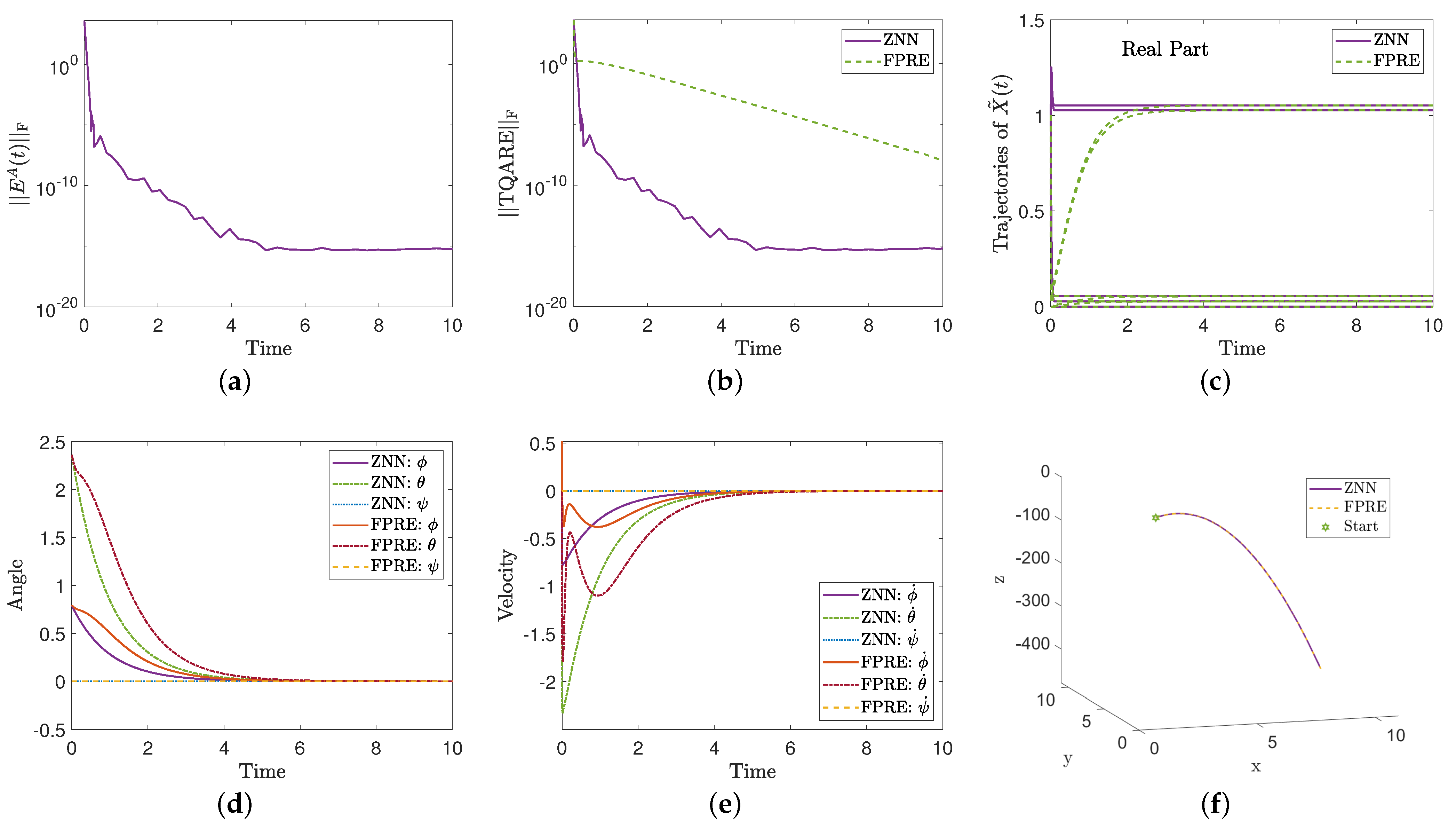
5.3. Application to Quadrotor Control

In this application, the ZNN design technique is used to stabilize the quadcopter device of Figure 4. Determining the position of a quadcopter requires the definition of coordinate systems since it is a vehicle with four separate drives and, at its center of gravity, an electric power system [49,50]. Three Euler angles and the vertical movement in the global coordinate system are the control parameters for a six-degree-of-freedom model device [51,52]. In order to ensure independent control over each drive and minimal aerodynamic effects, it is necessary to consider a fixed-frame body and a symmetrical model structure with the origin in the mass center [53,54].

Our approach uses the dynamic model derived from [55,56], which consists of the following equation system:

$$\left\{\begin{array}{c}\ddot{x}=\frac{u_1}{m}(\eta (\varphi )\gamma (\theta )\eta (\psi )+\gamma (\varphi )\gamma (\psi ))\hfill \\ \ddot{y}=\frac{u_1}{m}(\eta (\varphi )\gamma (\theta )\gamma (\psi )-\gamma (\varphi )\eta (\psi ))\hfill \\ \ddot{z}=\frac{u_1}{m}\eta (\varphi )\eta (\psi )-g\hfill \\ \ddot{\varphi }=\frac{{\mathcal{I}}_y-{\mathcal{I}}_z}{{\mathcal{I}}_x}\dot{\theta }\dot{\psi }-\frac{J_R}{{\mathcal{I}}_x}\dot{\theta }{\omega }_d+\frac{l}{{\mathcal{I}}_x}{u}_2\hfill \\ \ddot{\theta }=\frac{{\mathcal{I}}_z-{\mathcal{I}}_x}{{\mathcal{I}}_y}\dot{\varphi }\dot{\psi }-\frac{J_R}{{\mathcal{I}}_y}\dot{\varphi }{\omega }_d+\frac{l}{{\mathcal{I}}_y}{u}_3\hfill \\ \ddot{\psi }=\frac{{\mathcal{I}}_x-{\mathcal{I}}_y}{{\mathcal{I}}_z}\dot{\varphi }\dot{\theta }+\frac{l}{{\mathcal{I}}_z}{u}_4,\hfill \end{array}\right.$$

(29)

where the position of the quadrotor is described by the coordinates $x,y,z$ in the global coordinate system, and its orientation is described by the three Euler angles: i.e., the yaw angle $\psi \in [-\pi ,\pi ]$, pitch angle $\theta \in [-\pi /2,\pi /2]$, and roll angle $\varphi \in [-\pi ,\pi ]$. Additionally, g is the gravitational acceleration, l is the quadrotor’s arm length, d is the factor of drag, ${\omega }_d$ is the relative motor speed, ${\mathcal{I}}_x,{\mathcal{I}}_y,{\mathcal{I}}_z$ are inertias, $J_R$ is the rotor inertia, m is the quadrotor’s mass, and $u_j,j=1,\dots ,4$ are the input variables of the system.

The state-space formation of (29) is the following:

$$\dot{\mathbf{x}}=\left[\begin{array}{c}{x}_2\\ \frac{u_1}{m}(\eta (x_7)\gamma (x_9)\eta (x_{11})+\gamma (x_7)\gamma (x_{11}))\\ x_4\\ \frac{u_1}{m}(\eta (x_7)\gamma (x_9)\gamma (x_{11})+\gamma (x_7)\eta (x_{11}))\\ x_6\\ \frac{u_1}{m}\eta (x_7)\eta (x_9)-g\\ x_8\\ \frac{{\mathcal{I}}_y-{\mathcal{I}}_z}{{\mathcal{I}}_x}{x}_{12}{x}_{10}-\frac{J_R}{{\mathcal{I}}_x}{x}_{10}{\omega }_d+\frac{l}{{\mathcal{I}}_x}{u}_2\\ x_{10}\\ \frac{{\mathcal{I}}_z-{\mathcal{I}}_x}{{\mathcal{I}}_y}{x}_{12}{x}_8-\frac{J_R}{{\mathcal{I}}_y}{x}_8{\omega }_d+\frac{l}{{\mathcal{I}}_y}{u}_3\\ x_{12}\\ \frac{{\mathcal{I}}_x-{\mathcal{I}}_y}{{\mathcal{I}}_z}{x}_{10}{x}_8+\frac{l}{{\mathcal{I}}_z}{u}_4,\end{array}\right]$$

(30)

where $\mathbf{x}={\left[\begin{array}{c}x,\dot{x},y,\dot{y},z,\dot{z},\varphi ,\dot{\varphi },\theta ,\dot{\theta },\psi ,\dot{\psi }\end{array}\right]}^{\mathrm{T}}={\left[\begin{array}{c}{x}_1,x_2,\dots ,x_{12}\end{array}\right]}^{\mathrm{T}}\in {\mathbb{R}}^{12}$ is the state vector and $u={\left[\begin{array}{c}{u}_1,u_2,u_3,u_4\end{array}\right]}^{\mathrm{T}}\in {\mathbb{R}}^4$ is the control vector.

In order to solve an ARE and derive the suboptimal control rule, it is crucial to note that the SDRE control approach reconstructs the nonlinear dynamics utilizing parameterization into a linear form with coefficient state-dependent matrices [57]. In the state space, the ARE equation’s coefficients vary. Therefore, it is necessary to solve a state-dependent ARE at any point in the state space. We are able to get more degrees of freedom because the state-dependent parameterization is nonunique, which can potentially improve controller performance. The structure is similar to that of a quadratic when the nonlinear performance index is minimized.

Consider the optimal control issue for the next linear time-varying system [58]:

$$\dot{\mathbf{x}}(t)=A(t)\mathbf{x}(t)+L(t)u(t),$$

(31)

where $\mathbf{x}(t)\in {\mathbb{R}}^n$, $L(t)\in {\mathbb{R}}^{n\times m}$, $A(t)\in {\mathbb{R}}^{n\times n}$, and $u(t)\in {\mathbb{R}}^m$. Control gains at any state $\mathbf{x}(t)$ can be calculated using standard linear optimal control theory, i.e., choosing the control that minimizes the following cost function:

$$J=0.5{\int }_0^{\infty }{\mathbf{x}}^{\mathrm{T}}(t)C(t)\mathbf{x}(t)+u^{\mathrm{T}}(t)G(t)u(t)\mathrm{d}t,$$

(32)

where $C(t)\in {\mathbb{R}}^{n\times n}$ penalizes the state and $G(t)\in {\mathbb{R}}^{m\times m}$ penalizes the control effort. By obtaining $X(t)$, which is the solution to the next continuous-time ARE (CARE):

$$X(t)A(t)+A^{\mathrm{T}}(t)X(t)-X(t)L(t)G^{-1}(t)L^{\mathrm{T}}(t)X(t)+C(t)={\mathbf{0}}_{n\times n},$$

(33)

the control gains that minimizes (32) become:

$$u(t)=-G^{-1}(t)L^{\mathrm{T}}(t)X(t)\mathbf{x}(t).$$

(34)

This controller’s stability features are verified in [59,60].

One traditional approach for solving (33) is to use the forward-propagating Riccati equation (FPRE) method [61]. Particularly, the solution of (33) is obtained through the following DARE:

$$\dot{X}(t)=X(t)A(t)+A^{\mathrm{T}}(t)X(t)-X(t)L(t)G^{-1}(t)L^{\mathrm{T}}(t)X(t)+C(t).$$

(35)

On the other hand, one different approach for solving (33) is to use the ZNN method as proposed in [62]. Particularly, by using $B(t)=L(t)G^{-1}(t)L^{\mathrm{T}}(t)$, it is readily understood that (33) may be turned into (2). As a result, the solution of (33) can be obtained through (20).

In our approach, the SDRE method is applied to the attitude control problem. The vector of the state variables for that problem is ${\mathbf{x}}_{\mathcal{I}}={\left[\begin{array}{c}{x}_7,x_8,\dots ,x_{12}\end{array}\right]}^{\mathrm{T}}\in {\mathbb{R}}^6$, and the vector of the input variables is $u_{\mathcal{I}}={\left[\begin{array}{c}{u}_2,u_3,u_4\end{array}\right]}^{\mathrm{T}}\in {\mathbb{R}}^3$, while the state-dependent model derived from (30) after factorization is the following:

$${\dot{\mathbf{x}}}_{\mathcal{I}}=\left[\begin{array}{cccccc}0& 1& 0& 0& 0& 0\\ 0& 0& 0& \frac{{\mathcal{I}}_y-{\mathcal{I}}_z}{{\mathcal{I}}_x}{x}_{12}& 0& 0\\ 0& 0& 0& 1& 0& 0\\ 0& \frac{{\mathcal{I}}_z-{\mathcal{I}}_x}{{\mathcal{I}}_y}{x}_{12}& 0& 0& 0& 0\\ 0& 0& 0& 0& 0& 1\\ 0& 0& 0& \frac{{\mathcal{I}}_x-{\mathcal{I}}_y}{{\mathcal{I}}_z}{x}_8& 0& 0\end{array}\right]·{\mathbf{x}}_{\mathcal{I}}+\left[\begin{array}{ccc}0& 0& 0\\ \frac{l}{{\mathcal{I}}_x}& 0& 0\\ 0& 0& 0\\ 0& \frac{l}{{\mathcal{I}}_y}& 0\\ 0& 0& 0\\ 0& 0& \frac{l}{{\mathcal{I}}_z}\end{array}\right]·u_{\mathcal{I}},$$

(36)

where $A(t)\in {\mathbb{R}}^{6\times 6}$ and $L(t)\in {\mathbb{R}}^{6\times 3}$. Thereafter, we set $\tilde{A}(t)=A(t)$, $\tilde{C}(t)=G(t)=I_6$, and $\tilde{B}(t)=L(t)G^{-1}(t)L^{\mathrm{T}}(t)$, and we use the parameter values of the object presented in

Table 1. The parameters utilized in the quadrotor simulation.

Parameter	Value	Unit
m	0.5	kg
g	9.81	m/s${}^2$
l	0.3	m
$J_R$	0.01	N
${\mathcal{I}}_x$	0.0081	kg·m${}^2$
${\mathcal{I}}_y$	0.0081	kg·m${}^2$
${\mathcal{I}}_z$	0.0162	kg·m${}^2$

and the ICs ${\mathbf{x}}_{\mathcal{I}}(0)={\left[\begin{array}{c}\pi /4,\pi /2,3\pi /4,0,0,0\end{array}\right]}^{\mathrm{T}}$. Additionally, the $\lambda$ parameter value is set to 100, and the ICs of the ZQ-ARE model and DARE have been set as follows:

$$\tilde{X}(0)=X(0)=\left[\begin{array}{ccc}{\mathbf{1}}_{2\times 2}& {\mathbf{0}}_{2\times 2}& {\mathbf{0}}_{2\times 2}\\ {\mathbf{0}}_{2\times 2}& {\mathbf{1}}_{2\times 2}& {\mathbf{0}}_{2\times 2}\\ {\mathbf{0}}_{2\times 2}& {\mathbf{0}}_{2\times 2}& {\mathbf{1}}_{2\times 2}\end{array}\right].$$

(37)

The results of the ZNN and FPRE methods are presented in Figure 5. Notice that the purpose of the control procedure is stabilization at the zero point.

Particularly, it can be seen that $\tilde{A}(t),\tilde{B}(t),\tilde{C}(t)\in {\mathbb{H}}^{6\times 6}$. In other words, $n=6$ in (2)’s TQARE. For $\lambda =100$, we have the following results for the ZQ-ARE model. Figure 5a illustrates the ZQ-ARE model’s EMEs. The EME in this image starts with a big value at $t=0$ and ends up with a small value in the interval $[{10}^{-16},{10}^{-15}]$ at $t=5$. Figure 5b depicts the (2) error of the ZQ-ARE solution of the ZNN method and the DARE solution of the FPRE method. The findings show that the ZQ-ARE solution is more accurate than the DARE solution. Figure 5c displays the trajectories of the real parts of the solutions generated by the models; the solutions’ imaginary parts are left out because they are zeros. This graph shows that although the models produce identical solutions, the ZNN approach converges more quickly than the FPRE method. Figure 5d shows the time-plot of the quadrotor’s angles, and Figure 5e shows the time-plot of the quadrotor’s velocities. These graphs demonstrate that stabilization at the “zero” point for the angles and velocities is successful by both models, but the ZNN method achieve faster stabilization than the FPRE method. Figure 5f shows the quadrotor’s position during attitude control, where we can observe that the ZNN and FPRE methods produce identical results. Based on the aforementioned observations, the results of the application to quadrotor control show that the ZNN method is more effective than the FPRE method. To conclude, the ZNN method is not only fruitful for solving the TQARE, but it may also be employed to quadrotor control with high efficiency.

6. Conclusions

In this paper, a novel ZNN model, termed ’ZQ-ARE’, is presented for solving the TQARE by identifying only Hermitian solutions. Theoretical investigation and simulation experiments are conducted to support the ZQ-ARE model’s accuracy and efficiency, while an application to quadrotor control is carried out to support the ZQ-ARE model’s practical applicability. Specifically, in three SEs, the ZQ-ARE model finds the TQARE Hermitian solutions under various initial conditions, and we also demonstrate that the convergence rate of the solution increases as the value of the parameter $\lambda$ rises.For the purpose of stabilizing the flight control system of a quadrotor, a comparison is given between the solution adaptations provided by the ZNN and FPRE methods. The results of this application show that the ZNN method is more effective than the FPRE method. So we can conclude that the ZNN method is not only fruitful for solving the TQARE, but it may also be employed for quadrotor control with high efficiency.

It is significant to mention that the suggested ZNN model has the drawback of being noise-intolerant since all kinds of noise significantly affect the suggested ZNN approach’s accuracy. Therefore, the adaptation of this model to a noise-tolerant ZNN design could be the main focus of future study. To be more precise, the suggested model might be made noise-tolerant by substituting the original ZNN design with a noise-tolerant ZNN architecture, such as the one used in [37]. Moreover, future research may involve applying the proposed ZNN model to a range of other technical issues, including secure communications with application to acoustic source tracking [63] and network and power systems with application to chaotic system stabilization [64,65].

References

- Kalman, R.E. Contributions to the theory of optimal control. Bol. Soc. Mat. Mex. 1960, 5, 102–119. [Google Scholar]
- Qin, B.; Sun, H.; Ma, J.; Li, W.; Ding, T.; Wang, Z.; Zomaya, A.Y. Robust H∞ control of doubly fed wind generator via state-dependent Riccati equation technique. IEEE Trans. Power Syst. 2019, 34, 2390–2400. [Google Scholar] [CrossRef]
- Dong, X.; Hu, G. Time-varying formation tracking for linear multiagent systems with multiple leaders. IEEE Trans. Autom. Control 2017, 62, 3658–3664. [Google Scholar] [CrossRef]
- Rigatos, G.; Busawon, K.; Pomares, J.; Abbaszadeh, M. Nonlinear optimal control for the wheeled inverted pendulum system. Robotica 2020, 38, 29–47. [Google Scholar] [CrossRef]
- Laub, A. A Schur method for solving algebraic Riccati equations. IEEE Trans. Autom. Control. 1979, 24, 913–921. [Google Scholar] [CrossRef]
- Aguilar, L.T.; Orlov, Y.; Acho, L. Nonlinear H∞-control of nonsmooth time-varying systems with application to friction mechanical manipulators. Automatica 2003, 39, 1531–1542. [Google Scholar] [CrossRef]
- Mohammadi, H.; Zare, A.; Soltanolkotabi, M.; Jovanović, M.R. Convergence and sample complexity of gradient methods for the model-free linear-quadratic regulator problem. IEEE Trans. Autom. Control. 2022, 67, 2435–2450. [Google Scholar] [CrossRef]
- Hambly, B.; Xu, R.; Yang, H. Policy gradient methods for the noisy linear quadratic regulator over a finite horizon. SIAM J. Control Optim. 2021, 59, 3359–3391. [Google Scholar] [CrossRef]
- Hossain, M.; Haque, M.E.; Arif, M.T. Kalman filtering techniques for the online model parameters and state of charge estimation of the Li-ion batteries: A comparative analysis. J. Energy Storage 2022, 51, 104174. [Google Scholar] [CrossRef]
- Hamidi, F.; Jerbi, H.; Alharbi, H.; Leiva, V.; Popescu, D.; Rajhi, W. Metaheuristic solution for stability analysis of nonlinear systems using an intelligent algorithm with potential applications. Fractal Fract. 2023, 7, 78. [Google Scholar] [CrossRef]
- Kchaou, M.; Regaieg, M.A.; Jerbi, H.; Abbassi, R.; Stefanoiu, D.; Popescu, D. Admissible control for non-linear singular systems subject to time-varying delay and actuator saturation: An interval type-2 fuzzy approach. Actuators 2023, 12, 30. [Google Scholar] [CrossRef]
- Oshman, Y.; Bar-Itzhack, I. Eigenfactor solution of the matrix Riccati equation—A continuous square root algorithm. IEEE Trans. Autom. Control. 1985, 30, 971–978. [Google Scholar] [CrossRef]
- Dooren, P.V. A generalized eigenvalue approach for solving Riccati equations. SIAM J. Sci. Stat. Comput. 1981, 2, 121–135. [Google Scholar] [CrossRef]
- Zhang, F. Quaternions and matrices of quaternions. Linear Algebra Its Appl. 1997, 251, 21–57. [Google Scholar] [CrossRef]
- Rodman, L. Topics in Quaternion Linear Algebra; Princeton Series in Applied Mathematics; Princeton University Press: Princeton, NJ, USA, 2014. [Google Scholar] [CrossRef]
- Hamilton, W.R. On a new species of imaginary quantities, connected with the theory of quaternions. Proc. R. Ir. Acad. 1840, 2, 424–434. [Google Scholar]
- Joldeş, M.; Muller, J.M. Algorithms for manipulating quaternions in floating-point arithmetic. In Proceedings of the 2020 IEEE 27th Symposium on Computer Arithmetic (ARITH), Portland, OR, USA, 7–10 June 2020; pp. 48–55. [Google Scholar]
- Szynal-Liana, A.; Włoch, I. Generalized commutative quaternions of the Fibonacci type. Bol. Soc. Mat. Mex. 2022, 28, 1. [Google Scholar] [CrossRef]
- Pavllo, D.; Feichtenhofer, C.; Auli, M.; Grangier, D. Modeling human motion with quaternion-based neural networks. Int. J. Comput. Vis. 2020, 128, 855–872. [Google Scholar] [CrossRef]
- Giardino, S. Quaternionic quantum mechanics in real Hilbert space. J. Geom. Phys. 2020, 158, 103956. [Google Scholar] [CrossRef]
- Goodyear, A.M.S.; Singla, P.; Spencer, D.B. Analytical state transition matrix for dual-quaternions for spacecraft pose estimation. In Proceedings of the AAS/AIAA Astrodynamics Specialist Conference, Maui, HI, USA, 13–17 January 2019; Univelt Inc.: Escondido, CA, USA, 2020; pp. 393–411. [Google Scholar]
- Kansu, M.E. Quaternionic representation of electromagnetism for material media. Int. J. Geom. Methods Mod. Phys. 2019, 16, 1950105. [Google Scholar] [CrossRef]
- Özgür, E.; Mezouar, Y. Kinematic modeling and control of a robot arm using unit dual quaternions. Robot. Auton. Syst. 2016, 77, 66–73. [Google Scholar] [CrossRef]
- Xiao, L.; Zhang, Y.; Huang, W.; Jia, L.; Gao, X. A dynamic parameter noise-tolerant zeroing neural network for time-varying quaternion matrix equation with applications. IEEE Trans. Neural Netw. Learn. Syst. 2022, 1–10. [Google Scholar] [CrossRef]
- Kovalnogov, V.N.; Fedorov, R.V.; Demidov, D.A.; Malyoshina, M.A.; Simos, T.E.; Mourtas, S.D.; Katsikis, V.N. Computing quaternion matrix pseudoinverse with zeroing neural networks. AIMS Math. 2023, 8, 22875–22895. [Google Scholar] [CrossRef]
- Xiao, L.; Cao, P.; Song, W.; Luo, L.; Tang, W. A fixed-time noise-tolerance ZNN model for time-variant inequality-constrained quaternion matrix least-squares problem. IEEE Trans. Neural Netw. Learn. Syst. 2023, 1–10. [Google Scholar] [CrossRef]
- Xiao, L.; Liu, S.; Wang, X.; He, Y.; Jia, L.; Xu, Y. Zeroing neural networks for dynamic quaternion-valued matrix inversion. IEEE Trans. Ind. Inform. 2022, 18, 1562–1571. [Google Scholar] [CrossRef]
- Aoun, S.B.; Derbel, N.; Jerbi, H.; Simos, T.E.; Mourtas, S.D.; Katsikis, V.N. A quaternion Sylvester equation solver through noise-resilient zeroing neural networks with application to control the SFM chaotic system. AIMS Math. 2023, 8, 27376–27395. [Google Scholar] [CrossRef]
- Tan, N.; Yu, P.; Ni, F. New varying-parameter recursive neural networks for model-free kinematic control of redundant manipulators with limited measurements. IEEE Trans. Instrum. Meas. 2022, 71, 1–14. [Google Scholar] [CrossRef]
- Abbassi, R.; Jerbi, H.; Kchaou, M.; Simos, T.E.; Mourtas, S.D.; Katsikis, V.N. Towards higher-order zeroing neural networks for calculating quaternion matrix inverse with application to robotic motion tracking. Mathematics 2023, 11, 2756. [Google Scholar] [CrossRef]
- Kovalnogov, V.N.; Fedorov, R.V.; Demidov, D.A.; Malyoshina, M.A.; Simos, T.E.; Katsikis, V.N.; Mourtas, S.D.; Sahas, R.D. Zeroing neural networks for computing quaternion linear matrix equation with application to color restoration of images. AIMS Math. 2023, 8, 14321–14339. [Google Scholar] [CrossRef]
- Kovalnogov, V.N.; Fedorov, R.V.; Shepelev, I.I.; Sherkunov, V.V.; Simos, T.E.; Mourtas, S.D.; Katsikis, V.N. A novel quaternion linear matrix equation solver through zeroing neural networks with applications to acoustic source tracking. AIMS Math. 2023, 8, 25966–25989. [Google Scholar] [CrossRef]
- Zhang, Y.; Ge, S.S. Design and analysis of a general recurrent neural network model for time-varying matrix inversion. IEEE Trans. Neural Netw. 2005, 16, 1477–1490. [Google Scholar] [CrossRef]
- Chai, Y.; Li, H.; Qiao, D.; Qin, S.; Feng, J. A neural network for Moore-Penrose inverse of time-varying complex-valued matrices. Int. J. Comput. Intell. Syst. 2020, 13, 663–671. [Google Scholar] [CrossRef]
- Wu, W.; Zheng, B. Improved recurrent neural networks for solving Moore-Penrose inverse of real-time full-rank matrix. Neurocomputing 2020, 418, 221–231. [Google Scholar] [CrossRef]
- Jiang, W.; Lin, C.L.; Katsikis, V.N.; Mourtas, S.D.; Stanimirović, P.S.; Simos, T.E. Zeroing neural network approaches based on direct and indirect methods for solving the Yang–Baxter-like matrix equation. Mathematics 2022, 10, 1950. [Google Scholar] [CrossRef]
- Jerbi, H.; Alharbi, H.; Omri, M.; Ladhar, L.; Simos, T.E.; Mourtas, S.D.; Katsikis, V.N. Towards higher-order zeroing neural network dynamics for solving time-varying algebraic Riccati equations. Mathematics 2022, 10, 4490. [Google Scholar] [CrossRef]
- Katsikis, V.N.; Stanimirović, P.S.; Mourtas, S.D.; Xiao, L.; Karabasević, D.; Stanujkić, D. Zeroing neural network with fuzzy parameter for computing pseudoinverse of arbitrary matrix. IEEE Trans. Fuzzy Syst. 2022, 30, 3426–3435. [Google Scholar] [CrossRef]
- Alharbi, H.; Jerbi, H.; Kchaou, M.; Abbassi, R.; Simos, T.E.; Mourtas, S.D.; Katsikis, V.N. Time-varying pseudoinversion based on full-rank decomposition and zeroing neural networks. Mathematics 2023, 11, 600. [Google Scholar] [CrossRef]
- Mourtas, S.D.; Katsikis, V.N. Exploiting the Black-Litterman framework through error-correction neural networks. Neurocomputing 2022, 498, 43–58. [Google Scholar] [CrossRef]
- Kovalnogov, V.N.; Fedorov, R.V.; Generalov, D.A.; Chukalin, A.V.; Katsikis, V.N.; Mourtas, S.D.; Simos, T.E. Portfolio insurance through error-correction neural networks. Mathematics 2022, 10, 3335. [Google Scholar] [CrossRef]
- Mourtas, S.D.; Kasimis, C. Exploiting mean-variance portfolio optimization problems through zeroing neural networks. Mathematics 2022, 10, 3079. [Google Scholar] [CrossRef]
- Qiao, S.; Wei, Y.; Zhang, X. Computing time-varying ML-weighted pseudoinverse by the Zhang neural networks. Numer. Funct. Anal. Optim. 2020, 41, 1672–1693. [Google Scholar] [CrossRef]
- Wang, X.; Stanimirovic, P.S.; Wei, Y. Complex ZFs for computing time-varying complex outer inverses. Neurocomputing 2018, 275, 983–1001. [Google Scholar] [CrossRef]
- Dai, J.; Tan, P.; Yang, X.; Xiao, L.; Jia, L.; He, Y. A fuzzy adaptive zeroing neural network with superior finite-time convergence for solving time-variant linear matrix equations. Knowl.-Based Syst. 2022, 242, 108405. [Google Scholar] [CrossRef]
- Groß, J.; Trenkler, G.; Troschke, S.O. Quaternions: Further contributions to a matrix oriented approach. Linear Algebra Its Appl. 2001, 326, 205–213. [Google Scholar] [CrossRef]
- Gupta, A.K. Numerical Methods Using MATLAB; MATLAB Solutions Series; Apress: Berkeley, CA, USA; New York, NY, USA, 2014. [Google Scholar]
- Simos, T.E.; Katsikis, V.N.; Mourtas, S.D.; Stanimirović, P.S. Unique non-negative definite solution of the time-varying algebraic Riccati equations with applications to stabilization of LTV systems. Math. Comput. Simul. 2022, 202, 164–180. [Google Scholar] [CrossRef]
- Carino, J.; Abaunza, H.; Castillo, P. Quadrotor quaternion control. In Proceedings of the 2015 International Conference on Unmanned Aircraft Systems (ICUAS), Denver, CO, USA, 9–12 June 2015; IEEE: Denver, CO, USA, 2015. [Google Scholar] [CrossRef]
- Fresk, E.; Nikolakopoulos, G. Experimental evaluation of a full quaternion based attitude quadrotor controller. In Proceedings of the 2015 IEEE 20th Conference on Emerging Technologies & Factory Automation (ETFA), Luxembourg, 8–11 September 2015; IEEE: Luxembourg, 2015. [Google Scholar] [CrossRef]
- Chen, Y.; Perez-Arancibia, N.O. Adaptive control of aerobatic quadrotor maneuvers in the presence of propeller-aerodynamic-coefficient and torque-latency time-variations. In Proceedings of the 2019 International Conference on Robotics and Automation (ICRA), Montreal, QC, Canada, 20–24 May 2019; IEEE: Montreal, QC, Canada, 2019. [Google Scholar] [CrossRef]
- Nekoo, S.R.; Acosta, J.Á.; Ollero, A. Quaternion-based state-dependent differential Riccati equation for quadrotor drones: Regulation control problem in aerobatic flight. Robotica 2022, 40, 3120–3135. [Google Scholar] [CrossRef]
- Liang, T.; Yang, K.; Han, Q.; Li, C.; Li, J.; Deng, Q.; Chen, S.; Tuo, X. Attitude estimation of quadrotor UAV based on QUKF. IEEE Access 2023, 11, 111133–111141. [Google Scholar] [CrossRef]
- Li, J.; Chen, P.; Chang, Z.; Zhang, G.; Guo, L.; Zhao, C. Trajectory tracking control of quadrotor based on fractional-order s-plane model. Machines 2023, 11, 672. [Google Scholar] [CrossRef]
- Stepień, S.; Superczyńska, P. Modified infinite-time state-dependent Riccati equation method for nonlinear affine systems: Quadrotor control. Appl. Sci. 2021, 11, 10714. [Google Scholar] [CrossRef]
- Voos, H. Nonlinear state-dependent Riccati equation control of a quadrotor UAV. In Proceedings of the 2006 IEEE Conference on Computer Aided Control System Design, 2006 IEEE International Conference on Control Applications, 2006 IEEE International Symposium on Intelligent Control, Munich, Germany, 4–6 October 2006; IEEE: Munich, Germany, 2006. [Google Scholar] [CrossRef]
- Tan, S.; Zhong, W. Numerical solutions of linear quadratic control for time-varying systems via symplectic conservative perturbation. Appl. Math. Mech. 2007, 28, 277–287. [Google Scholar] [CrossRef]
- Weiss, A.; Kolmanovsky, I.; Bernstein, D.S. Forward-integration Riccati-based output-feedback control of linear time-varying systems. In Proceedings of the 2012 American Control Conference (ACC), Montreal, QC, Canada, 27–29 June 2012; pp. 6708–6714. [Google Scholar]
- Mracek, C.P.; Cloutier, J.R. Control designs for the nonlinear benchmark problem via the state-dependent Riccati equation method. Int. J. Robust Nonlinear Control 1998, 8, 401–433. [Google Scholar] [CrossRef]
- Erdem, E.B.; Alleyne, A.G. Design of a class of nonlinear controllers via state dependent Riccati equations. IEEE Trans. Control. Syst. Technol. 2004, 12, 133–137. [Google Scholar] [CrossRef]
- Prach, A.; Tekinalp, O.; Bernstein, D.S. A numerical comparison of frozen-time and forward-propagating Riccati equations for stabilization of periodically time-varying systems. In Proceedings of the American Control Conference, Portland, OR, USA, 4–6 June 2014; pp. 5633–5638. [Google Scholar]
- Simos, T.E.; Katsikis, V.N.; Mourtas, S.D.; Stanimirović, P.S. Solving time-varying nonsymmetric algebraic Riccati equations with zeroing neural dynamics. IEEE Trans. Syst. Man Cybern. Syst. 2023, 53, 6575–6587. [Google Scholar] [CrossRef]
- He, W.; Luo, T.; Tang, Y.; Du, W.; Tian, Y.; Qian, F. Secure communication based on quantized synchronization of chaotic neural networks under an event-triggered strategy. IEEE Trans. Neural Netw. Learn. Syst. 2020, 31, 3334–3345. [Google Scholar] [CrossRef] [PubMed]
- Su, H.; Luo, R.; Huang, M.; Fu, J. Robust fixed time control of a class of chaotic systems with bounded uncertainties and disturbances. Int. J. Control Autom. Syst. 2022, 20, 813–822. [Google Scholar] [CrossRef]
- Singer, J.; Wang, Y.; Bau, H.H. Controlling a chaotic system. Phys. Rev. Lett. 1991, 66, 1123. [Google Scholar] [CrossRef]