
Dynamic Analysis of the EU Countries Sustainability: Methods, Models, and Case Study


Abstract
:1. Introduction
2. Literature Review/Background
- Group I: Low resistance and slow recovery ().
- Group II: Low resistance and fast recovery ().
- Group III: High resistance and slow recovery ().
- Group IV: High resistance and fast recovery ().
- (1)
- Arithmetic mean index—the average of six regional development performance indicators: economic growth rate (EGR), open unemployment rate (UNP), poverty rate (POV), human development index (HDI), Gini index (GI), and environmental quality index (IKLH);
- (2)
- Geometric mean index ():
- (3)
- Entropic index ():
3. Materials and Methods
4. Main Part/Results
4.1. A Visual Representation of the Level of Absolute Instability of Development of the EU Countries in the Context of Individual Indicators
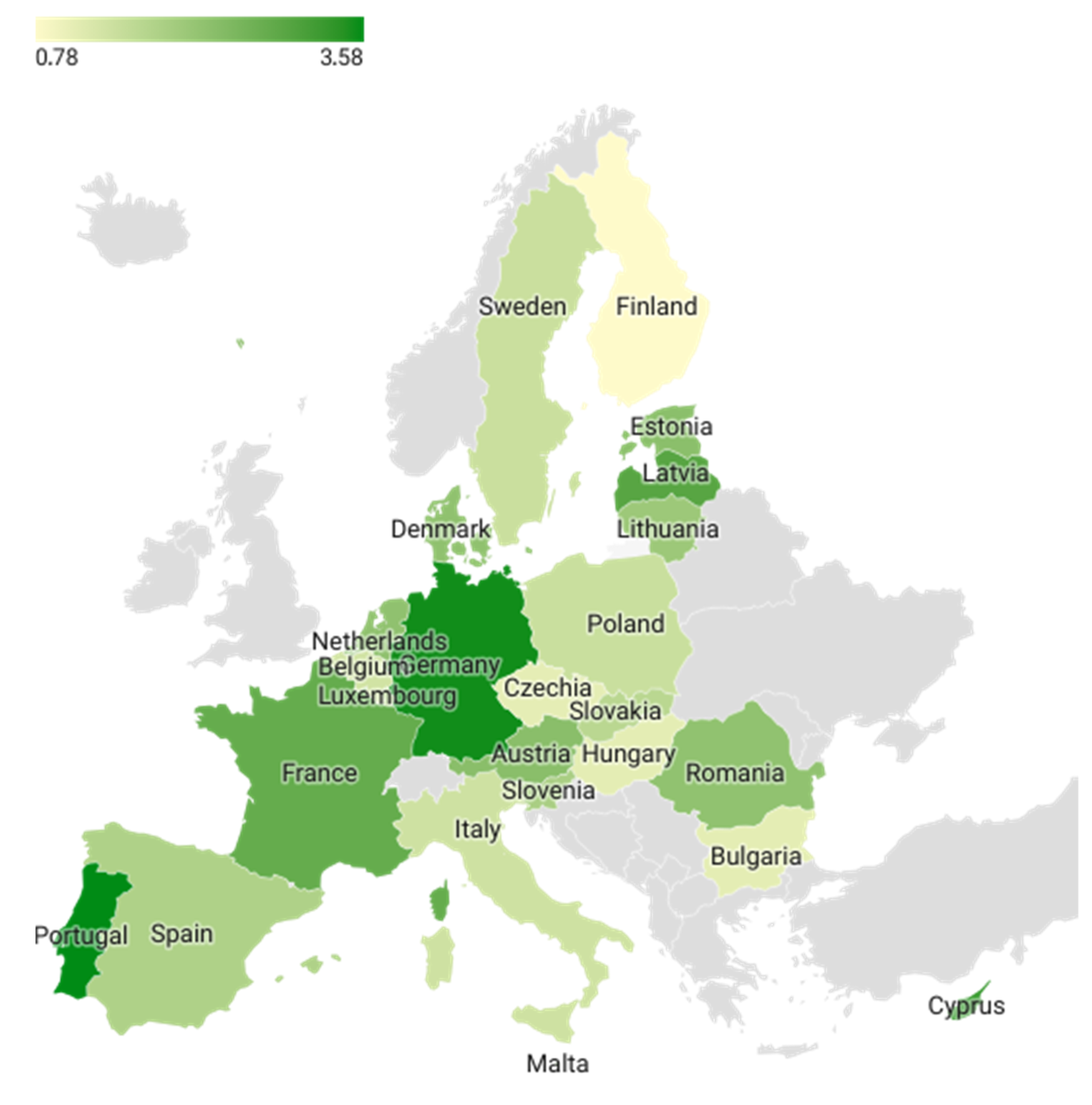
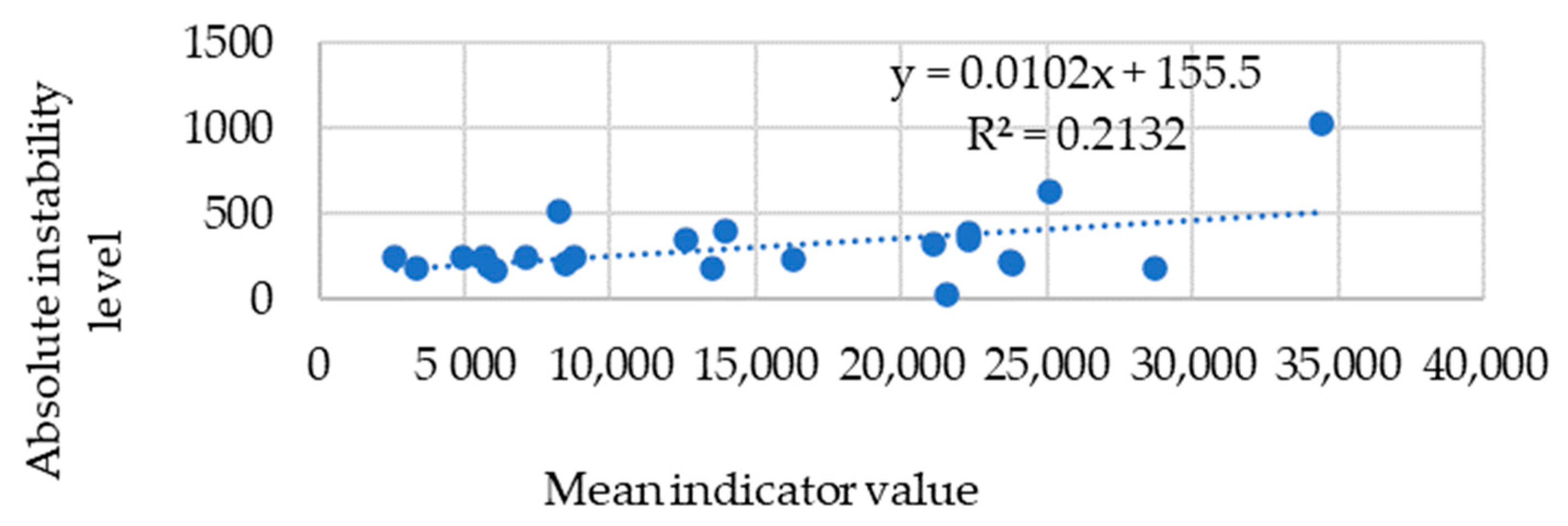
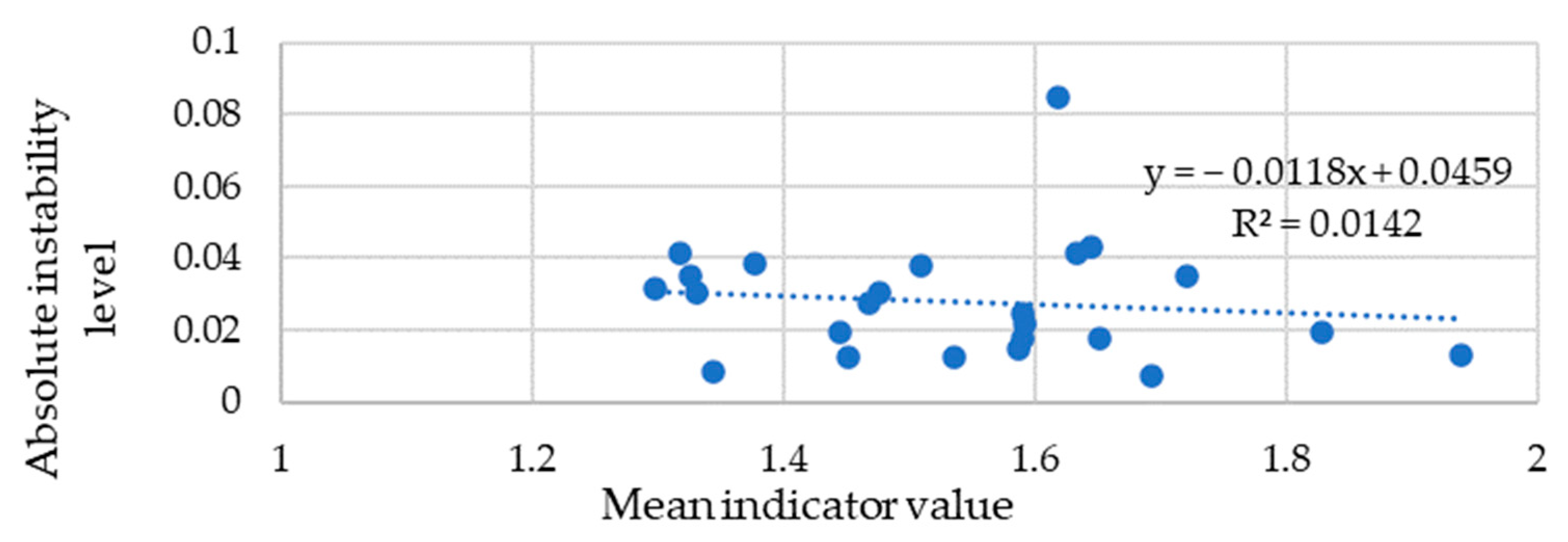
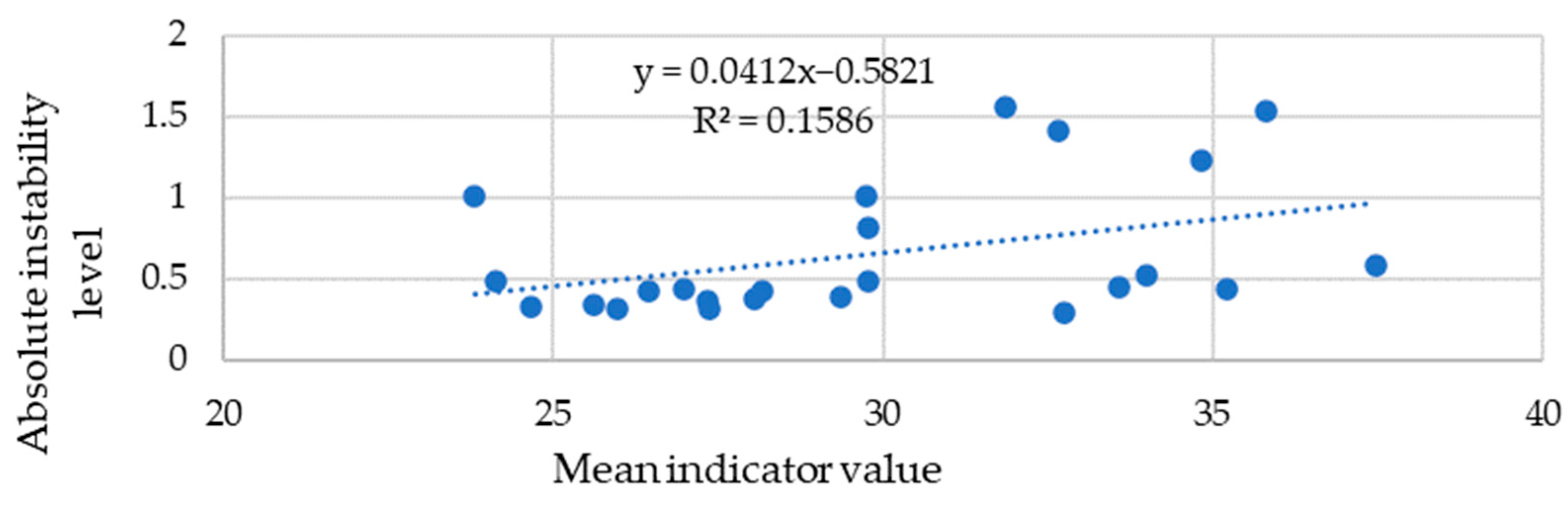
4.1.1. Absolute Instability of the EU Countries Social Development: Individual Indicators Analysis
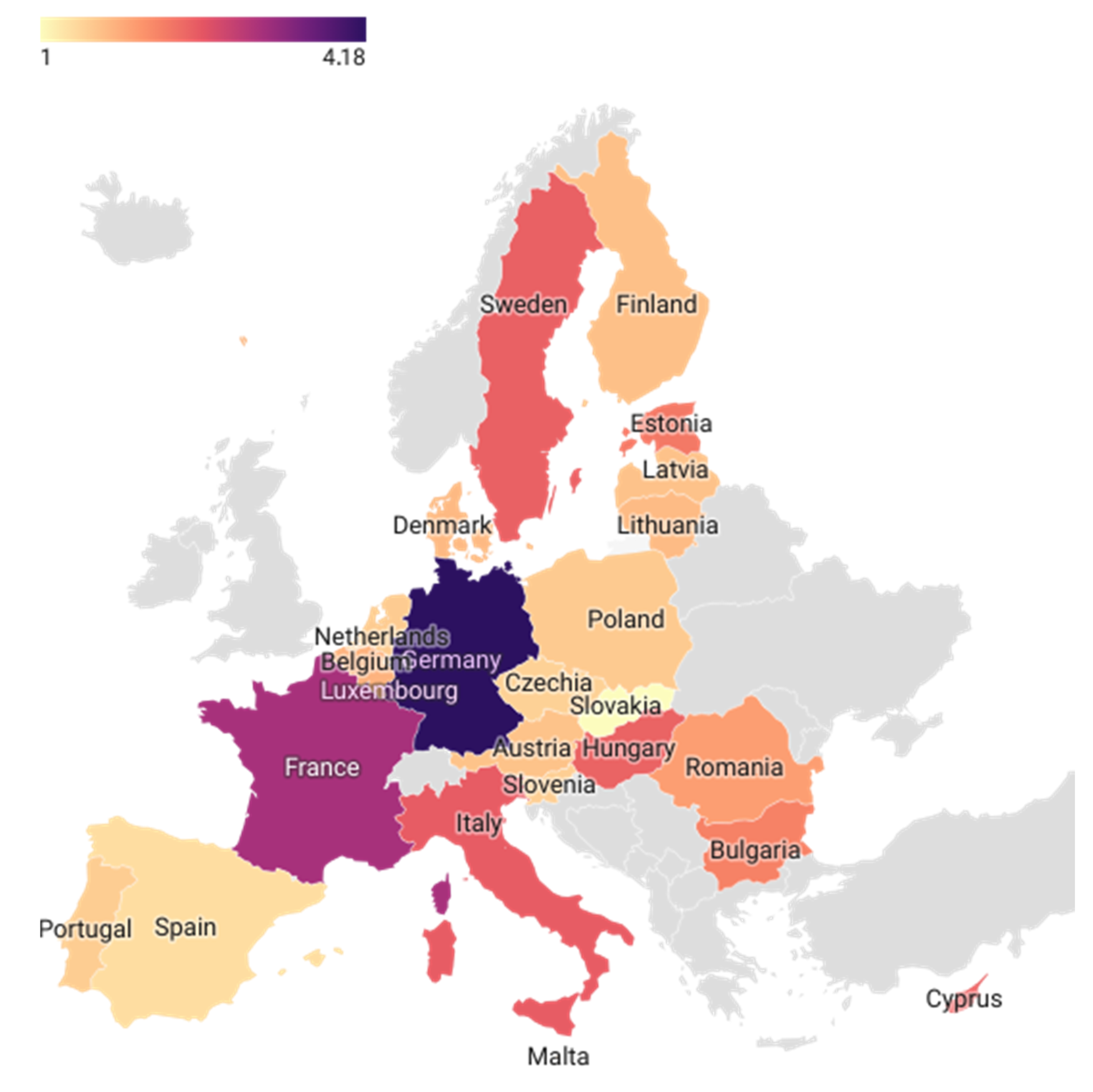
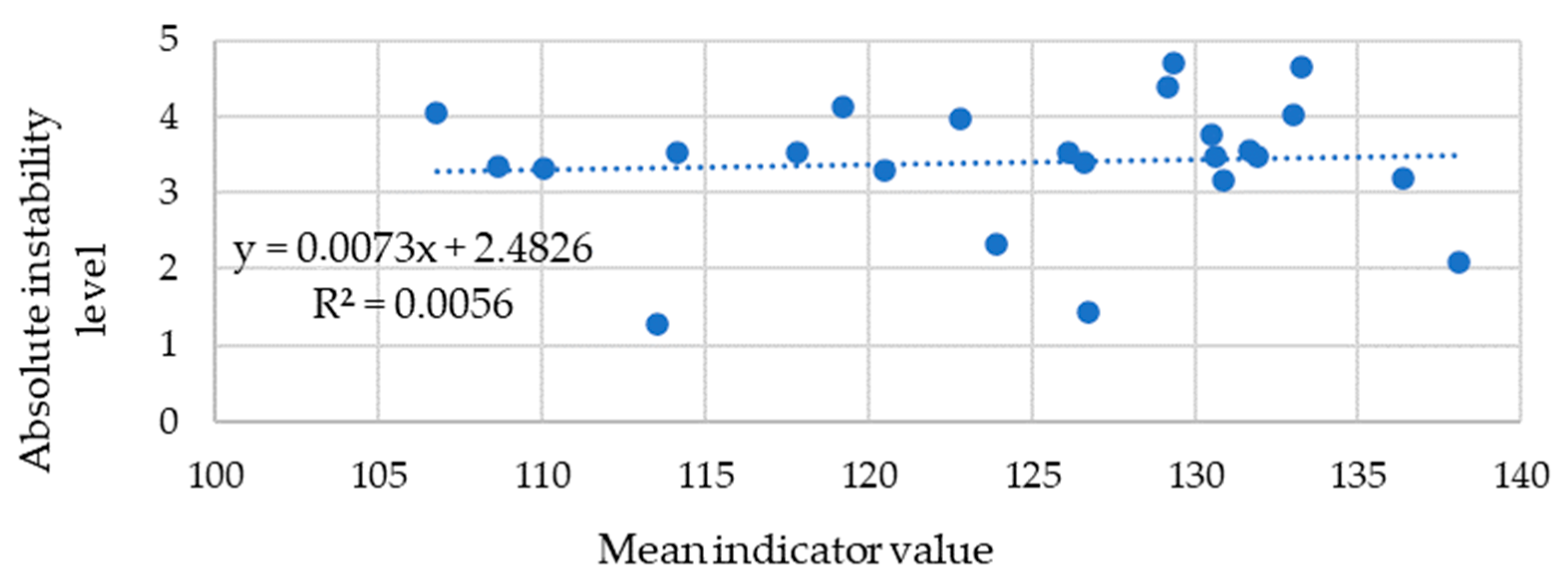
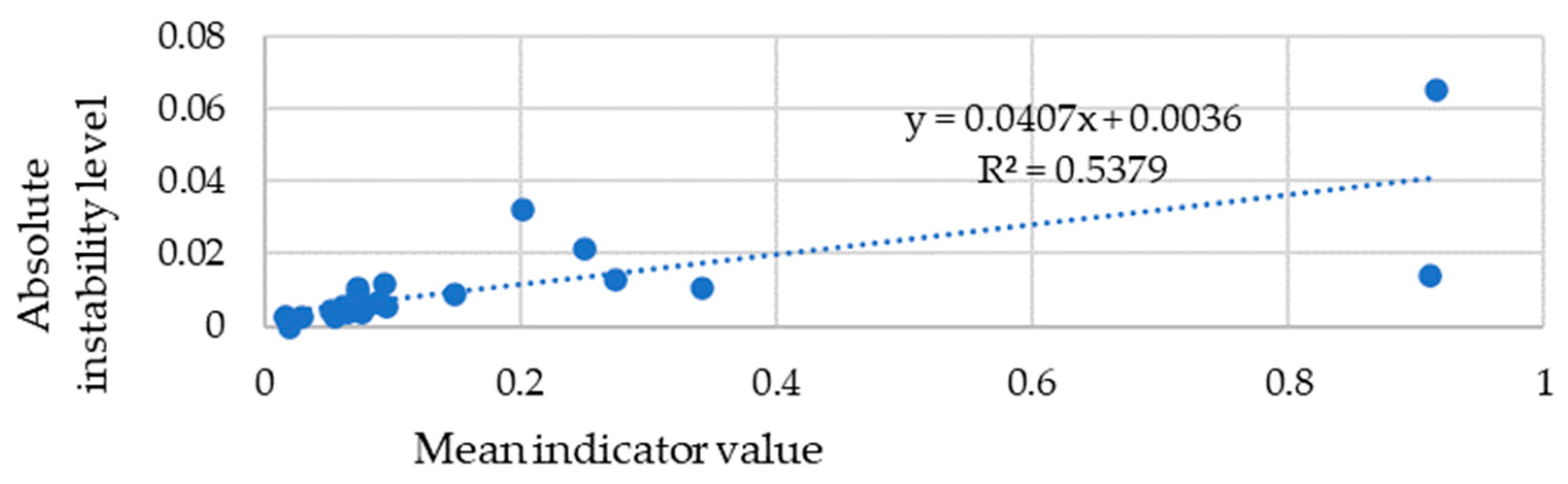
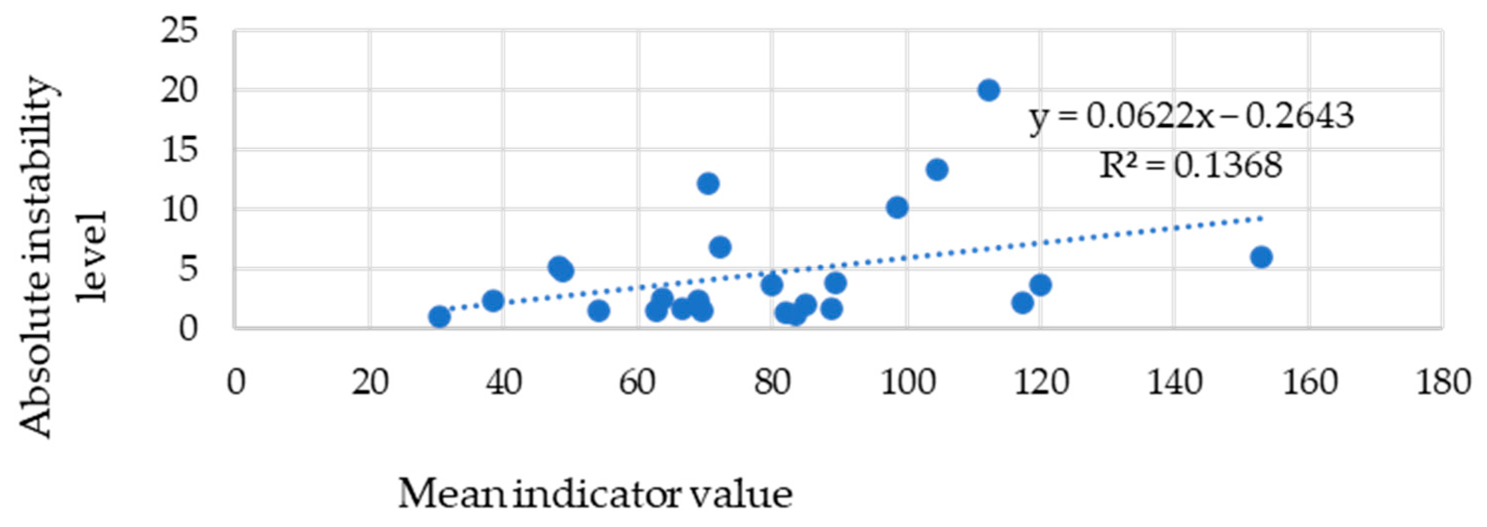
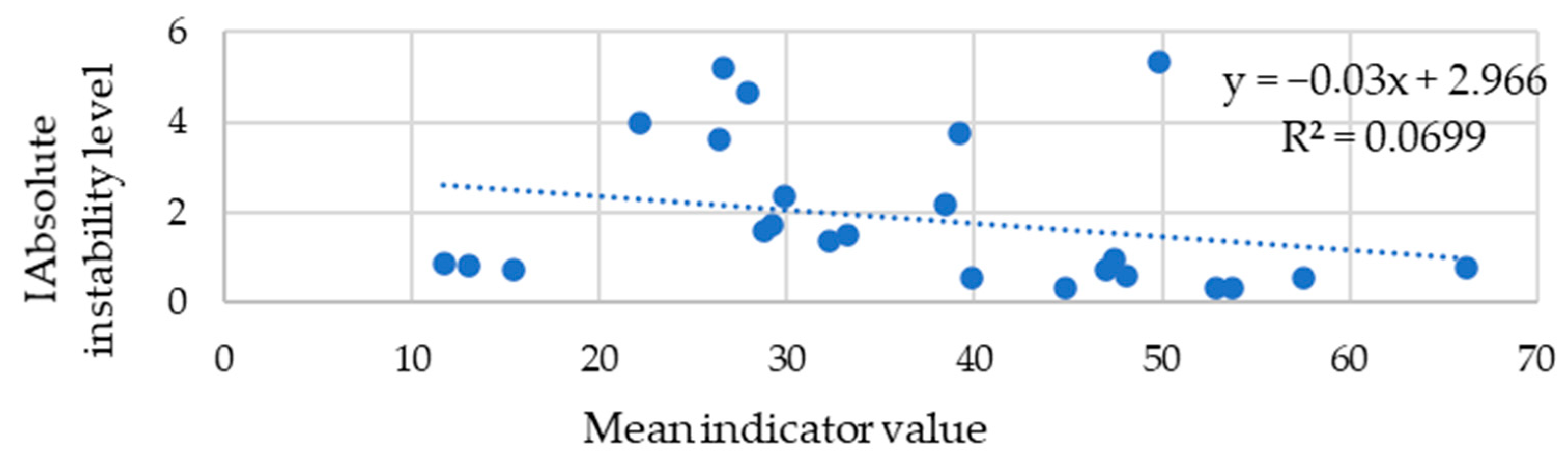
4.1.2. Absolute Instability of the EU Countries Environmental Development: Individual Indicators Analysis
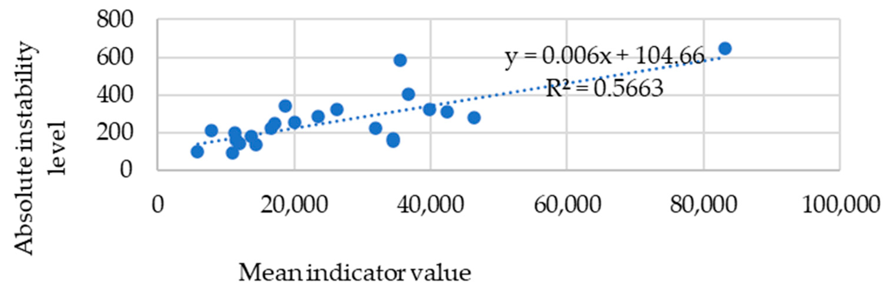
4.1.3. Absolute Instability of the EU Countries Economic Development: Individual Indicators Analysis
4.1.4. The Results of the Analysis of the EU Countries Composite Sustainability Indexes Are Summarized in Table 6

| Indicator | Description | R2 Coefficients of Determination |
|---|---|---|
| Social development | ||
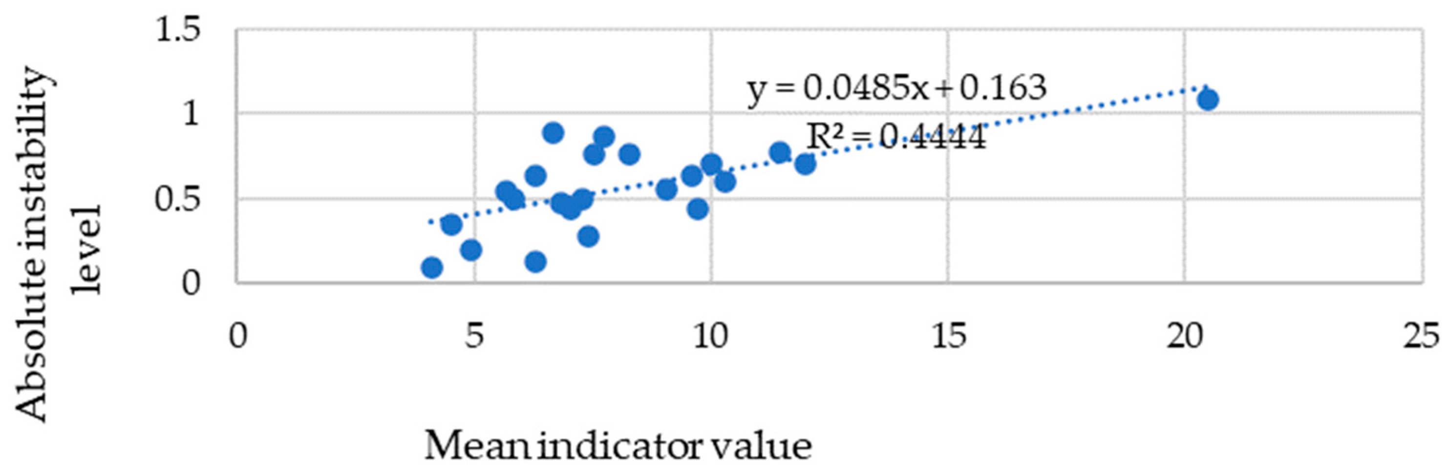
| Unemployment rate, % | The absolute minimum instability was recorded in Germany and the maximum in Cyprus. | R2 = 0.4444 |
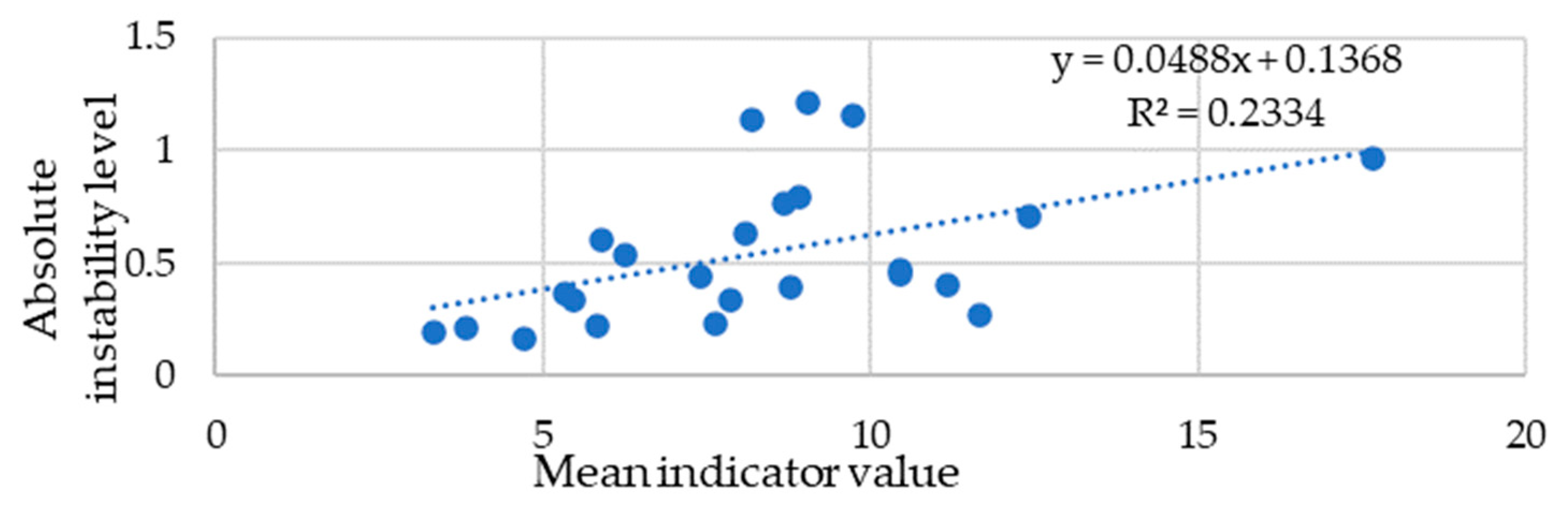
| Working poverty rate, % | The maximum level of instability is reached in Bulgaria, while the most stable countries are Belgium. | R2 = 0.2334 |
| Average and median income by age and sex, euros | France is the most stable country in terms of average and median income, while Cyprus is the most instable. | R2 = 0.2132 |
| Fertility rates by age group | The highest instability is in Latvia and the lowest in Belgium. | R2 = 0.0142 |
| Gini coefficient of equivalent disposable income, scale from 0 to 100 | The most unstable country is Cyprus and the most stable is Italy. | R2 = 0.1586 |
| Environmental development | ||
| Primary energy consumption, million tons of oil equivalent | The absolute minimum instability was recorded in Germany and the maximum in Malta. | R2 = 0.8237 |
| Average CO2 emissions per kilometer from new passenger cars | The highest instability is in Cyprus and the lowest in Malta. | R2 = 0.0056 |
| Emissions intensity from industry, grams per euro | Germany is the most stable in terms of emission intensity, while Estonia has the highest level of instability. | R2 = 0.5379 |
| Net greenhouse gas emissions | The highest instability is in Slovenia, the lowest in Lithuania. | R2 = 0.1368 |
| Recycling rate of municipal waste, % | Slovenia has the maximum level of instability, and the Netherlands is the most stable. | R2 = 0.0699 |
| Economic development | ||
| Real GDP per capita, euros per capita | Cyprus has the highest instability of this indicator, while Latvia has the lowest one. Relative volatility is high in Cyprus, Romania, and Slovenia. A significant positive correlation between real GDP per capita and its absolute instability was found. | R2 = 0.5663 |
| House price index, annual average | The lowest instability is found in Sweden and Finland, explained by high living standards and social infrastructure, government programs, and relatively low population density. The highest instability is observed in Hungary. | R2 = 0.7523 |
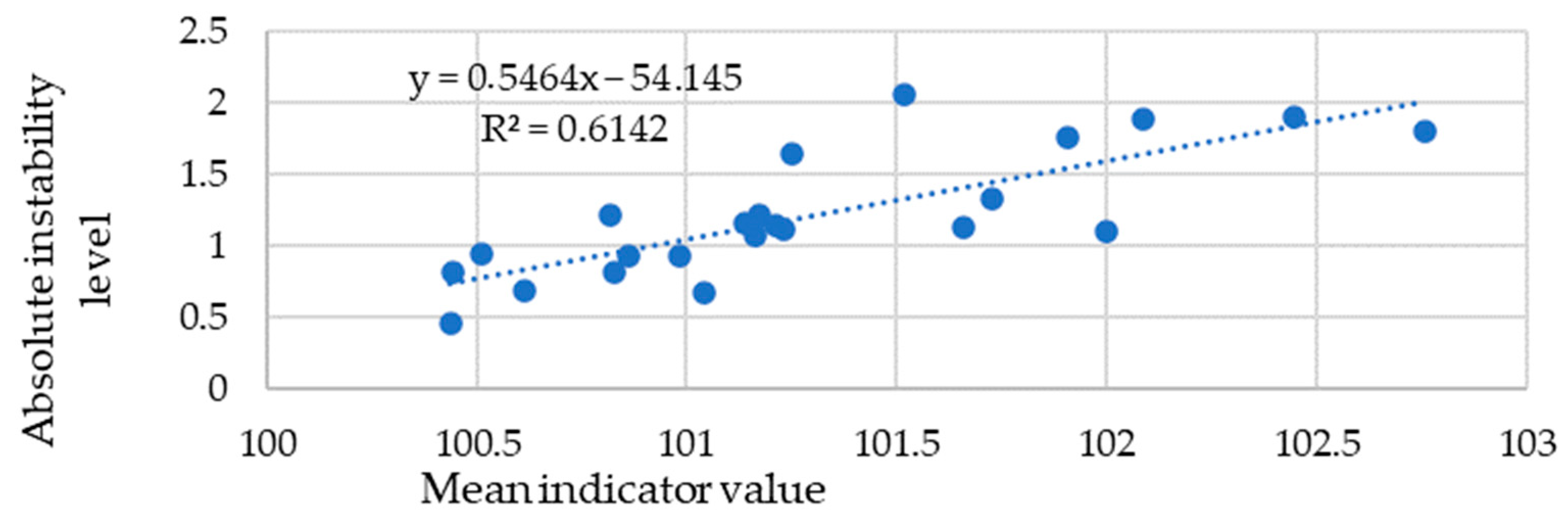
| Harmonized Index of Consumer Prices, average annual index | The most sustainable economy by this criterion is Denmark, the least sustainable is Romania. | R2 = 0.6142 |
| Compensation of employees, million euros | France has the lowest level of instability; Malta has the biggest one. | R2 = 0.7336 |
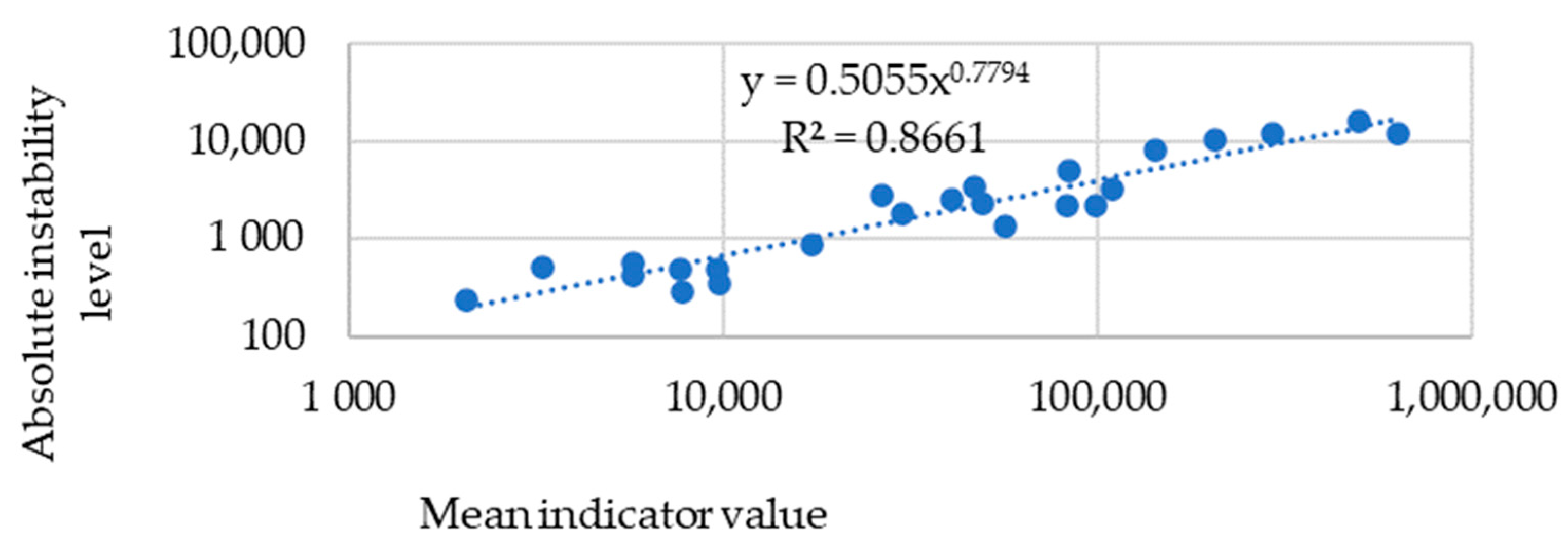
| Gross fixed capital formation, million euros | Lithuania has the lowest level of instability; Slovenia has the biggest one. | R2 = 0.8661 |
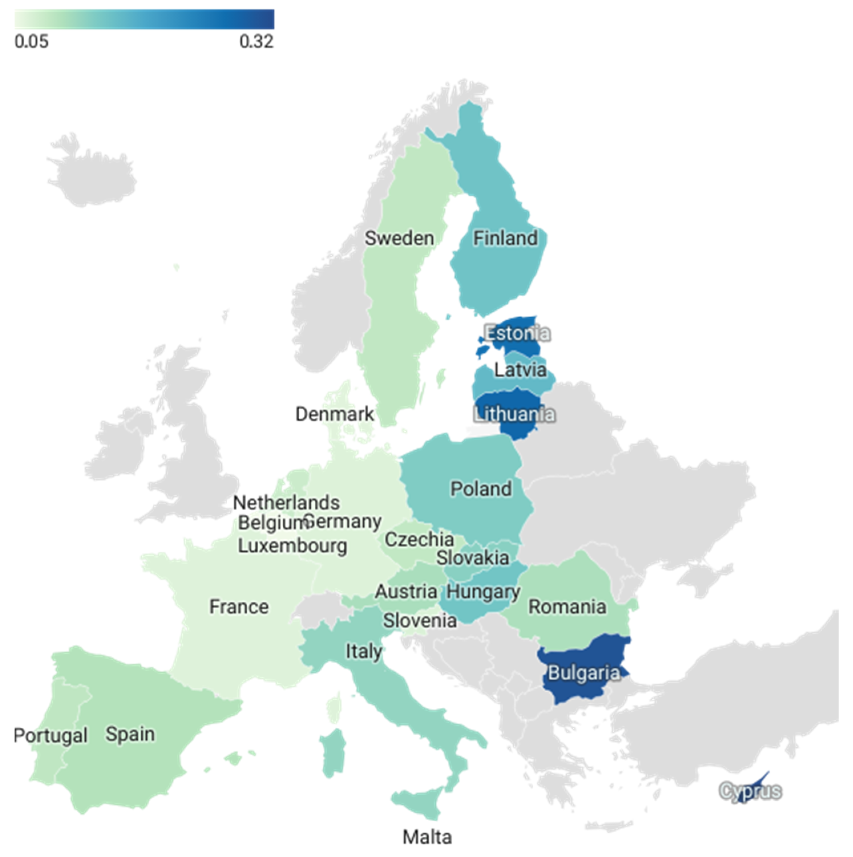
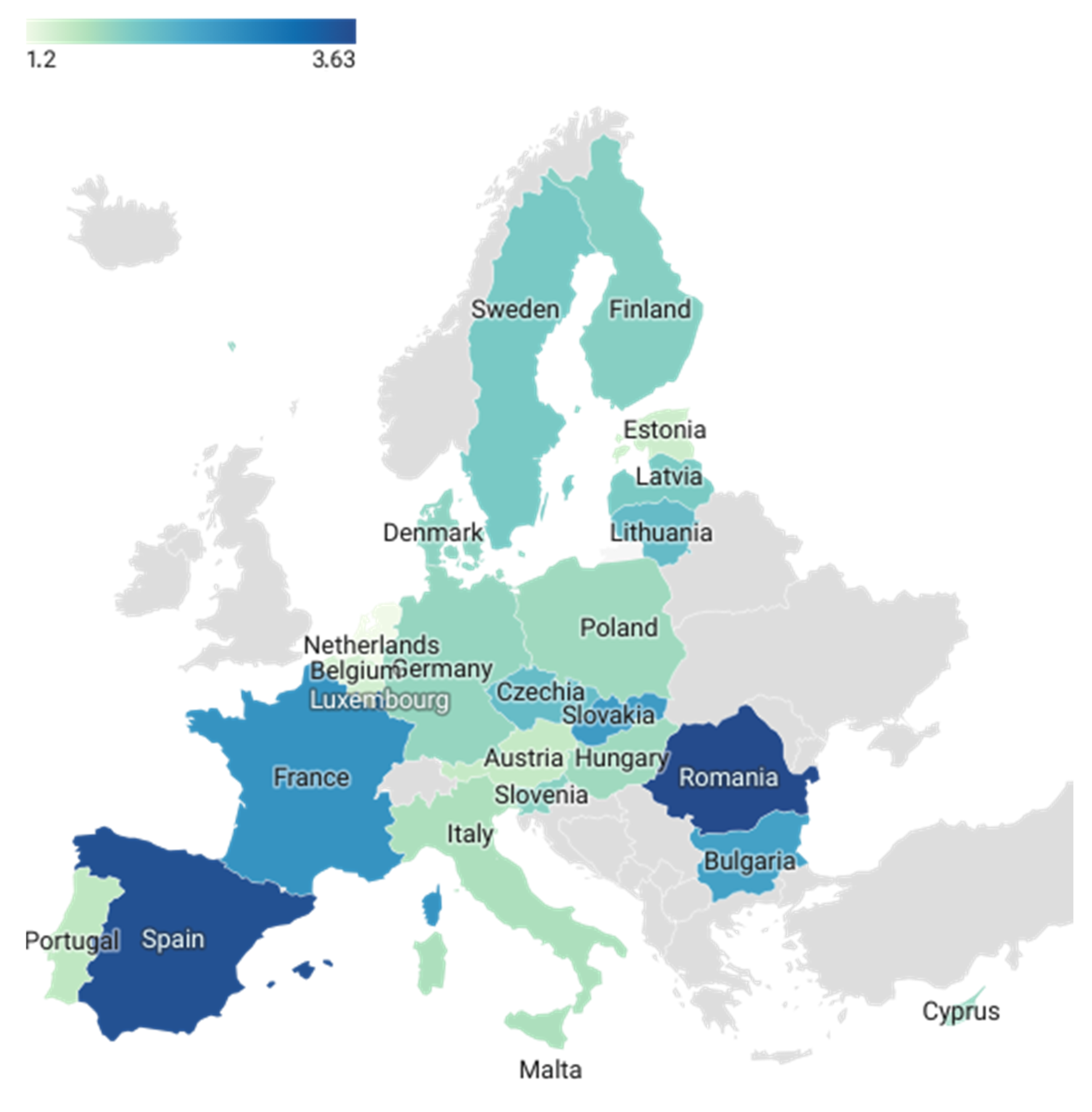
4.2. Countries Clustering by Instability Level and Mahalonobis Distance
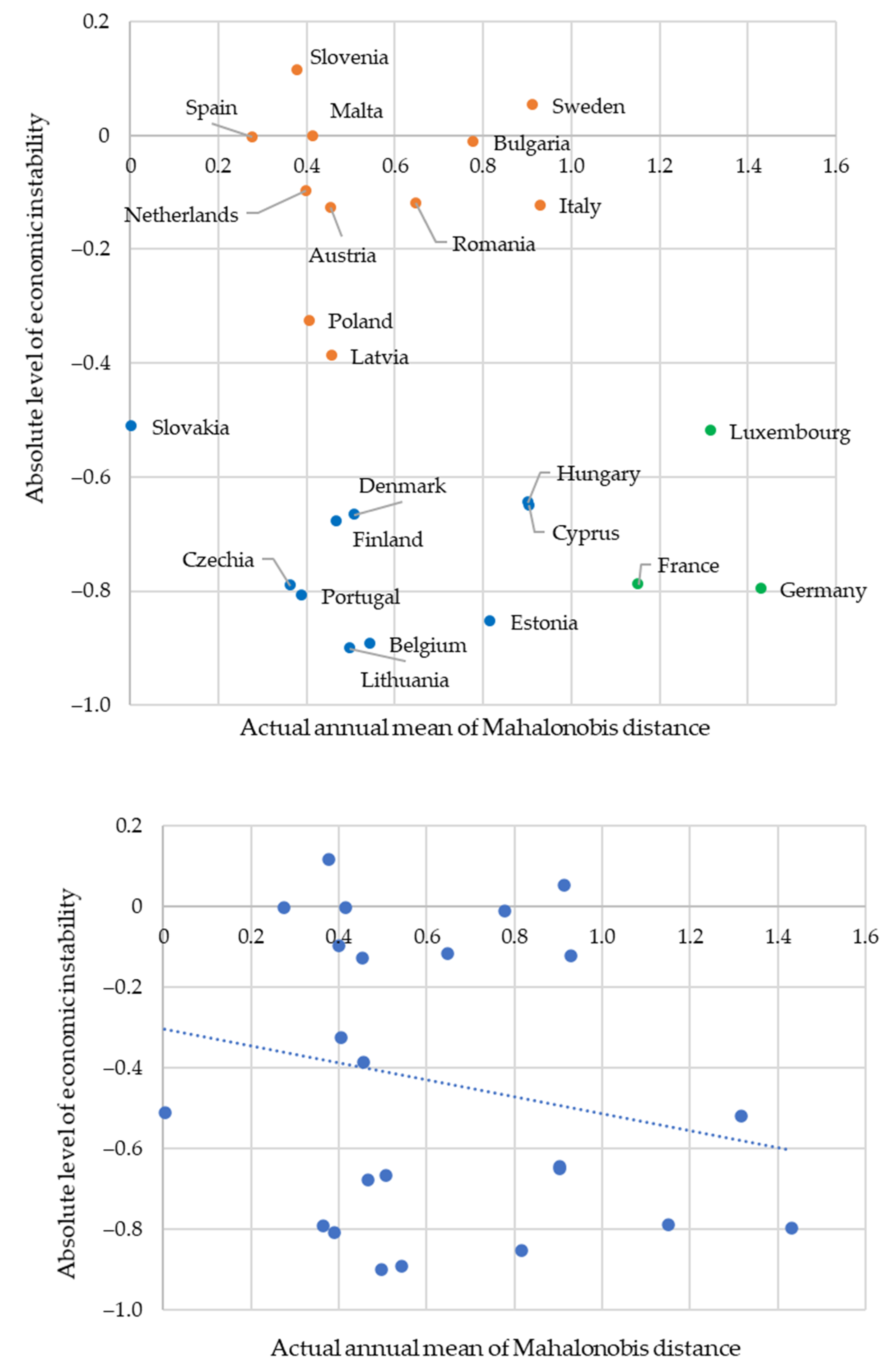
4.2.1. Economic Instability and Mahalonobis Distance
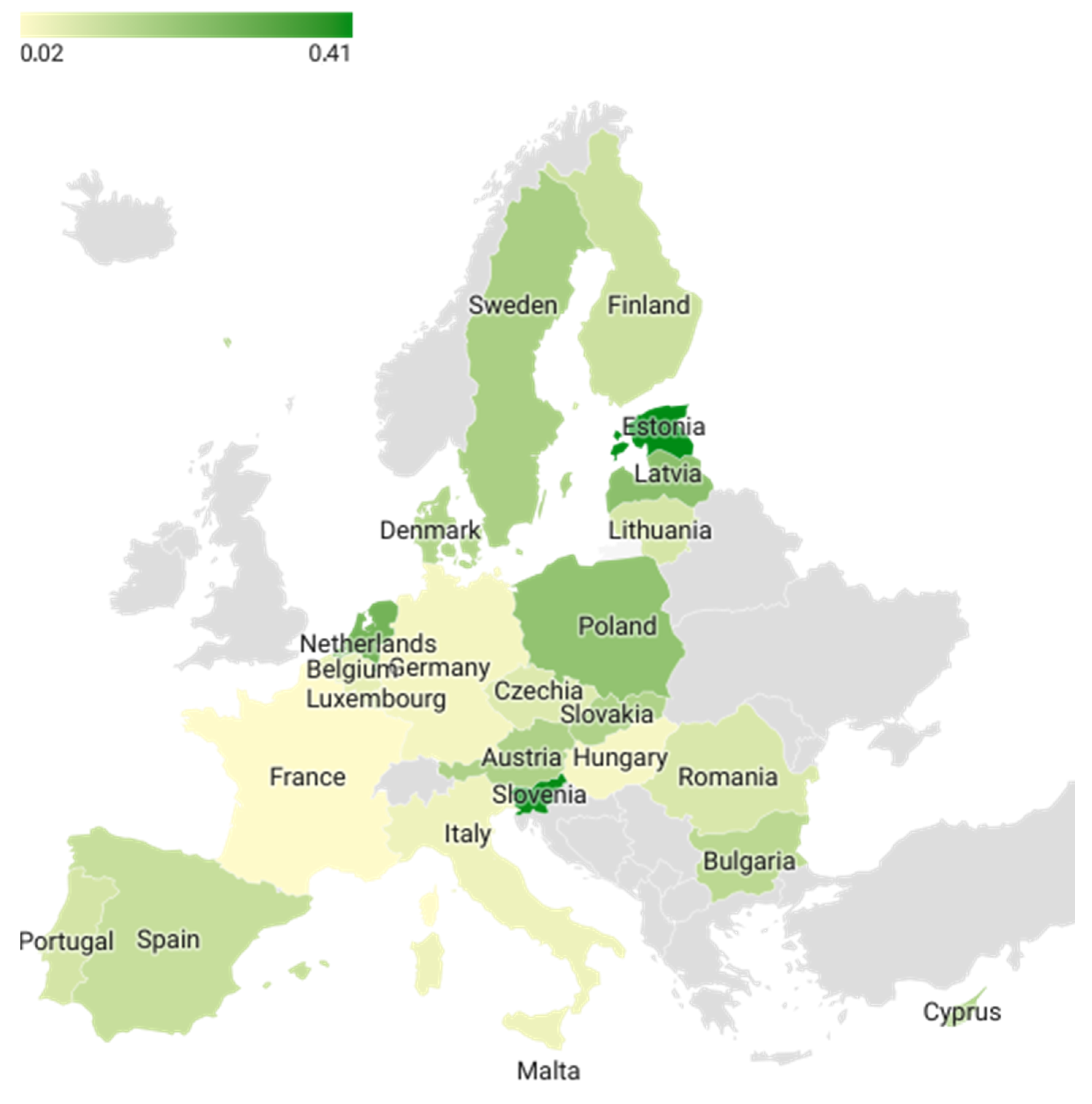
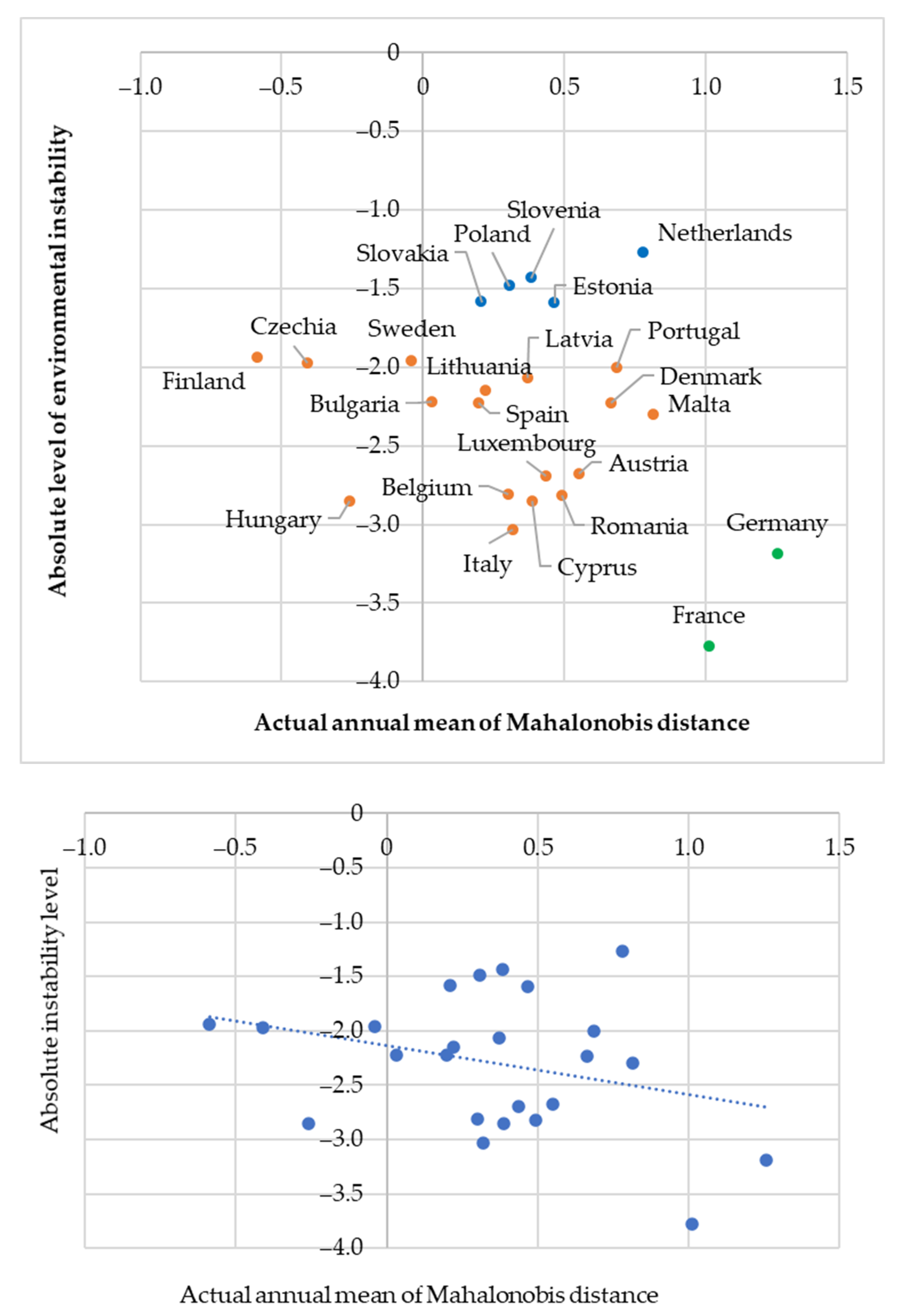
4.2.2. Environmental Instability Mahalonobis Distance
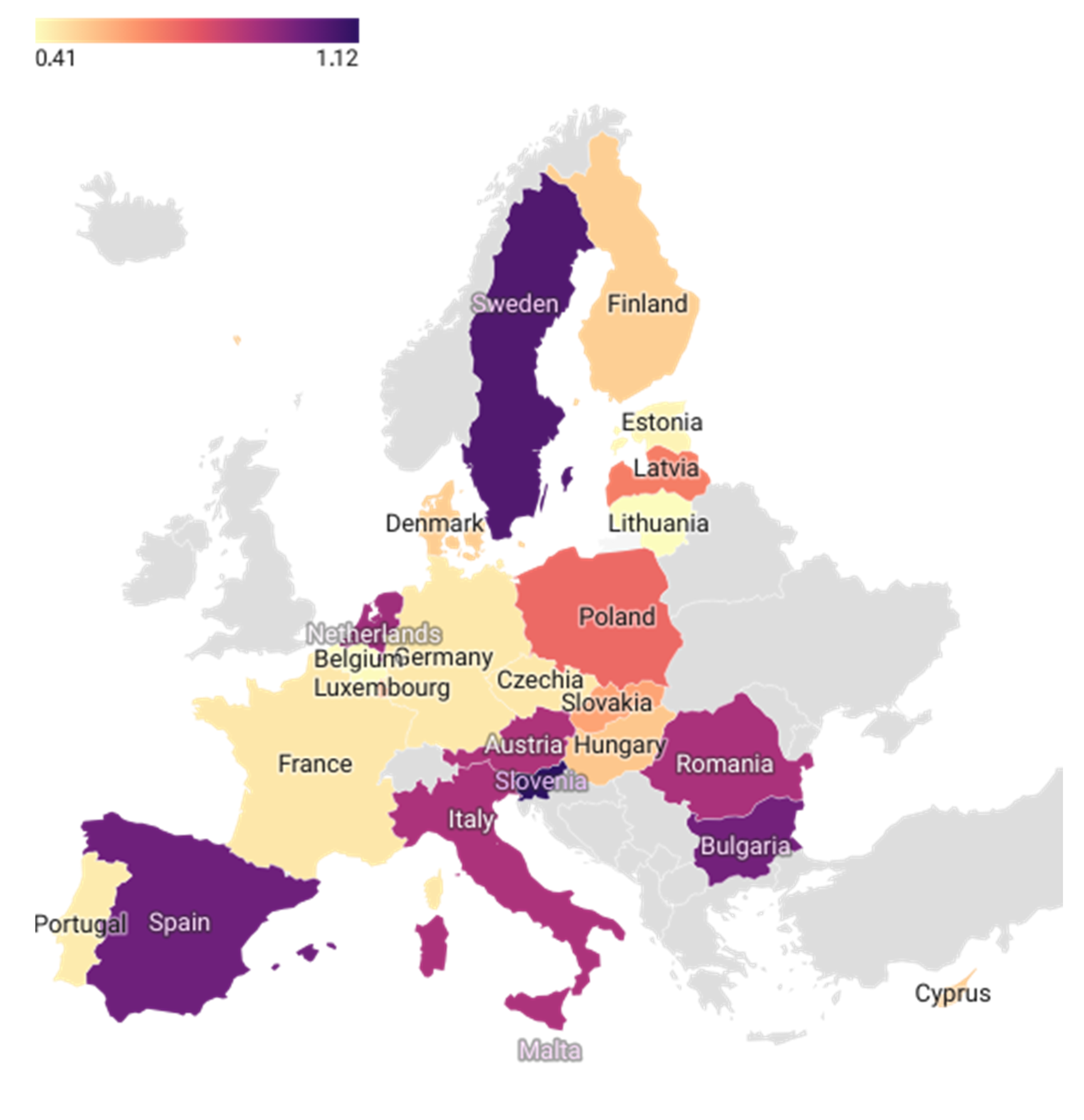
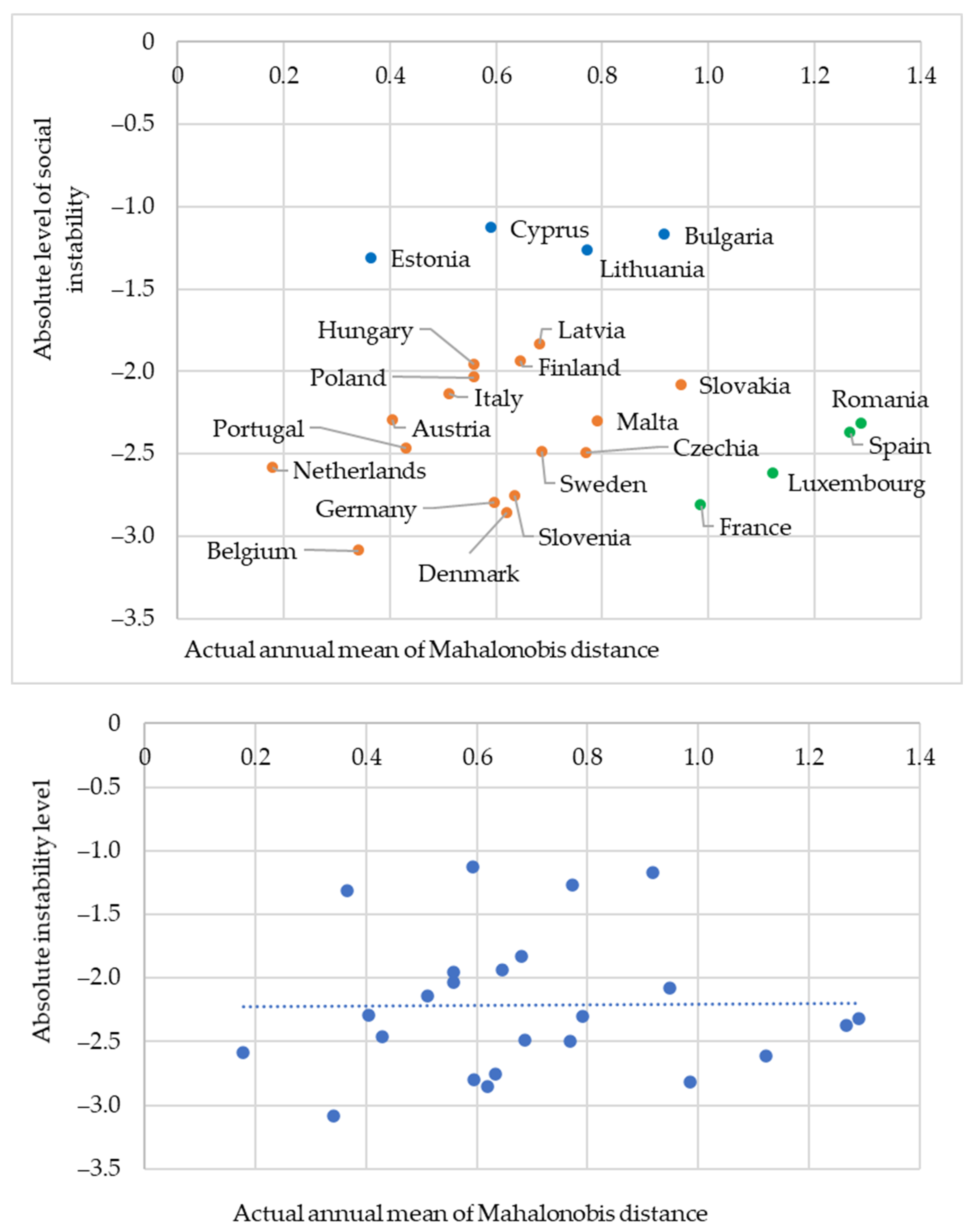
4.2.3. Social Instability and Mahalonobis Distance
5. Conclusions
- Currently, there is no single methodological math approach for sustainability assessment of countries and territorial entities. This is caused predominantly by the different in existing concepts, the applied mathematics indicators and them conceptual content, and variety of unit measurement. In addition, new types of sustainability are appearing now, making sustainable development a complex and multifaceted concept encompassing various dimensions.
- The barrier to practical usage of mathematical models to countries resilience and sustainability assessing is the complexity of the managerial usage of composite indicators, when determining the contribution of individual sustainability factors represents an ambiguity task. The problem of comparative analysis of sustainability is the lack of harmonized statistical data, due to the heterogeneity of countries development.
- To form the policy of sustainable development management, the core of approaches to assessing countries sustainability should be the principles of simultaneous consideration of social, environmental, and economic aspects, as well as possibility to identify meaningful variables in composite indices. In order to make sustainability a target variable in development strategies, it is necessary to use special methods combining mathematical tools and reasonable managerial content.
- A methodological approach consisting of seven successive stages to integrated assessment of social, economic, and environmental sustainability of countries has been created. It allows us to define position of European countries in sustainable development content relative to each other. An approach considers the requirements dictated by the multidimensionality of the studied economic, social, and environmental space and allows us to present the results of the comparative analysis visually, as well as to determine the direction of sustainability management for each country. The instrumental basis of methodological approach consists of multivariate comparisons, the Mahalanobis distances method, the correlation and regression analysis, analysis of variance, time series analysis and trends analysis.
- Composite indices of social, economic, and environmental sustainability of the EU countries, each of them including five indicators, were developed in this study. Developed indices considering multidimensionality features of used data allows us to identify countries dynamics in achieving sustainable development goals. For assessing economic sustainability, Real GDP per capita, House price index, Harmonized Index of Consumer Prices, Compensation of employees, and Gross fixed capital formation were chosen to create a composite index. For assessing environmental sustainability, primary energy consumption, average CO2 emissions per kilometer from new passenger cars, emissions intensity from industry, net greenhouse gas emissions, and recycling rate of municipal waste were chosen to create a composite index. For assessing social sustainability, unemployment rate, working poverty rate, average and median income by age and sex, fertility rates by age group, and Gini coefficient of equivalent disposable income were chosen to create a composite index.
- The sustainability of each indicator in each group (environmental, social, and economic) has been divided into two components: growth rate and fluctuations. The growth rate is a constant component and reflects a stable trend of the indicator change. Fluctuation, on the other hand, is a nonconstant component and reflects the variability of the indicator around the trend. This variability can be measured by volatility, i.e., fluctuations of the indicator around its average value. Thus, analyzing the stability of indicators allows us to divide the dynamics into a stable trend and the risk associated with fluctuations of the indicator around this trend.
- To create a common composite index for each group (environmental, social, and economic), Mahalanobis distances were calculated based on chosen indicators. The methodology is the finding of the average distance between the multivariate vector containing the values of all private indicators and the center of the multivariate distribution. This made it possible to assess how much each private indicator contributes to the overall sustainability score and to determine which indicators are most important.
- A linear time regression analysis has been conducted to identify four main parameters (deviation of the country from the countries mean, sustainable rate of development of the country, absolute level of the countries’ instability, and relative level of instability). This analysis assessed the relationship between various indicators such as the deviation of the country from the countries mean, the sustainable rate of development of the country, the absolute level, and the relative level of country’s instability.
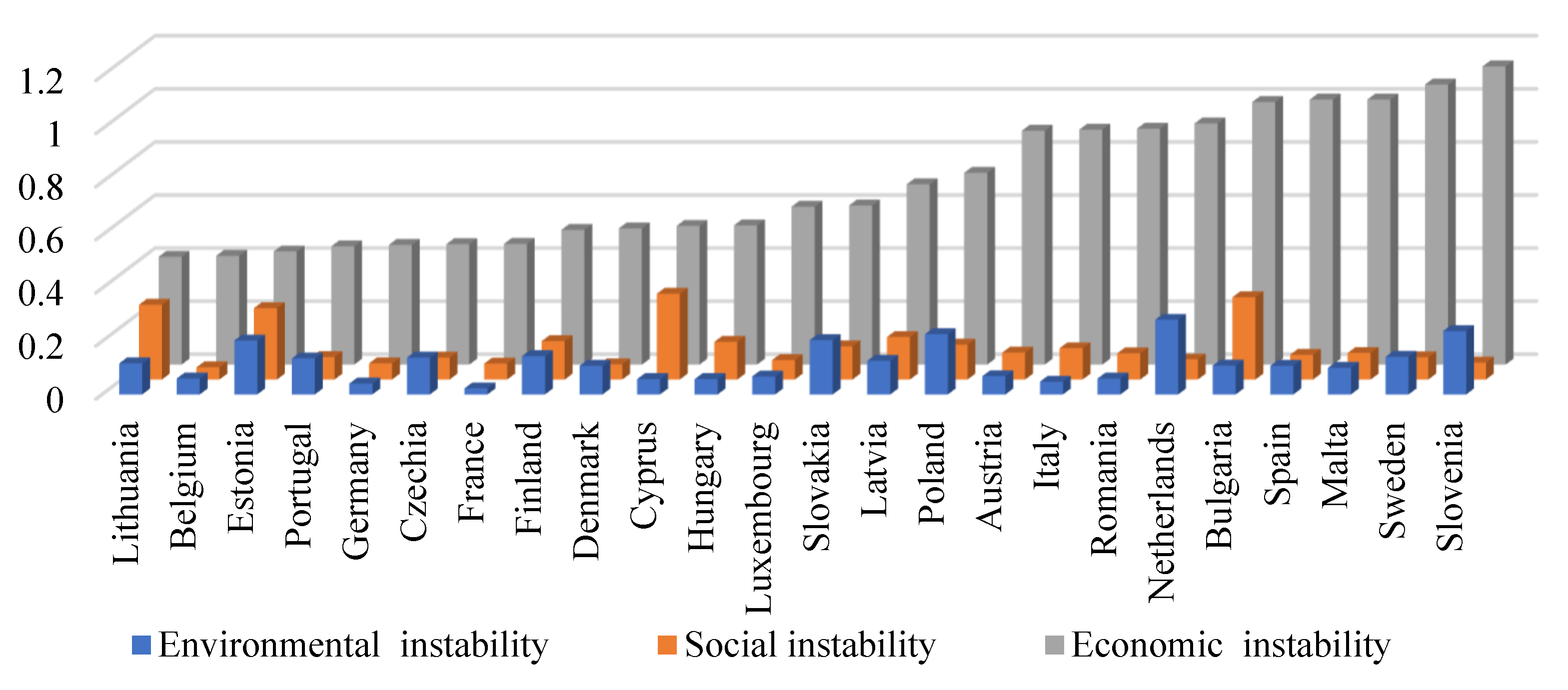
- Based on the Eurostat’s 12-year period data, the levels of social, economic, and environmental sustainability of 24 EU countries were determined. Individual instability indicators of 15 chosen indicators were determined and analyzed. Mahalanobis distances, relative, and absolute instability levels of each composite indexes were calculated (social, economic, and environmental). The most and least sustainable countries for each component of sustainable development were identified. The case study results derived from spatial and temporal samples are consistent with the currently observed processes in the EU. Developed visual representation of the case study results were made.
- Hypotheses that there are positive relationships between instability and the level of country development, reflected in the values of socio-economic and environmental indicators, were proposed and tested. According to the analysis result of positive relationships were revealed for all five economic development indicators, for two environmental indicators. There were no significant positive relationships found for social indicators. As a result of the analysis, the role of economic factors as having more significant impact on the stability of a situation were confirmed.
- The study used several methods, including Mahalanobis distances analysis, time series, trends analysis, correlation and regression analysis, cluster analysis, and analysis of variance. The conducted cluster analysis made it possible to identify three groups of countries depending on Mahalanobis distance and the level of socio-ecological and economic instability. It has been revealed that there are countries with a high Machalanobis distance and a low level of environmental, social, and economic instability.
Author Contributions
Funding
Data Availability Statement
Conflicts of Interest
References
- Foster, K.A. A Case Study Approach to Understanding Regional Resilience; Working Paper 2007-08; Institute of Urban and Regional Development, University of California: Berkeley, CA, USA, 2007. [Google Scholar]
- Olawumi, T.O.; Chan, D.W.M. Identifying and prioritizing the benefits of integrating BIM and sustainability practices in construction projects: A Delphi survey of international experts. Sustain. Cities Soc. 2018, 40, 16–27. [Google Scholar] [CrossRef]
- Da Pimentel Silva, G.D.; Sherren, K.; Parkins, J.R. Using news coverage and community-based impact assessments to understand and track social effects using the perspectives of affected people and decision makers. J. Environ. Manag. 2021, 298, 113467. [Google Scholar] [CrossRef]
- Modica, M.; Reggiani, A. Spatial Economic Resilience: Overview and Perspectives. Netw. Spat. Econ. 2014, 15, 211–233. [Google Scholar] [CrossRef]
- Martin, R. Regional economic resilience, hysteresis and recessionary shocks. J. Econ. Geogr. 2012, 12, 1–32. [Google Scholar] [CrossRef]
- Van Bergeijk, P.A.G.; Brakman, S.; Van Marrewijk, C. Heterogeneous economic resilience and the great recession’s world trade collapse. Pap. Reg. Sci. 2017, 96, 3–12. [Google Scholar] [CrossRef]
- Giannakis, E.; Bruggeman, A. Regional disparities in economic resilience in the European Union across the urban-rural divide. Reg. Stud. 2019, 54, 1200–1213. [Google Scholar] [CrossRef]
- Volkov, A.; Žičkienė, A.; Morkunas, M.; Baležentis, T.; Ribašauskiene, E.; Streimikiene, D.A. Multi-Criteria Approach for Assessing the Economic Resilience of Agriculture: The Case of Lithuania. Sustainability 2021, 13, 2370. [Google Scholar] [CrossRef]
- Donkor, F.K.; Mitoulis, S.-A.; Argyroudis, S.; Aboelkhair, H.; Canovas, J.A.B.; Bashir, A.; Cuaton, G.P.; Diatta, S.; Habibi, M.; Hölbling, D.; et al. SDG Final Decade of Action: Resilient Pathways to Build Back Better from High-Impact Low-Probability (HILP) Events. Sustainability 2022, 14, 15401. [Google Scholar] [CrossRef]
- Lyaskovskaya, E.A. Digitalization of the Russian Federation: A Study of Regional Aspects of Digital Inclusion. Bull. S. Ural. State Univ. Ser. Econ. Manag. 2021, 15, 45–56, In Russian. [Google Scholar] [CrossRef]
- Lyaskovskaya, E.A. Economic sustainability of an enterprise in the context of digital economy. Bull. S. Ural. State Univ. Ser. Econ. Manag. 2022, 16, 87–99, In Russian. [Google Scholar] [CrossRef]
- Lyaskovskaya, E.A. Digitalization, labor market and economic development. Bull. South Ural. State Univ. Ser. Econ. Manag. 2022, 16, 192–196, In Russian. [Google Scholar] [CrossRef]
- United Nations Statistical Division. Discussion Paper on Principles of Using Quantification to Operationalize the SDGs and Criteria for Indicator Selection; EGM on the Indicator Framework: New York, NY, USA, 2015. [Google Scholar]
- Hák, T.; Janoušková, S.; Moldan, B. Sustainable Development Goals: A Need for Relevant Indicators. Ecol. Indic. 2016, 60, 565–573. [Google Scholar] [CrossRef]
- Nishitani, K.; Nguyen, T.B.H.; Trinh, T.Q.; Wu, Q.; Kokubu, K. Are corporate environmental activities to meet sustainable development goals (SDGs) simply greenwashing? An empirical study of environmental management control systems in Vietnamese companies from the stakeholder management perspective. J. Environ. Manag. 2021, 296, 113364. [Google Scholar] [CrossRef]
- Panchal, R.; Singh, A.; Diwan, H. Does circular economy performance lead to sustainable development?—A systematic literature review. J. Environ. Manag. 2021, 293, 112811. [Google Scholar] [CrossRef]
- Dijkstra-Silva, S.; Schaltegger, S.; Beske-Janssen, P. Understanding positive contributions to sustainability. A systematic review. J. Environ. Manag. 2022, 320, 115802. [Google Scholar] [CrossRef]
- Wang, D.; Chen, S. Digital Transformation and Enterprise Resilience: Evidence from China. Sustainability 2022, 14, 14218. [Google Scholar] [CrossRef]
- Kakderi, C.; Tasopoulou, A. Regional economic resilience: The role of national and regional policies. Eur. Plan. Stud. 2017, 25, 1435–1453. [Google Scholar] [CrossRef]
- Duran, H.E.; Fratesi, U. Employment volatility in lagging and advanced regions: The Italian case. Growth Change J. Urban Reg. Policy. 2020, 51, 207–233. [Google Scholar] [CrossRef]
- Rahma, H.; Fauzi, A.; Juanda, B.; Widjojanto, B. Development of a Composite Measure of Regional Sustainable Development in Indonesia. Sustainability 2019, 11, 5861. [Google Scholar] [CrossRef]
- Mai, X.; Chan, R.C.K.; Zhan, C. Which Sectors Really Matter for a Resilient Chinese Economy? A Structural Decomposition Analysis. Sustainability 2019, 11, 6333. [Google Scholar] [CrossRef]
- Rios, V.; Gianmoena, L. The link between quality of government and regional resilience in Europe. J. Policy Model. 2020, 42, 1064–1084. [Google Scholar] [CrossRef]
- Sondermann, D. Towards more resilient economies: The role of well-functioning economic structures. J. Policy Model. 2018, 40, 97–117. [Google Scholar] [CrossRef]
- Kitsos, A.; Carrascal-Incera, A.; Ortega-Argilés, R. The Role of Embeddedness on Regional Economic Resilience: Evidence from the UK. Sustainability 2019, 11, 3800. [Google Scholar] [CrossRef]
- Chacon-Hurtado, D.; Losada-Rojas, L.L.; Yu, D.; Gkritza, K.; Fricker, J.D. A Proposed Framework for the Incorporation of Economic Resilience into Transportation Decision Making. J. Manag. Eng. 2020, 36, 04020084. [Google Scholar] [CrossRef]
- Pretorius, O.; Drewes, E.; van Aswegen, M.; Malan, G. A Policy Approach towards Achieving Regional Economic Resilience in Developing Countries: Evidence from the SADC. Sustainability 2021, 13, 2674. [Google Scholar] [CrossRef]
- Di Caro, P. Testing and explaining economic resilience with an application to Italian regions. Pap. Reg. Sci. 2015, 96, 93–113. [Google Scholar] [CrossRef]
- Giannakis, E.; Bruggeman, A. Determinants of regional resilience to economic crisis: A European perspective. Eur. Plan. Stud. 2017, 25, 1394–1415. [Google Scholar] [CrossRef]
- Brown, L.; Greenbaum, R.T. The role of industrial diversity in economic resilience: An empirical examination across 35 years. Urban Stud. 2016, 54, 1347–1366. [Google Scholar] [CrossRef]
- Zeng, X.; Yu, Y.; Yang, S.; Lv, Y.; Sarker, M.N.I. Urban Resilience for Urban Sustainability: Concepts, Dimensions, and Perspectives. Sustainability 2022, 14, 2481. [Google Scholar] [CrossRef]
- Yu, H.; Liu, Y.; Liu, C.; Fan, F. Spatiotemporal Variation and Inequality in China’s Economic Resilience across Cities and Urban Agglomerations. Sustainability 2018, 10, 4754. [Google Scholar] [CrossRef]
- Ahmad, T.; Thaheem, M.J. Developing a residential building-related social sustainability assessment framework and its implications for BIM. Sustain. Cities Soc. 2017, 28, 1–15. [Google Scholar] [CrossRef]
- Ahmadian, F.F.A.; Rashidi, T.H.; Akbarnezhad, A.; Waller, S.T. BIM-enabled sustainability assessment of material supply decisions. Eng. Constr. Arch. Manag. 2017, 24, 668–695. [Google Scholar] [CrossRef]
- Ramos, T.; Pires, S.M. Sustainability Assessment: The Role of Indicators. In Sustainability Assessment Tools in Higher Education Institutions: Mapping Trends and Good Practices Around the World; Caeiro, S., Filho, W., Jabbour, C., Azeiteiro, U., Eds.; Springer International Publishing: Cham, Switzerland, 2013; pp. 81–99. ISBN 978-331902375-5. [Google Scholar]
- Büyükozkan, G.; Karabulut, Y. Sustainability performance evaluation: Literature review and future directions. J. Environ. Manag. 2018, 217, 253–267. [Google Scholar] [CrossRef] [PubMed]
- Briguglio, L.; Cordina, G.; Farrugia, N.; Vella, S. Economic vulnerability and resilience: Concepts and measurements. Oxf. Dev. Stud. 2009, 37, 229–247. [Google Scholar] [CrossRef]
- Malkina, M.Y. Sustainability of regional economies and its factors. Nauchnye Tr. Volnogo Ekon. Obs. Ross. 2021, 230, 397–403. [Google Scholar]
- Eurostat. 2022. Available online: https://ec.europa.eu/eurostat/web/main/data/database (accessed on 30 December 2022).
- Ferova, I.S.; Lobkova, E.V.; Tanenkova, E.N.; Kozlova, S.A. Tools for Assessing Sustainable Development of Territories Taking into Account Cluster Effects. J. Sib. Fed. Univ. 2019, 12, 600–626. [Google Scholar] [CrossRef]
- Podol’naya, N.N.; Ryabova, S.G. Sustainability of regional socio-economic systems: Evaluation toolkit and the nature of development. Natl. Interests Priorities Secur. 2017, 13, 827–842. [Google Scholar] [CrossRef]
- Yakovina, M.Y.; Korableva, A.A. Recessionary shocks and regional economic sustainability. Bull. Sib. Inst. Bus. Inf. Technol. 2020, 3, 117–123. [Google Scholar] [CrossRef]


| Sustainability Measurement | Approach | Authors |
|---|---|---|
| Qualitative analysis of sustainability | Impact of the pandemic situation on progress towards the SDGs | [9] |
| Identification of sustainable development targets with a focus on justifying their relevance | [14] | |
| The need to link social, environmental, and economic indicators to the public vision of sustainable development and the UN SDGs | [3,15] | |
| The need for sustainable transformation of markets and society | [16] | |
| The need to identify positive contributions to sustainable development that facilitate stakeholder decision making | [17] | |
| Linking digital transformation and sustainability | [18] | |
| Understanding the political and governance dimensions of sustainability | [19] | |
| Examining resilience and vulnerability through the lenses of evolutionary dynamics and exposure to shocks | [4] | |
| Using the concept of hysteresis to examine the possible responses of the economic system to crisis shocks | [5] | |
| Impact of global shocks on regional resilience | [6] | |
| A theoretical framework for incorporating sustainability indicators into the decision-making process is proposed | [26] | |
| Developing urban resilience indicators: adaptive capacity, absorptive capacity, and transformative capacity | [31] | |
| Quantitative analysis of sustainability | Developing statistical indices: regional resilience to economic shocks and postcrisis recovery | [7] |
| Using three types of measurements: arithmetic mean, geometric mean, and entropy index | [21] | |
| Vector autoregressive modeling and impulse response function (IRF) | [22] | |
| Bayesian Model Averaging (BMA) | [23] | |
| Simple Additive Weighting (SAW) | [8] | |
| Method of residuals of vector autoregression (VAR) | [24] | |
| Econometric panel data methods | [25] | |
| Chi-Square Test of Homogeneity ) | [27] | |
| Autoregression method with smooth transition (STAR) | [28] | |
| Multi-level logistic regression model | [29] | |
| Fixed-effects model | [30] | |
| the Technique for Order of Preference by Similarity to Ideal Solution (TOPSIS) methods | [32] | |
| Multidimensional approach with support for building information modeling (BIM) | [34] | |
| TOPSIS method with application of the structural differences indicator—V.M. Ryabtsev index | [40] | |
| Methods of comparative, abstract-logical and statistical analysis, calculation, and graphic method “radar (polygon) of competitiveness” | [41] | |
| Resistance index and recovery index | [42] |
| Stage Name | Stage Content |
|---|---|
| 1. Informative | Selection of countries to be analyzed |
| 2. Staged | Development and substantiation of composite indices reflecting social, economic and environmental components of sustainability in accordance with the UN concept of sustainable development and the European Union statistical reporting system |
| 3. Statistic | 3.1 Collection of statistical information on indicators included in the social, economic and environmental composite indices 3.2 Testing for the presence of a unit root in panel data using the Dickey–Fuller test: where Δyt is the first difference of the variable of interest at time tt, α is a constant term, βt represents a time trend, γyt − 1 captures the lagged dependent variable, δ1Δyt – 1 + … + δp − 1Δyt – p + 1 includes lagged differences of the variable up to order p − 1p − 1, ϵt is the error term. 4. Aggregation of composite indices and determination of instability levels for each of them as well as for individual indicators via Mahalanobis distances |
| 4. Methodical | 4.1 Construction of x—multidimensional vectors of indicators for each i-th country ( = 1…24) for each j-th (j = 1…5) indicator included in the economic, social, and environmental composite indices, where |
| 4.2 Construction of a vector of mean values for each indicator included in the economic, social, and environmental composite index—. | |
| 4.3 Calculation the inverse covariance matrix of indices | |
| 4.4 Aggregation of indicators included in composite indices. Determination of the Mahalanobis distance— for each i-th country ( in each t-th year () for composite indices—economic, social, and environmental | |
| 4.5 Calculation of —linear time regressions of Mahalanobis distances for each country over the study period (for each aggregate index) and their estimation by the least squares method. | |
| 4.6 Separating of the trend and cyclical component of linear time regressions of Mahalanobis distances for each country over the study period (for each aggregate index) by the least squares method. where и —regression coefficients, —regression residuals | |
| 4.7 Calculation of the absolute level of instability of social, economic, and environmental development of countries through —calculation of the mean square deviation of the residuals of the Mahalanobis distance regression for each country for the period under study. The higher the level of instability, the greater the fluctuations of economic, social, and environmental development of the country relative to its own stable trend. 4.8 Calculation of the relative level of instability of social, economic, and environmental development of countries where —mean of predicted value of Mahalanobis distance (using time series regression). | |
| 5. Analytic | Visualization and analysis of the obtained results on the levels of economic, environmental, and social instability of the EU countries. |
| 6. Verifying | Assessment of the reliability of the obtained results and testing of the hypothesis about the relationship between the instability of countries and the indicators included in the composite indices. |
| 7. Predictive | Using the results of the analysis for decision making. |
| Index | Indicators and Unit of Measure |
|---|---|
| Economic sustainability | Real GDP per capita, euros per capita |
| House price index, annual average | |
| Harmonized Index of Consumer Prices, average annual index | |
| Compensation of employees, million euros | |
| Gross fixed capital formation, million euros | |
| Environmental sustainability | Primary energy consumption, million tons of oil equivalent |
| Average CO2 emissions per kilometer from new passenger cars | |
| Emissions intensity from industry, grams per euro | |
| Net greenhouse gas emissions | |
| Recycling rate of municipal waste, % | |
| Social sustainability | Unemployment rate, % |
| Working poverty rate, % | |
| Average and median income by age and sex, euros | |
| Fertility rates by age group | |
| Gini coefficient of equivalent disposable income, scale from 0 to 100 |
| Country | Indicators and Unit of Measure | ADF Stat | p-Value |
|---|---|---|---|
| Italy | Real GDP per capita, euros per capita | −1.8 | 0.12 |
| Hungary | House price index, annual average | −3.2 | 0.01 |
| Latvia | Average CO2 emissions per kilometer from new passenger cars | −2.5 | 0.003 |
| Cyprus | Working poverty rate | −2.7 | 0.02 |
| Malta | Net greenhouse gas emissions | −0.5 | 0.78 |
| Finland | Gini coefficient of equivalent disposable income, scale from 0 to 100 | −3.5 | 0.005 |
| Romania | Unemployment rate | −1.2 | 0.25 |
| Mahalanobis Distance and Instability Level for Economic Indicators | ||||||||||
|---|---|---|---|---|---|---|---|---|---|---|
| Indicator | Unit of Measure | ) | ||||||||
| Countries Mean | Max/Country | Min/Country | Countries Mean | Max/Country | Min/Country | Countries Mean | Max/Country | Min/Country | ||
| Real GDP per capita | EUR million per capita | 25,713.2292 | 83,187.5 Luxembourg | 5867.5 Bulgaria | 287.9473 | 938.9834 Cyprus | 91.1463 Latvia | 0.0131 | 0.0418 Cyprus | 0.0045 Belgium |
| Housing Price Index | annual average | 106.1273 | 114.5863 Hungary | 100.1538 Sweden | 4.8424 | 11.741 Hungary | 0.5243 Finland | 0.0432 | 0.0939 Hungary | 0.0051 Finland |
| The Harmonized Index of Consumer Prices | Average annual index | 101.2759 | 102.755 Lithuania | 100.4375 Denmark | 1.2522 | 2.3098 Romania | 0.4567 Denmark | 0.0122 | 0.0227 Romania | 0.0045 Denmark |
| Compensation of employees | EUR million | 238,889.7031 | 1,606,473.625 Germany | 4483.8625 Malta | 3822.4075 | 14,869.9583 Germany | 188.1354 Malta | 0.0301 | 0.0841 Cyprus | 0.007 France |
| Gross fixed capital formation | EUR million | 102,966.6484 | 633,044.125 Germany | 2076.375 Malta | 3742.0951 | 15,979.3963 France | 233.7455 Malta | 0.0575 | 0.1541 Cyprus | 0.0195 Germany |
| Economic development instability level (Vei) | 0.6851 | 1.1236 Slovenia | 0.4064 Lithuania | 0.3982 | 0.8446 Slovenia | 0.1064 Germany | ||||
| Mahalonobis distanceeconomic component | Countries mean | Max/country | Min/country | |||||||
| 2.0149 | 4.1842 Germany | 1.003 Slovakia | ||||||||
| Mahalanobis Distance and Instability Level for Environmental Indicators | ||||||||||
| Indicator | Unit of Measure | Predicted Value of Mahalanobis Distance (Time Series Regression) | Relative Level of Instability (Vei) | |||||||
| Countries Mean | Max/Country | Min/Country | Countries Mean | Max/Country | Min/Country | Countries Mean | Max/Country | Min/Country | ||
| Primary energy consumption | mln tons of oil equivalent | 55.1057 | 296.475 Germany | 0.85 Malta | 1.1283 | 4.361 Germany | 0.08 Malta | 0.0297 | 0.0941 Malta | 0.0104 France |
| Average CO2 emissions per km from new passenger cars | - | 124.6589 | 138.075 Estonia | 106.7875 Netherlands | 3.397 | 4.6989 Cyprus | 1.2655 Malta | 0.0274 | 0.0379 Netherlands | 0.0111 Malta |
| Emissions intensity from industry | grams per euro | 0.1949 | 0.915 Latvia | 0.0163 Denmark | 0.0183 | 0.1923 Estonia | 0 Germany | 0.0912 | 0.2876 Estonia | 0 Germany |
| Net GHG emissions | - | 79.5193 | 153.05 Cyprus | 30.4875 Lithuania | 4.6846 | 20.0661 Slovenia | 0.9886 Lithuania | 0.0582 | 0.1788 Slovenia | 0.0147 Belgium |
| Recycling rate of municipal waste | % | 36.713 | 66.175 Germany | 11.675 Malta | 1.8661 | 5.3435 Slovenia | 0.3097 Netherlands | 0.0628 | 0.1958 Latvia | 0.0059 Netherlands |
| Environmental development instability level (Vei) | 0.1195 | 0.2811 Netherlands | 0.0228 France | 0.0936 | 0.26 Finland | 0.0083 France | ||||
| Mahalonobis distance environmental component | - | Countries mean 1.554 | Max/country 3.5119 Denmark | Min/ country 0.5551 Finland | ||||||
| Mahalanobis Distance and Instability Level for Social Indicators | ||||||||||
| Indicator | Unit of Measure | Predicted Value of Mahalanobis Distance (Time Series Regression) | Relative Level of Instability (Vei) | |||||||
| Countries Mean | Max/Country | Min/Country | Countries Mean | Max/Country | Min/Country | Countries Mean | Max/Country | Min/Country | ||
| Unemployment rate | % | 8.3911 | 20.4625 Spain | 4.1125 Germany | 0.6285 | 2.1656 Cyprus | 0.098 Germany | 0.074 | 0.1759 Cyprus | 0.021 Denmark |
| Working poverty rate | % | 8.2792 | 17.675 Romania | 3.325 Finland | 0.5412 | 1.2152 Bulgaria | 0.1653 Belgium | 0.0661 | 0.1382 Hungary | 0.0229 Italy |
| Average and median income by age and sex | euro | 14,818.875 | 34,456.5 Luxembourg | 2607.5 Romania | 339.8443 | 1111.6099 Cyprus | 28.7586 France | 0.0309 | 0.0931 Romania | 0.0013 France |
| Fertility rates by age group | - | 1.5405 | 1.9388 France | 1.2986 Spain | 0.0277 | 0.0846 Latvia | 0.0073 Belgium | 0.0183 | 0.0523 Latvia | 0.0043 Belgium |
| Gini coefficient of equivalent disposable income | 0 to 100 scale | 29.8052 | 37.4625 Bulgaria | 23.8125 Slovakia | 0.6447 | 1.557 Cyprus | 0.2913 Italy | 0.0213 | 0.0489 Cyprus | 0.0089 Italy |
| Social development instability level (Vei) | 0.1285 | 0.323 Cyprus | 0.0457 Belgium | 0.0664 | 0.1866 Estonia | 0.0224 France | ||||
| component | - | Countries mean 2.0846 | Max/ country 3.6308 Romania | Min/ country 1.1953 Netherlands | ||||||
| Country | Actual Annual Mean of Mahalonobis Distance Economic Component | The Logarithmized Indicator of the Actual Annual Mean Mahalanobis Distance Economic Component | Absolute Level of Economic | The Logarithmized Indicator of Absolute Level of Economic |
|---|---|---|---|---|
| Group 1 | ||||
| Belgium | 1.722725 | 0.543907 | 0.409835 | −0.892 |
| Czechia | 1.43804 | 0.363281 | 0.453816 | −0.79006 |
| Denmark | 1.662579 | 0.50837 | 0.513459 | −0.66659 |
| Estonia | 2.261746 | 0.816137 | 0.426228 | −0.85278 |
| Cyprus | 2.470512 | 0.904425 | 0.522356 | −0.64941 |
| Latvia | 1.576571 | 0.455252 | 0.679275 | −0.38673 |
| Lithuania | 1.645522 | 0.498058 | 0.406427 | −0.90035 |
| Hungary | 2.46509 | 0.902228 | 0.524834 | −0.64467 |
| Poland | 1.500569 | 0.405844 | 0.722617 | −0.32488 |
| Portugal | 1.476101 | 0.389404 | 0.445552 | −0.80844 |
| Slovakia | 1.00303 | 0.003025 | 0.599783 | −0.51119 |
| Finland | 1.595168 | 0.466979 | 0.507716 | −0.67783 |
| Group 2 | ||||
| Bulgaria | 2.17622 | 0.77759 | 0.98911 | −0.010949 |
| Spain | 1.316341 | 0.274856 | 0.998452 | −0.00155 |
| Italy | 2.532318 | 0.929135 | 0.885382 | −0.121737 |
| Malta | 1.513124 | 0.414176 | 0.998652 | −0.001349 |
| Netherlands | 1.490197 | 0.398909 | 0.908555 | −0.0959 |
| Austria | 1.574231 | 0.453767 | 0.88101 | −0.126687 |
| Romania | 1.908763 | 0.646455 | 0.888924 | −0.117743 |
| Slovenia | 1.459393 | 0.378021 | 1.123585 | 0.1165247 |
| Sweden | 2.490111 | 0.912327 | 1.055267 | 0.053794 |
| Group 3 | ||||
| Germany | 4.184196 | 1.431314 | 0.45107 | −0.796133 |
| France | 3.165009 | 1.152156 | 0.454696 | −0.788126 |
| Luxembourg | 3.730695 | 1.316594 | 0.595061 | −0.519091 |
| Country | Actual Average Annual of Mahalonobis Distance Environmental Component | The Logarithmized Indicator of the Actual Annual Mean Mahalanobis Distance Environmental Component | Absolute Level of Environmental | The Logarithmized Indicator of Absolute Level of Environmental |
|---|---|---|---|---|
| Group 1 | ||||
| Belgium | 1.350153 | 0.300218 | 0.06021 | −2.80992 |
| Bulgaria | 1.032936 | 0.032405 | 0.108699 | −2.21918 |
| Czechia | 0.663746 | −0.40986 | 0.139035 | −1.97303 |
| Denmark | 1.942485 | 0.663968 | 0.107747 | −2.22797 |
| Spain | 1.218586 | 0.197691 | 0.107822 | −2.22728 |
| Italy | 1.376201 | 0.319327 | 0.048043 | −3.03565 |
| Cyprus | 1.46999 | 0.385255 | 0.057645 | −2.85345 |
| Latvia | 1.449912 | 0.371503 | 0.126555 | −2.06708 |
| Lithuania | 1.248839 | 0.222214 | 0.117151 | −2.14429 |
| Luxembourg | 1.545372 | 0.435265 | 0.067826 | −2.69081 |
| Hungary | 0.770962 | −0.26012 | 0.057639 | −2.85356 |
| Malta | 2.257614 | 0.814308 | 0.100339 | −2.2992 |
| Austria | 1.735137 | 0.551086 | 0.068845 | −2.6759 |
| Portugal | 1.986742 | 0.686496 | 0.135539 | −1.9985 |
| Romania | 1.635023 | 0.491657 | 0.059712 | −2.81823 |
| Finland | 0.555094 | −0.58862 | 0.14431 | −1.93579 |
| Sweden | 0.960564 | −0.04023 | 0.141604 | −1.95472 |
| Group 2 | ||||
| Estonia | 1.594864 | 0.466789 | 0.203053 | −1.594287 |
| Netherlands | 2.181423 | 0.779977 | 0.281171 | −1.268794 |
| Poland | 1.358841 | 0.306632 | 0.226757 | −1.483876 |
| Slovenia | 1.467398 | 0.383491 | 0.238761 | −1.432294 |
| Slovakia | 1.231558 | 0.20828 | 0.204782 | −1.585809 |
| Group 3 | ||||
| Germany | 3.511935 | 1.256167 | 0.041093 | −3.191921 |
| France | 2.753832 | 1.012993 | 0.022838 | −3.779326 |
| Country | Actual Average Annual of Mahalonobis Distance Social Component | The Logarithmized Indicator of the Actual Annual Mean Mahalanobis Distance Social Component | Absolute Level of Social | The Logarithmized Indicator of Absolute Level of Social |
|---|---|---|---|---|
| Group 1 | ||||
| Belgium | 1.405775 | 0.340589 | 0.045743 | −3.08471 |
| Czechia | 1.157742 | 0.769062 | 0.082497 | −2.49499 |
| Denmark | 1.858317 | 0.619671 | 0.057589 | −2.85442 |
| Germany | 1.814493 | 0.595806 | 0.061115 | −2.795 |
| Italy | 1.665848 | 0.510334 | 0.117942 | −2.13756 |
| Latvia | 1.976631 | 0.681394 | 0.160174 | −1.83149 |
| Hungary | 1.748698 | 0.558872 | 0.141873 | −1.95283 |
| Malta | 2.204657 | 0.790572 | 0.100075 | −2.30183 |
| Netherlands | 1.195286 | 0.178385 | 0.075661 | −2.5815 |
| Austria | 1.49891 | 0.404738 | 0.101067 | −2.29198 |
| Poland | 1.748501 | 0.558759 | 0.13115 | −2.03141 |
| Portugal | 1.537017 | 0.429844 | 0.084972 | −2.46543 |
| Slovenia | 1.885746 | 0.634324 | 0.063522 | −2.75636 |
| Slovakia | 2.579947 | 0.947769 | 0.125195 | −2.07789 |
| Finland | 1.906261 | 0.645144 | 0.144791 | −1.93247 |
| Sweden | 1.988097 | 0.687178 | 0.08333 | −2.48495 |
| Group 2 | ||||
| Bulgaria | 2.505123 | 0.918338 | 0.31004 | −1.171055 |
| Estonia | 1.442053 | 0.366068 | 0.269071 | −1.312779 |
| Cyprus | 1.80721 | 0.591784 | 0.322967 | −1.130205 |
| Lithuania | 2.167123 | 0.7734 | 0.281446 | −1.267814 |
| Group 3 | ||||
| Spain | 3.555128 | 1.268391 | 0.093193 | −2.373087 |
| France | 2.680796 | 0.986114 | 0.059926 | −2.81465 |
| Luxembourg | 3.070261 | 1.121762 | 0.073073 | −2.616296 |
| Romania | 3.63081 | 1.289456 | 0.098707 | −2.315602 |
Disclaimer/Publisher’s Note: The statements, opinions and data contained in all publications are solely those of the individual author(s) and contributor(s) and not of MDPI and/or the editor(s). MDPI and/or the editor(s) disclaim responsibility for any injury to people or property resulting from any ideas, methods, instructions or products referred to in the content. |
© 2023 by the authors. Licensee MDPI, Basel, Switzerland. This article is an open access article distributed under the terms and conditions of the Creative Commons Attribution (CC BY) license (https://creativecommons.org/licenses/by/4.0/).
Share and Cite
Lyaskovskaya, E.; Khalilova, G.; Grigorieva, K. Dynamic Analysis of the EU Countries Sustainability: Methods, Models, and Case Study. Mathematics 2023, 11, 4807. https://doi.org/10.3390/math11234807
Lyaskovskaya E, Khalilova G, Grigorieva K. Dynamic Analysis of the EU Countries Sustainability: Methods, Models, and Case Study. Mathematics. 2023; 11(23):4807. https://doi.org/10.3390/math11234807
Chicago/Turabian StyleLyaskovskaya, Elena, Gulnaz Khalilova, and Kristina Grigorieva. 2023. "Dynamic Analysis of the EU Countries Sustainability: Methods, Models, and Case Study" Mathematics 11, no. 23: 4807. https://doi.org/10.3390/math11234807
APA StyleLyaskovskaya, E., Khalilova, G., & Grigorieva, K. (2023). Dynamic Analysis of the EU Countries Sustainability: Methods, Models, and Case Study. Mathematics, 11(23), 4807. https://doi.org/10.3390/math11234807