A New Method of Identifying the Aerodynamic Dipole Sound Source in the Near Wall Flow

Abstract

Consider that the sound dipole source in the flow field is composed of multiple micro-spherical oscillating sources. An aerodynamic sound source identification method is established by the relationship among the oscillating source, the radiated sound pressure, and the pressure gradient of flow in the near-wall flow field, and the formula for calculating the sound power of the sound dipole source in unsteady flow is derived. It shows that the power of sound dipole sources is proportional to the square of the oscillating force or pressure gradient. The combination of the formula and CFD method is further applied to the flow around the cylinder, which clearly presents the sound power and location characteristics of sound dipole sources. Further, the relationship between the sound source and the flow separation, or flow vortex shedding, is analyzed. The corresponding correlation analysis is also carried out, which indicates that the sound dipole source exists in a finite area of the attached wall. The front end of the area is at the separation point along the circumferential direction of the wall, and the end is at the location where the separation vortex completely falls off and a trailing vortex begins to form. In addition, the thickness of the area exists along the radial direction and gradually increases backward.

1. Introduction

The turbulent flow field and the noise radiated by the interaction between airflow and a surface are common for moving objects such as vehicles. Usually, when the vehicle speed exceeds 100 km/h, aerodynamic noise will exceed engine noise, tire noise, and road noise, becoming the main noise source for the car [1].

Aeroacoustics is always considered an important basic issue in the field of turbulent wakes, boundary layers, flow separation, and the interaction of turbulent flow with irregular solid bodies, which is also the key point to solving the noise problems of moving objects [2]. It has been shown that the dipole is the dominant noise source in the aeroacoustics of travelling vehicles [3,4]. Much work has been done to investigate its identification and characteristics.

Lighthill [5] proposed the sound analogy theory in 1952, which marked the birth of aeroacoustics. The relationship between the turbulent flow and the aerodynamic sound source in free space was proposed. Subsequently, the aeroacoustics, including the stationary solid wall and the moving solid wall in the flow field, were studied by Curle [6] and Ffowcs Williams-Hawkings [7], respectively. Other progressive work has been done on the different moving boundaries of the fluid. Finally, two classical and representative aeroacoustics equations have been given: the Lighthill sound analogy equation, Equation (1), and the Ffows Williams-Hawkings Equation (FW-H Equation), Equations (2) and (3):

$$\frac{1}{c_0^2}\frac{{\partial }^2\rho }{\partial t^2}-{\nabla }^2\rho ={\nabla }^2{T}_{ij},$$

(1)

where $T_{ij}$ is the Lighthill stress tensor; $c_0$ is the speed of sound; $t$ is time; and $\rho$ is the air density.

$$\frac{1}{c_0^2}\frac{{\partial }^2}{\partial t^2}[pH(f)]-{\nabla }^2[pH(f)]=\frac{\partial }{\partial t}[\rho V_i\frac{\partial f}{\partial x_i}\delta (f)]-\frac{\partial }{\partial x_i}[p_{ij}\frac{\partial f}{\partial x_i}\delta (f)]+\frac{{\partial }^2}{\partial x_i{x}_j}[T_{ij}H(f)],$$

(2)

where $p$ is the sound pressure; $x_i$ and $x_j$ are axis vectors; $V_i$ is the component of the surface velocity of an object on the $x_i$ axis; $p_{ij}$ is the pulsating stress tensor; $H(f)$ is the Heaviside generalized function:

$$H(f)=\left\{\begin{array}{c}1,f(\overrightarrow{x},t)>0\\ 0,f(\overrightarrow{x},t)>0\end{array}\right.,$$

(3)

and $\delta (f)=\partial H/\partial f$ is the $\delta$ function.

The left side of these two equations represents the propagation law of sound, and the right side represents the characteristics of the aerodynamic sound source. This has been the basis of the development of aeroacoustics for a long time. In a physical sense, the right-side source term of the Lighthill equation can be considered as the quadrupole sources that distribute in space, whereas those of the FW-H equation are the combination of the monopole, dipole, and quadrupole sound sources using classical sound theory. Due to the complexity of the aeroacoustics equations and the high-speed flow around the vehicles, it is tough to solve the equation containing the source terms, which makes it difficult to have the description method of the aeroacoustics source, and then it is not easy to understand the generation mechanism of the sound source. Even so, the source terms of the above equations reflect the characteristics of aerodynamic sound sources to a certain extent, which have a certain potential to be explored. For example, for a single sound source, its analytical formula can be obtained to solve the radiation characteristics of the source [8,9], which is helpful in understanding its properties. However, for the complex aerodynamic sound sources caused by turbulence with the regional distribution, an analytical solution cannot be obtained. There are methods that directly solve the FW-H equation for the far-field sound pressure to inversely derive the near-field sound source, such as the Farassat method [8,9,10,11]. Because of the simplification in the FW-H equation for the sound pressure in the far-field, the near-field sound source obtained by the Farassat method is approximated. There are also other methods to solve the characteristics of the sound field by simplifying the equations, such as the Sound Perturbation Equations (APE) derived by Ewert et al. [12] in 2003. It simulates the flow-induced sound field in the time and space domains, based on the assumption that the fluid is irrotational and isentropic. After that, Fassmann et al. [13] also proposed some improved methods accordingly, such as LPE, which is a modified form of the Linearized Euler Equations (LEE) with the APE vorticity source term shifted to the right-hand side. However, these assumptions or simplifications introduce errors in the description of sound sources.

Some researchers used the idea of the Ligthill sound analogy equation to reorganize the left term of the Navier-Stokes equation into the sound propagation equation, and the remaining terms into the source term on the right side of the equation, such as Phillips equation [14], Lilley equation [15], and vortex sound theory proposed by Howe [16], as well as Goldstein [17,18,19,20], Doak [21], Ribner formula [22], Powell vortex sound formula [23], Mohring formula [24], etc. In 2018, Mao et al. [25] referred to the Helmholtz-Hodge Decomposition theorem (HHD) to separate the sound quantity from the oscillating non-sound quantity and deduced the vector wave equation in which the sound quantity is only the velocity of the fluid particle. This equation with the HHD method indicates that the aerodynamic sound was radiated by the monopole sources as well as the irrotational dipole and quadrupole sources. Although these studies attempt to further reveal the source of aerodynamic noise and the law of sound propagation from different perspectives, most of them characterize the relationship between acoustic quantities by different pressure forms that have approximations in describing the sound sources.

With the development of computational aeroacoustics, sound source identification methods based on the above equations also have a certain application. From the early work done by Liow in 2006, who solved the incompressible N-S equation for the flow around the plate to get the near-field sound pressure to determine the aerodynamic sound source [26], to the FW-H method and the Ewert method (APE), which are currently used to calculate the sound field distribution of a cylinder, a bluff body, or a complex moving object to analyze and locate the sound sources [27,28,29,30], but its essence is to locate the sound source approximately through the sound propagation.

In summary, although the basic theory of aeroacoustics has established the equations that can describe sound sources and sound propagation laws, it is difficult to identify the aeroacoustics sources of complex moving objects analytically. Thus, the identification of the moving aerodynamic sound source still needs to be further studied.

In this study, the unsteady flow field generated by the interaction between the fluid and the rigid surface is taken as the object, and the oscillating source generated by the wall surface on the fluid particle is taken as the source of the aerodynamic sound dipole source. Based on the relationship among the oscillating source, the sound radiation of the sound dipole source, and the flow field, a new method to obtain the aerodynamic sound dipole source analogy is established. In order to verify and analyze the effectiveness of the proposed sound source analogy method, it is then applied to the sound source identification of the flow around a cylinder with typical characteristics of the sound dipole source. It has been shown that the source identification technique formed by this idea can effectively characterize the sound dipole sources from a new perspective.

2. Establishment of Aerodynamic Sound Dipole Source Identification Method

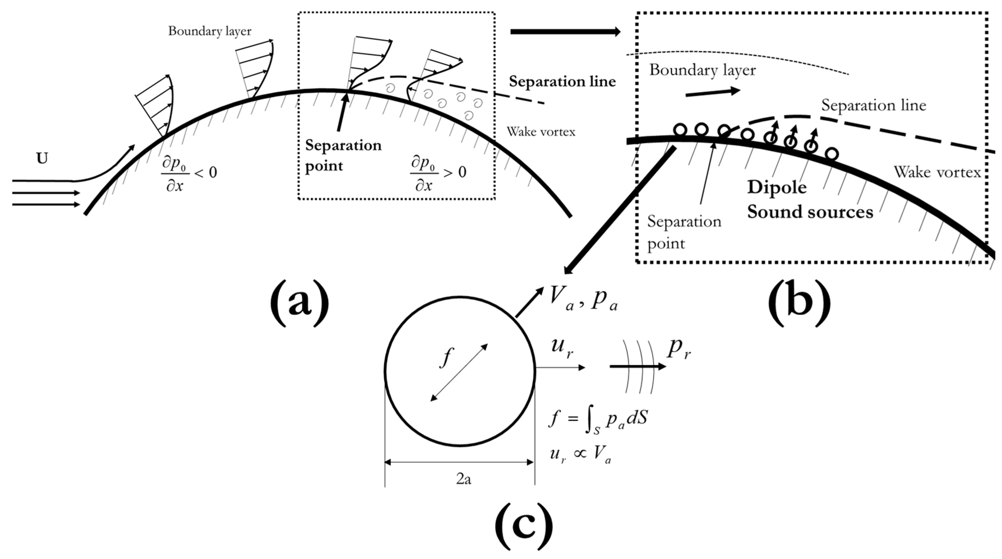
2.1. Basic Idea

The interaction of high-speed moving objects with the fluid produces a complex flow field. This phenomenon can be regarded as a typical flow state on a curved surface, as shown in Figure 1a. The fluid flows along the curved surface, producing a boundary layer, combined with strong pressure fluctuations. In the adverse pressure gradient area, fluid separation occurs, and the pressure fluctuation is more intense. In this process, the oscillating force of the wall to the fluid in the boundary layer produces aerodynamic sound dipole sources, which exist near the wall [5,6,7], as shown in the dotted box part in Figure 1a,b. It is assumed that the sound source on the surface is composed of numerous small aerodynamic sound sources, and each source radiates sound energy outward, as shown in Figure 1c. In Figure 1, $U$ is the inflow velocity; $p_0$ is the flow field pressure; $f$ is the oscillating force acting on the dipole source; $V_a$ is the oscillating velocity of the dipole source; $p_a$ is the sound pressure on the boundary of the spherical source; $p_r$ is the sound pressure radiated in space; $u_r$ is the radial velocity on the boundary of the spherical source; and $a$ is the radius of the sphere.

In order to describe the characteristics of the sound source in Figure 1b and realize the identification of the sound dipole source in the near-wall region, this paper first obtains the sound pressure radiated from a single spherical source in Figure 1c, which is based on the Lighthill sound propagation equation. Secondly, according to the FW-H equation in which the sound dipole source is an oscillating force source, by using the relationship between the total radiated sound pressure of a single source on its boundary surface when the oscillating force is equal and the radial oscillating velocity is continuous, the relationship between the sound pressure of a single source radiation $p_a$ and $V_a$ and the oscillating force $f$ is obtained, so as to obtain the relationship between the sound intensity of the source and the oscillating force of the flow field. Finally, the relationship between the intensity and sound power of a single sound dipole source and the pressure gradient at the corresponding location in the flow field is obtained using the knowledge of hydrodynamics that the oscillating force $f$ is related to the pressure gradient in the flow field [9]. This relationship is applicable to other dipole sources. The pressure gradient at any location in the flow field can be obtained by computational fluid dynamics, and the relationship between the sound source intensity and the pressure gradient can be used to describe the location and sound power of the sound dipole sources near the wall. Thus, the identification of aerodynamic sound dipole sources is achieved.

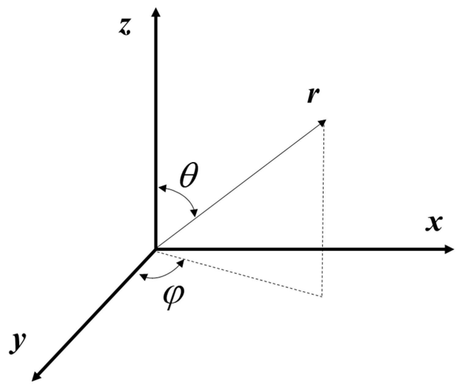
2.2. Formula Derivation

The study object applied here is the terrestrial vehicle. It can therefore be considered an incompressible, isentropic problem. It is assumed that the sound dipole source is composed of multiple micro-spherical sound sources. The source is an oscillating spherical source that repeats the linear vibration near the equilibrium location, causing the expansion and contraction of the local fluid and thereby radiating sound energy outward. A spherical coordinate system is shown in Figure 2. If only the vibration in the z-axis direction is considered and the sound field does not change with the azimuth angle φ, then the sound wave propagation equation can be simplified as follows:

$$\frac{1}{c_0^2}\frac{{\partial }^{2}p}{\partial t^2}-\frac{1}{r^2}\frac{\partial p}{\partial r}(r^2\frac{\partial p}{\partial r})-\frac{1}{r^2\sin \theta }\frac{\partial }{\partial \theta }(\sin \theta \frac{\partial p}{\partial \theta })=0,$$

(4)

where $p$ is the sound pressure; $c_0$ is the speed of sound, $r$ is the distance the sound wave travels; $t$ is the time of sound propagation; and $\theta ,\phi$ are the elevation and azimuth angles in the spherical coordinate system ($0\le \theta \le \pi ,0\le \phi \le 2\pi$).

Assuming that the spherical source performs simple harmonic vibration along the z-axis, the vibration velocity is $v(t)=V_a{e}^{i\omega t}$, $a$ is the radius of the sphere, $\omega$ is the angular frequency. Its radial component velocity is then defined as $u_r(a,\theta ,t)=V_a\cos \theta e^{i\omega t}$, and the solution to Equation (4) is:

$$p(r,\theta ,t)=i{\rho }_0{c}_{0}k{a}^3{V}_a\frac{\sqrt{1+{(kr)}^2}}{r^2\sqrt{4+{(ka)}^4}}\cos \theta *\exp (i*\left[\omega t-k(r-a)+\arctan (kr)-\arctan (\frac{2ka}{2-{(ka)}^2})\right]),$$

(5)

where ${\rho }_0$ is the air density,

The vibration velocities of the particles at the directions of the three coordinate axes are:

$$u_r(r,\theta ,t)=a^3{V}_a\frac{\sqrt{4+{(kr)}^2}}{r^3\sqrt{4+{(ka)}^4}}\cos \theta *\exp (i*\left[\omega t-k(r-a)+\arctan (\frac{2kr}{2-{(kr)}^2})-\arctan (\frac{2ka}{2-{(ka)}^2})\right]),$$

(6)

$$u_{\theta }(r,\theta ,t)=a^3{V}_a\frac{\sqrt{1+{(kr)}^2}}{r^3\sqrt{4+{(ka)}^4}}\sin \theta *\exp (i*\left[\omega t-k(r-a)+\arctan (kr)-\arctan (\frac{2ka}{2-{(ka)}^2})\right]),$$

(7)

$$u_{\phi }(r,\theta ,t)=0.$$

(8)

The corresponding sound intensity can be obtained as:

$$I_r=\frac{9f_{}^2{\cos }^2\theta }{32{\pi }^2{\rho }_0{c}_0^3}\frac{{\omega }^2}{r^2}\frac{1}{\sqrt{1+{(ka)}^2}},$$

(9)

$$I_{\theta }=I_{\phi }=0.$$

(10)

For the surface of the spherical source, $r=a\to 0$. Equations (5) and (6) become:

$$p(r,\theta ,t)=\frac{3f\cos \theta }{4\pi r^2}\exp (i\omega t),$$

(11)

$$u_r(r,\theta ,t)=\frac{3\cos \theta }{2\pi {\rho }_0{r}^3}{\displaystyle \int f\exp (i\omega t)dt}.$$

(12)

The above is the case of the vibration at one single-frequency, for the oscillating sources there exists force $F$, $F=f\exp (i\omega t)$, then:

$$p(a,\theta ,t)=\frac{3F\cos \theta }{4\pi a^2},$$

(13)

$$u_r(a,\theta ,t)=\frac{3\cos \theta }{2\pi {\rho }_0{a}^3}{\displaystyle \int Fdt}.$$

(14)

The sound intensity of the oscillating source vibrating in one direction is:

$$I_r=\frac{1}{T}{\displaystyle {\int }_0^T(\frac{3F\cos \theta }{4\pi a^2}\frac{3\cos \theta }{2\pi {\rho }_0{a}^3}{\displaystyle \int F}dt)dt}=\frac{9{\cos }^2\theta }{8{\pi }^2{\rho }_0{a}^5}\frac{1}{T}{\displaystyle {\int }_0^T(F{\displaystyle \int F}dt)dt},$$

(15)

$$I_{\theta }=I_{\phi }=0.$$

(16)

Integrate the sound intensity over the sphere to get the sound power of the sound source on the sphere:

$$\mathsf{\Pi }={\displaystyle \int I_r}dS=\frac{3}{2\pi {\rho }_0{a}^3}\frac{1}{T}{\displaystyle {\int }_0^T(F{\displaystyle \int F}dt)dt}.$$

(17)

Equation (17) represents the sound power radiated by each micro-element in the turbulent field. The computational fluid dynamics method can calculate the oscillating force in the equation, and the dipole sound intensity and sound power can be obtained to realize the identification of the sound dipole source.

In Equation (17) the oscillating force $F$ is the oscillating amount of the force vector acting on a point location in the fluid, and the sound pressure wave equation of the force point source in the flow field can be expressed as:

$$\frac{1}{c_0}\frac{{\partial }^{2}p}{\partial t^2}-\nabla ·(\nabla p)=-\nabla ·\mathit{f}.$$

(18)

The instantaneous force is $\mathit{f}=\nabla p_0+\nabla \times {\mathit{u}}_0$, where $p_0$ is the pressure of the flow field and ${\mathit{u}}_0$ is the velocity vector of the flow field [9]. Its fluctuation is ${\mathit{f}}_{flu}=\nabla p_{0,flu}+\nabla \times {\mathit{u}}_{0,flu}$, the subscript flu represents the oscillating value, and substituting it into Equation (18) can obtain $\nabla ·(\nabla \times {\mathit{u}}_{0,flu})=0$, the part related to the velocity vector does not contribute to the sound field. Thus, ${\mathit{f}}_{flu}=\nabla p_{0,flu}$.

Then Equation (14) can calculate the sound power at each location:

$$\mathsf{\Pi }={\displaystyle \int I_r}dS=\frac{3}{2\pi {\rho }_0{a}^3}\frac{1}{T}{\displaystyle {\int }_0^T(F{\displaystyle \int F}dt)dt}=\frac{3}{2\pi {\rho }_0{a}^3}\frac{{\displaystyle {\sum }_{j=1}^N{\left|\nabla p\right|}_{0,flu,j}^2\times (\Delta t)}}{N}.$$

(19)

To use numerical computation for simulation, the formula is expressed in the form of discrete time steps, where ${\left|\nabla p\right|}_{0,flu,j}$ is the pressure of the flow field at each time step; $N$ is the total number of time steps; $\Delta t$ is the time interval.

Considering the vibration direction is not consistent for any single spherical source, the vibration in any direction can be decomposed into three axes in the Cartesian coordinate system:

$${\mathit{f}}_{rand}=f_x{e}^{i\omega t}{\mathit{e}}_x+f_y{e}^{i\omega t}{\mathit{e}}_y+f_z{e}^{i\omega t}{\mathit{e}}_z,$$

(20)

where ${\mathit{f}}_{rand}$ is the oscillating force vector of a single spherical source; $f_x,f_y,f_z$ is the magnitude at the three coordinate axes; ${\mathit{e}}_x,{\mathit{e}}_y,{\mathit{e}}_z$ are the unit vectors at the three axes.

The total sound power is the superposition of the sound power components at each axis is:

$${\mathsf{\Pi }}_{total}={\mathsf{\Pi }}_x+{\mathsf{\Pi }}_y+{\mathsf{\Pi }}_z=\frac{3}{2\pi {\rho }_0{a}^3}\frac{{\displaystyle {\sum }_{j=1}^N{\left|\nabla p\right|}_{0,flu,j,total}^2\times (\Delta t)}}{N},$$

(21)

where ${\left|\nabla p\right|}_{0,flu,j,total}^2={\left|\nabla p\right|}_{0,flu,j,x}^2+{\left|\nabla p\right|}_{0,flu,j,y}^2+{\left|\nabla p\right|}_{0,flu,j,z}^2$, ${\left|\nabla p\right|}_{0,flu,j,x},{\left|\nabla p\right|}_{0,flu,j,y},{\left|\nabla p\right|}_{0,flu,j,z}$ are the components at each axis.

3. Discussion on the Effectiveness of Sound Source Simulation Method Based on Cylindrical Flow

To illustrate the effectiveness of the sound source simulation method proposed in this paper, the specific typical sound dipole source characteristics of the flow around the cylinder are considered here. On the one hand, the descriptive effect of the above method on the sound source is presented, and, on the other hand, compared with the APE method, this proposed method is shown to be more reliable.

3.1. Verification of the Numerical Simulation Methods

In Equation (21), it is necessary to accurately calculate the fluctuating pressure gradient at each time step in the flow field. The sound pressure in the far-field radiated by a circular cylinder is predicted by this numerical method, and the reliability of the aerodynamic numerical simulation method is verified compared with the wind tunnel test results.

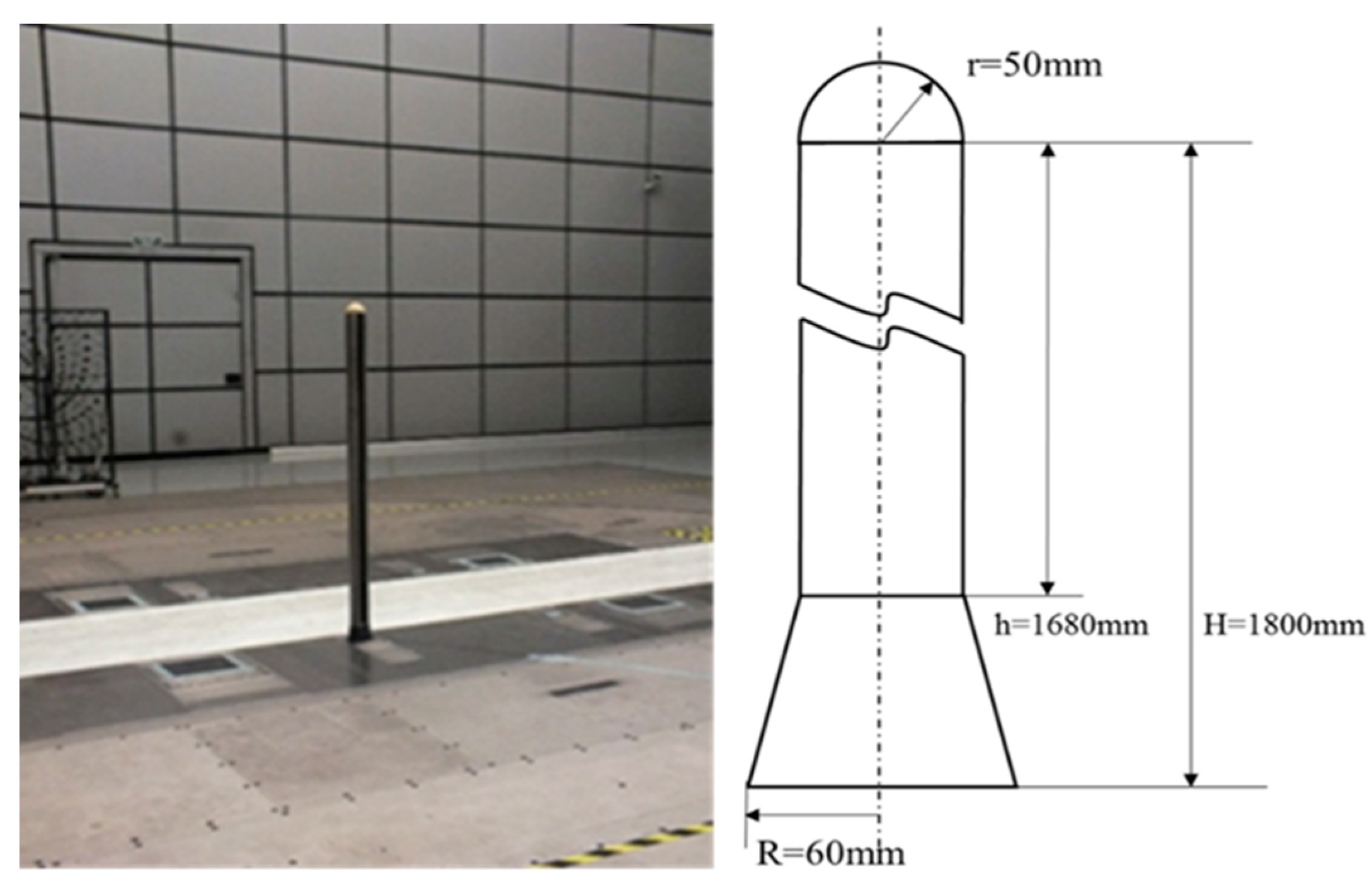
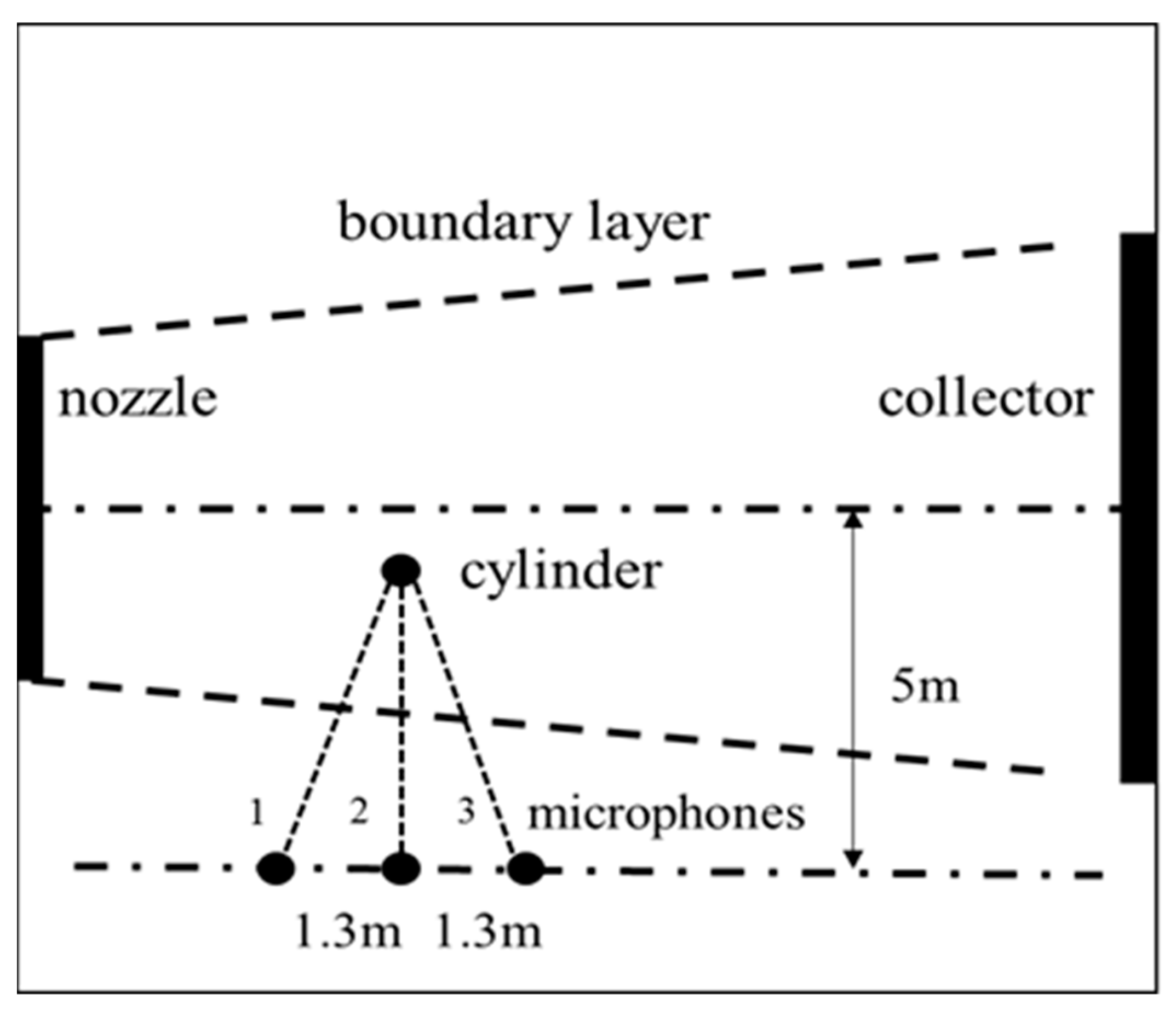
3.1.1. Experiments in the Wind tunnel

The experiment was conducted at the aeroacoustics wind tunnel in the Shanghai Automotive Wind Tunnel Center of Tongji University. The size of the test section is 22 m × 17 m × 12 m, the nozzle is 4.25 m high and 6.5 m wide, and the maximum wind speed is 250 km/h. The acoustic properties of a smooth, rigid cylinder with a height of 1.8 m and a diameter of 0.1 m were studied, as shown in Figure 3. The bottom of the cylinder is a circular truncated cone, and the top is a hemisphere to reduce the aerodynamic noise caused by the flow at the root and free end at the top, highlighting the noise characteristics generated by the quasi-two-dimensional flow around the cylinder.

Figure 4 shows the locations of the microphones and the cylinder. Specifically, three equally spaced microphones were used to measure far-field sound pressure at a location parallel to the jet centerline outside the jet shear layer of the nozzle. The microphones are located 1.2 m above the ground, 5 m from the mid-plane of the flow field, and 4.45 m from the center of the cylinder; the distance between each microphone is 1.3 m. The wind speed out of the nozzle during the test was 80 km/h. The microphones used in the test are free-field microphones from GRAS, Denmark, and the data acquisition and analysis equipment used in the SQLABIII multi-channel acquisition and analysis system are from HEAD Acoustics, Germany.

The uncertainty of this experiment is primarily attributed to the background noise of the wind tunnel, the nozzle wind speed, and the error of the measurement equipment. The effect of environmental parameters such as temperature, air pressure, and air density over a short period of time can be ignored. In the experiment, the sound pressure level at the measuring point was measured at a wind speed of 80 km/h with and without the cylinder. At the vortex shedding frequency of the cylinder, the noise generated by the cylinder was 69.7 dB (A), while it was 45.0 dB (A) without the cylinder. The difference of 24.7 dB (A) indicates that the influence of background noise on the measurement results can be neglected. Additionally, four repeated measurements of the sound pressure levels at three measurement points at a wind speed of 80 km/h were conducted, and the results showed errors ranging from 0.02 to 0.04 dB (A), indicating that the influence of wind speed changes at the wind tunnel nozzle and measurement equipment errors is minimal. The experimental results are therefore reliable.

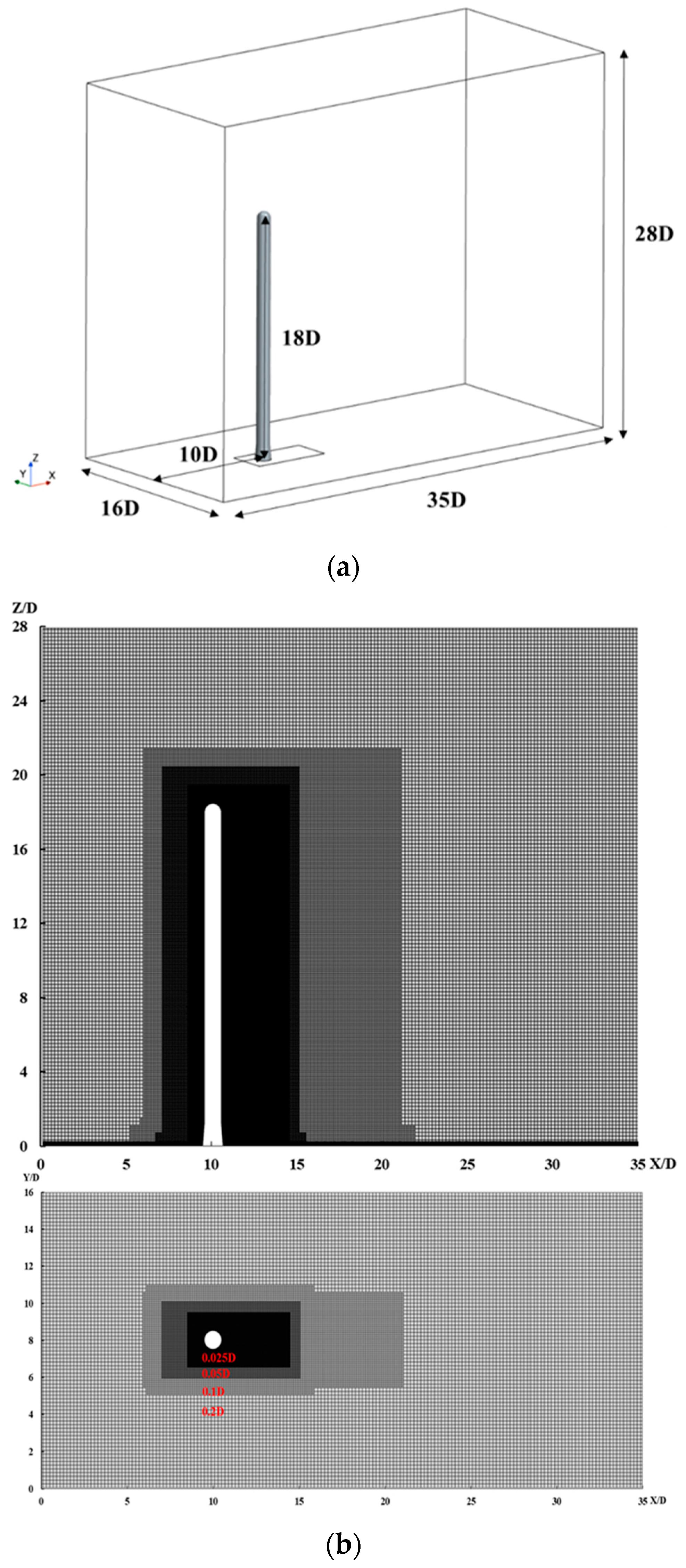
3.1.2. Numerical Simulation Model

To be comparable, the simulation setting is consistent with the experimental situation. The details of the modelling are shown in Figure 5a. The diameter D of the cylinder is 0.1 m and the height is 18D. The size of the computational domain is set to 35D × 16D × 28D, the center of the cylinder is 10D away from the inlet section and 8D away from the walls on both sides to ensure that the inlet flow, both sides, and the top are not affected by the boundary. Three sound pressure measurement points are set as shown in Figure 4, and the far-field noise generated by the cylindrical surface at the measurement point is calculated using the FW-H equation for comparison with experimental results.

Star-CCM+ is used for mesh generation and simulation. The size of the surface grid is 0.025D, and the top part of the cylinder is an unstructured grid, while the rest is a structured grid. The cylindrical grid is a hexahedral grid with three refinement regions. The outermost grid size is 0.02D, and the three refinement regions have grid sizes of 0.1D, 0.05D, and 0.025D, respectively, as shown in Figure 5b. The boundary layer grid on the cylinder surface adopts the O-grid strategy. The first layer of grid thickness is 0.0001D, the boundary layer growth rate is 1.2, and the number of boundary layers is 31 to ensure that y⁺ < 1. The total number of grids is approximately 32 million.

A series of numerical simulations were conducted by further refining the grid and reducing the time step. The results are shown in

Table 1. Grid sensitivity verification.

No.	Total Number of Grids/Million	Minimum Time Step/S	Peak Frequency/Hz	Sound Pressure Level/dB
1	32	2 × 10−3	44.92	67.3
2	34	2 × 10−3	46.88	67.6
3	36	2 × 10−3	46.88	66.4
4	40	2 × 10−3	48.83	65.5
5	40	1 × 10−3	48.83	66.8
6	44.6	2 × 10−3	48.82	65.5

, where No. 1 is the initial grid. It shows that as the grid is further refined, the time step is further reduced, the differences in total sound pressure level are within 2.1 dB, and the shift in the peak frequency is within 4 Hz.

The inlet velocity of the computational domain is 80 km/h, and the Reynolds number is about Re = 1.48 × 10⁵. It is set up as an incompressible fluid. The top side and two sides of the computational domain are set as symmetric boundary conditions, and the remaining surfaces are no-slip wall boundaries. The boundary conditions in the computation are shown in

Table 2. Boundary conditions for simulation.

Computational Domain Boundaries	Boundary Condition Type
Inlet	Velocity inlet, v = 80 km/h
	The turbulence intensity: 1%
	The turbulent viscosity ratio: 10
Outlet	Pressure outlet, gauge pressure: 0
	The turbulence intensity: 1%
	The turbulent viscosity ratio: 10
Cylinder and ground	No-slip wall

.

Firstly, the SST (Menter) K-Omega model is applied in the steady flow simulation calculation. Then use the LES (Large Eddy Simulation) for unsteady simulation, and the sub-grid-scale model is the WALL Subgrid-scale model. The SST k-Omega equation considers the transfer of turbulent shear stress and can predict boundary layer flow with an adverse pressure gradient [31]. The transfer equation for the turbulent energy dissipation rate $w$ is as follows:

$$\frac{\partial }{\partial t}(\rho w)+\frac{\partial }{\partial x_j}(\rho w{u}_j)=\frac{\partial }{\partial x_j}({\mathsf{\Gamma }}_w\frac{\partial w}{\partial x_j})+G_w-Y_w+D_w+S_w,$$

(22)

where $t$ is time; $\rho$ is the density of air; ${\mathsf{\Gamma }}_w$ is the effective diffusion coefficient of $w$; $G_w$ is the production term; $Y_w$ is the dissipation term; $D_w$ is the cross diffusion term; $S_w$ is the user-defined term.

The equation for LES is obtained by filtering the Navier-Stokes equation in the wavenumber domain or spatial domain, filtering out vortices smaller than the filter width, and obtaining the governing equation for large vortices. The variables with an underline in the equation are the filtered field variables [32]:

$$\frac{\partial \rho }{\partial t}+u\frac{\partial \rho {\overline{u}}_i}{\partial t}=0,$$

(23)

$$\frac{\partial \rho {\overline{u}}_i}{\partial t}+\frac{\partial \rho \overline{u_i{u}_j}}{\partial x_j}=\frac{\partial }{\partial x_j}(\mu \frac{\partial {\overline{u}}_i}{\partial x_j})-\frac{\partial \overline{p}}{\partial x_j}-\frac{\partial {\tau }_{ij}}{\partial x_j},$$

(24)

where ${\tau }_{ij}=\rho \overline{u_i{u}_j}-\rho {\overline{u}}_i·{\overline{u}}_j$ is the sub-grid-scale stress, and can be expressed as:

$${\tau }_{ij}=2{\mu }_t\overrightarrow{\mathit{S}}-\frac{2}{3}({\mu }_t\nabla ·{\overline{u}}_i+\rho \kappa )\overrightarrow{\mathit{I}},$$

(25)

where $\overrightarrow{\mathit{S}}$ is the stain rate tensor; $\kappa$ is the sub-grid-scale turbulent kinetic energy; $\overrightarrow{\mathit{I}}$ is the unit tensor; ${\mu }_t$ is the sub-grid-scale turbulent viscosity in the WALL Subgrid-scale model [33]:

$${\mu }_t=\rho {\Delta }^2{S}_{\mathrm{s}h},$$

(26)

where $\Delta$ is the length scale or grid filter width; $S_{sh}$ is the deformation parameters.

The time step is set at 5 × 10⁻³ s at the beginning. After 1 s of physical time, the stabilized results are obtained, and then the time step is changed to 2 × 10⁻³ s and the simulation continues for 3.2 s of physical time.

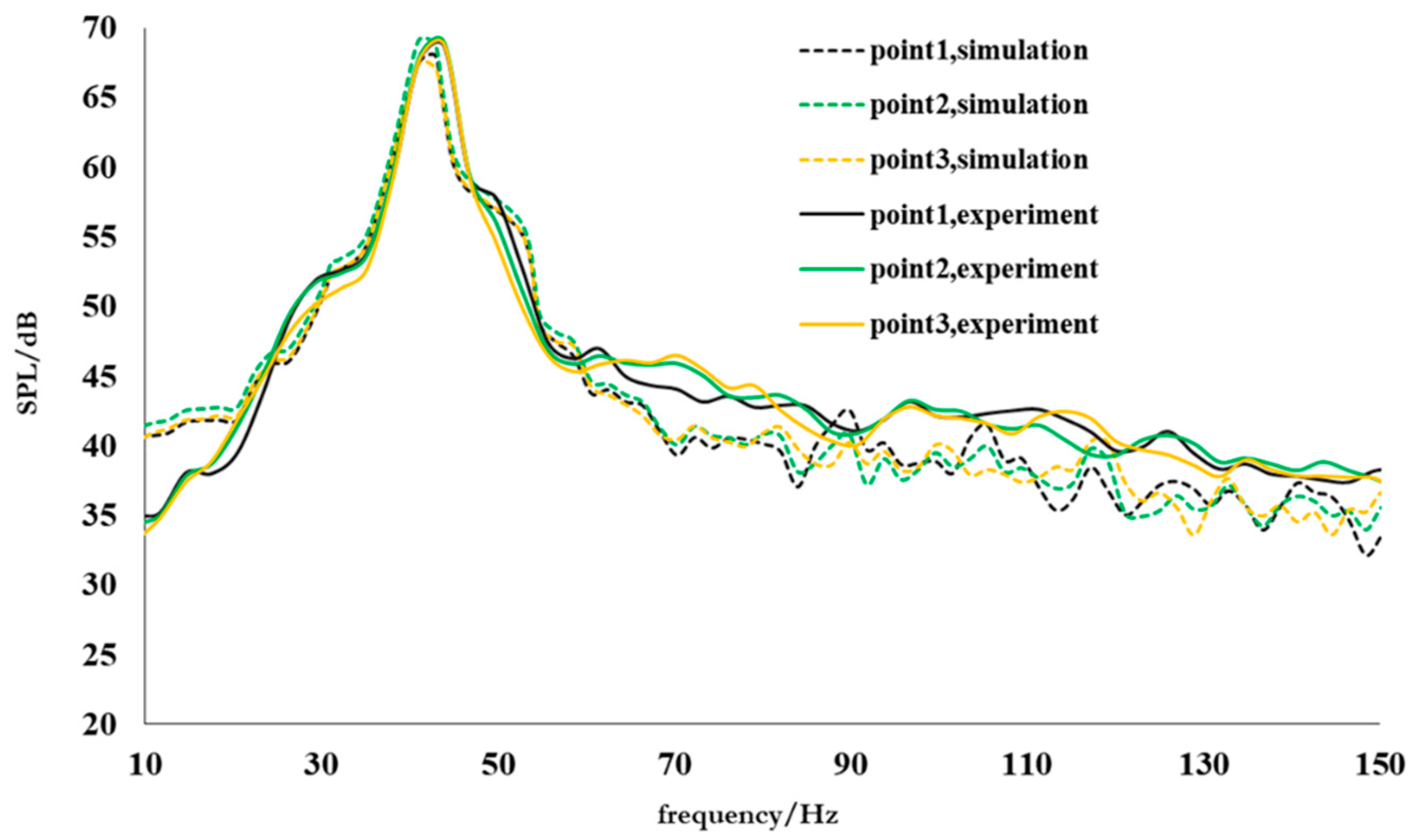
3.1.3. Comparison of Simulation and Experimental Results

Figure 6 shows the comparison of the sound pressure level between the measured results at the three points and the corresponding simulation calculation. It shows that both curves are relatively consistent. The simulations can show the prominent sound pressure peak of the flow around the cylinder at the vortex shedding frequency. Therefore, this calculation can meet the needs of further research.

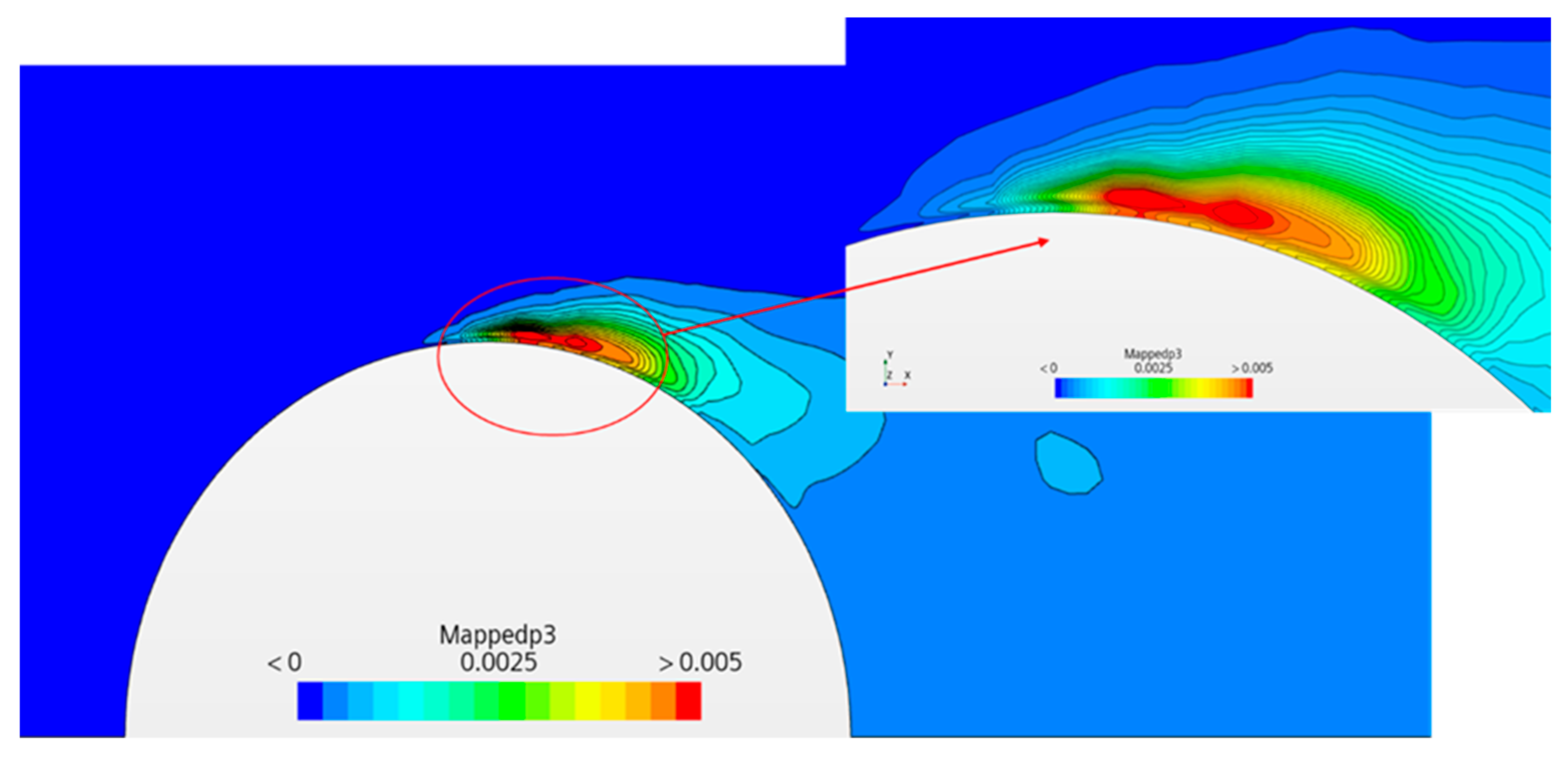
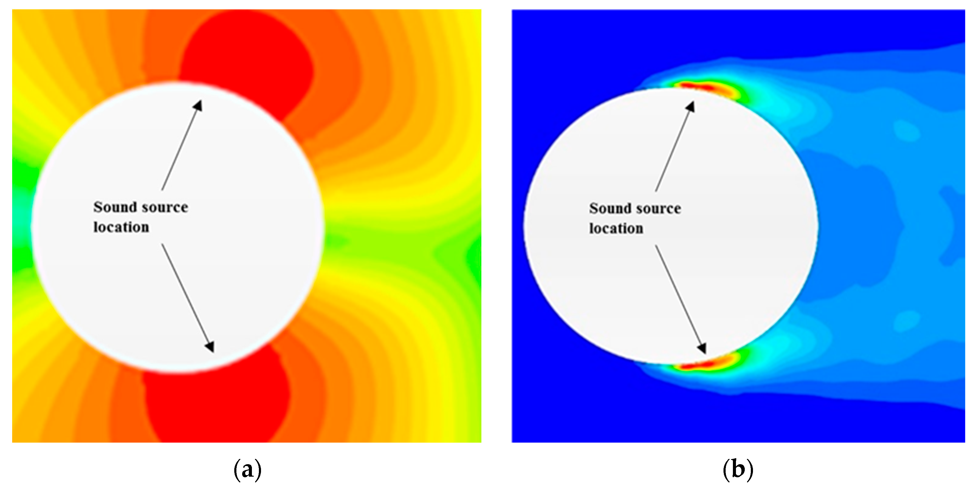
3.2. Sound Dipole Source of the Flow around a Cylinder

${\left|\nabla p\right|}_{0,flu,j,total}$ at each point around the cylinder can be obtained by the CFD and is then substituted into Equation (21) to obtain the dipole source distribution of the flow around the cylinder, as shown in Figure 7. The time-averaged results of the sound power of the dipole source are shown, and the red region reflects the dipole source.

It can be clearly seen from Figure 7 that the sound dipole source is distributed in the adverse pressure gradient area and has a certain volume size. Its radial thickness is about 3 mm, and its circumferential length is about 10 mm. The location of the maximum sound source intensity is not on the wall but is 1 mm away from the wall. Based on the analysis in Section 4, it can be seen that the sound source area is located in the fluid separation area, which is the sound dipole source due to the large pressure fluctuation generated by the fluid separation, which is consistent with the previous research results. It can be seen from the results that this method clearly shows sound power and detailed distribution characteristics, which are rare in the existing methods. Therefore, this is a new method to identify the sound dipole source.

It can be seen from Figure 7 that the sound dipole source distribution is not the surface sound source distribution proposed in the references but the volume sound source. This will be discussed in Section 4.

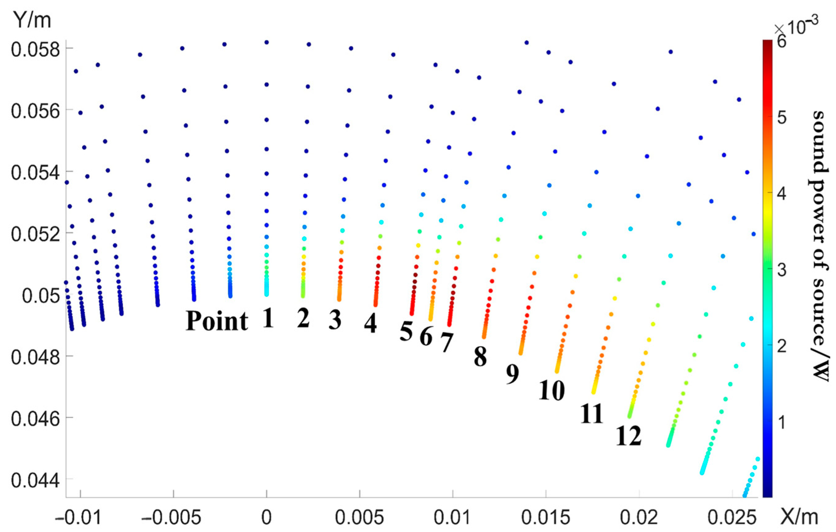
3.3. Verification of the Distribution of Sound Dipole Sources

The APE method can be used to calculate the sound radiation from the sound source. The sound pressure amplitude becomes larger as it is closer to the position of the actual sound source, which can reveal the location of the sound source. To verify the accuracy of the dipole source distribution obtained by the proposed method, the APE method is also used here to calculate the near-field sound around a circular cylinder [12].

The sound pressure level of the same cylinder model as that in Figure 5 is predicted by the APE method and also compared with those obtained by the current method, as shown in Figure 8. It can be seen from Figure 8 that the locations of the sound source revealed by two methods are approximately the same, which indicates the accuracy of the sound dipole source distribution in this study. In addition, the location of the sound source and the sound power seem clearer with this method.

4. Discussion

This section discusses the sound dipole source obtained in this study from the perspective of the relationship between the sound phenomenon and the flow field, such as the separation and vortex shedding of the flow around a cylinder and the correlation between the sound dipole source location and the flow field.

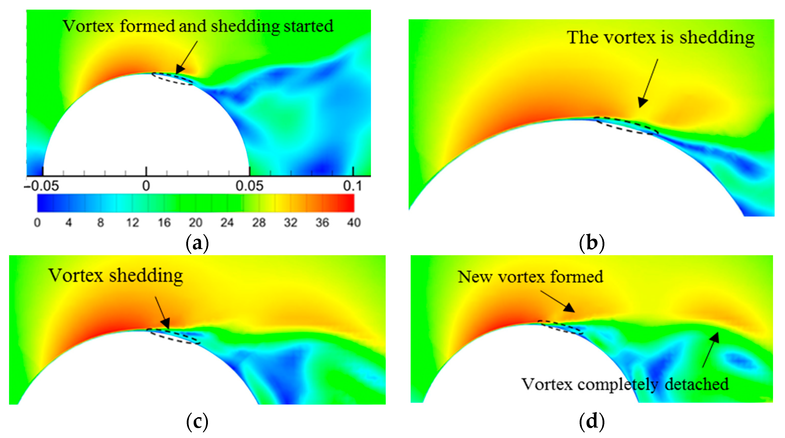
4.1. The Relationship between the Sound Source and the Vortex Shedding

The oscillating force acting on the fluid by the wall induces the sound dipole source. During the vortex shedding process of the flow around the cylinder, the interaction between the fluid and the cylinder wall is relatively intense. Figure 9 is the contour plot of the velocity field at different times of the flow around the cylinder, which characterizes the process of vortex formation and shedding. Specifically, Figure 9a indicates the initial stage of the vortex and its shedding, which occurs in the front region of the incoming flow, and its formation is located in the front of the sound dipole source region (the dotted line in the figure). Figure 9b indicates the backward location of the vortex shedding, corresponding to the backward area of the sound dipole source. Figure 9c shows that the vortex shedding location moves further backward and the shedding process is close to completion. The wake area expands, and the shedding location is far away from the sound source location, indicating that the effect of this shedding process on the wall is weakened and the sound dipole source effect is also weakened. Therefore, the sound dipole source disappears in the rear area of the cylindrical wall. Figure 9d shows that the vortex falls off completely, while the new vortex forms and starts to fall off gradually after the separation point, which repeats the above process. The fluid velocity change and momentum exchange are intense, and the oscillating force is stronger near the wall, which is the main causality for the formation of the sound dipole source and its regional distribution.

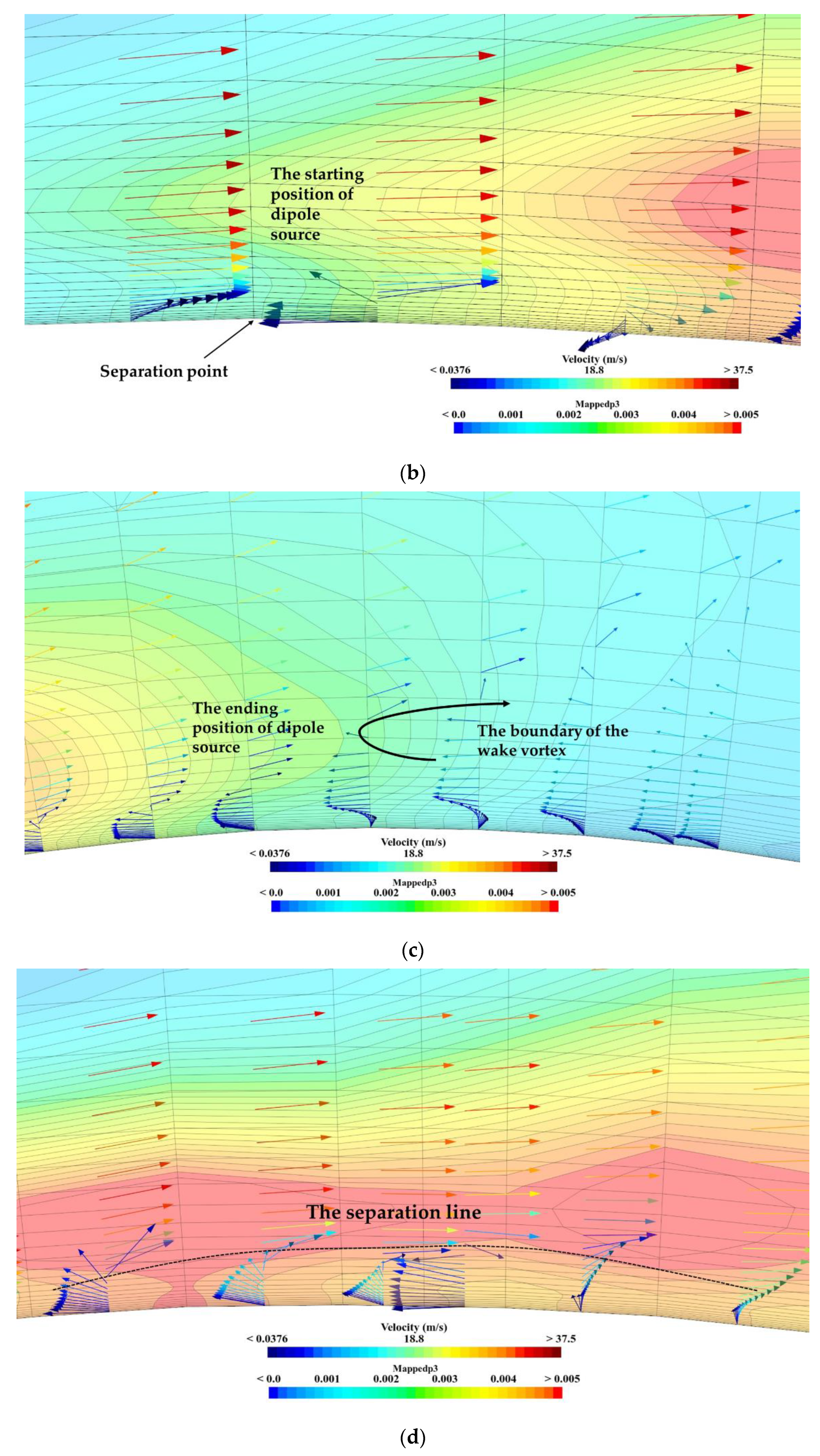
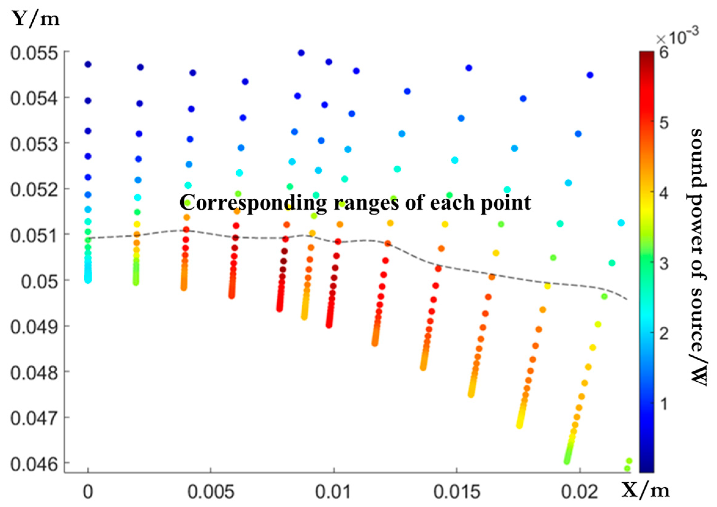
4.2. The Relationship between the Sound Source Area and the Separation Area

The time-averaged velocity vector field is compared with the sound power distribution of the sound dipole source, as shown in Figure 10a, where the contour plot is the sound dipole source distribution, and the vector is the velocity distribution. In particular, Figure 10b indicates that the starting location of the sound dipole source area is basically coincident with the starting location of the separation, whereas Figure 10c indicates the ending location is basically similar to the location where the separation flow completely leaves the wall area, that is, the location where the wake vortex is generated. The intensity of the dipole source is not large on the wall, and Figure 10d indicates that the location of the maximum intensity starts from the separation line and ends near the boundary of the boundary layer along the wall normal.

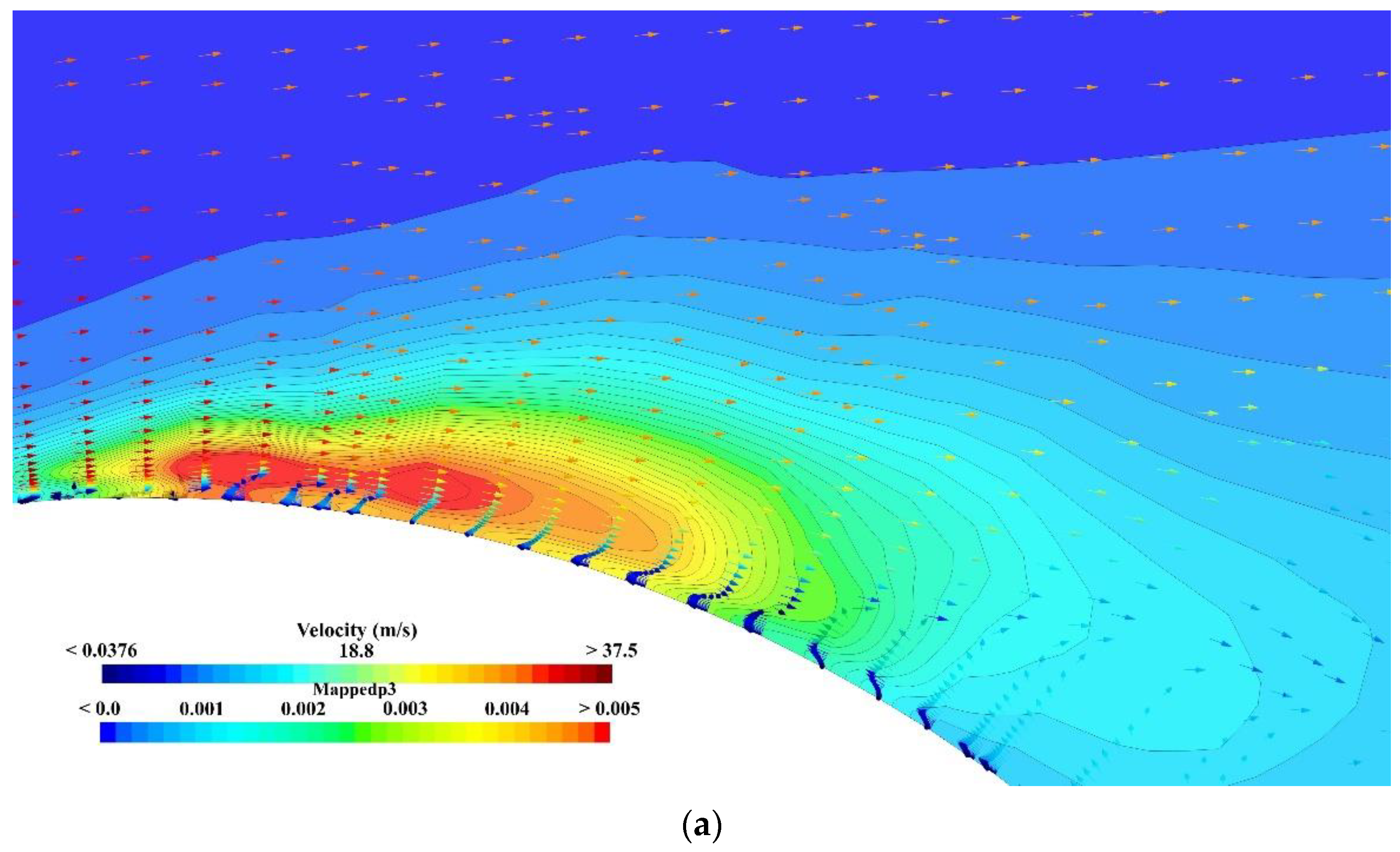
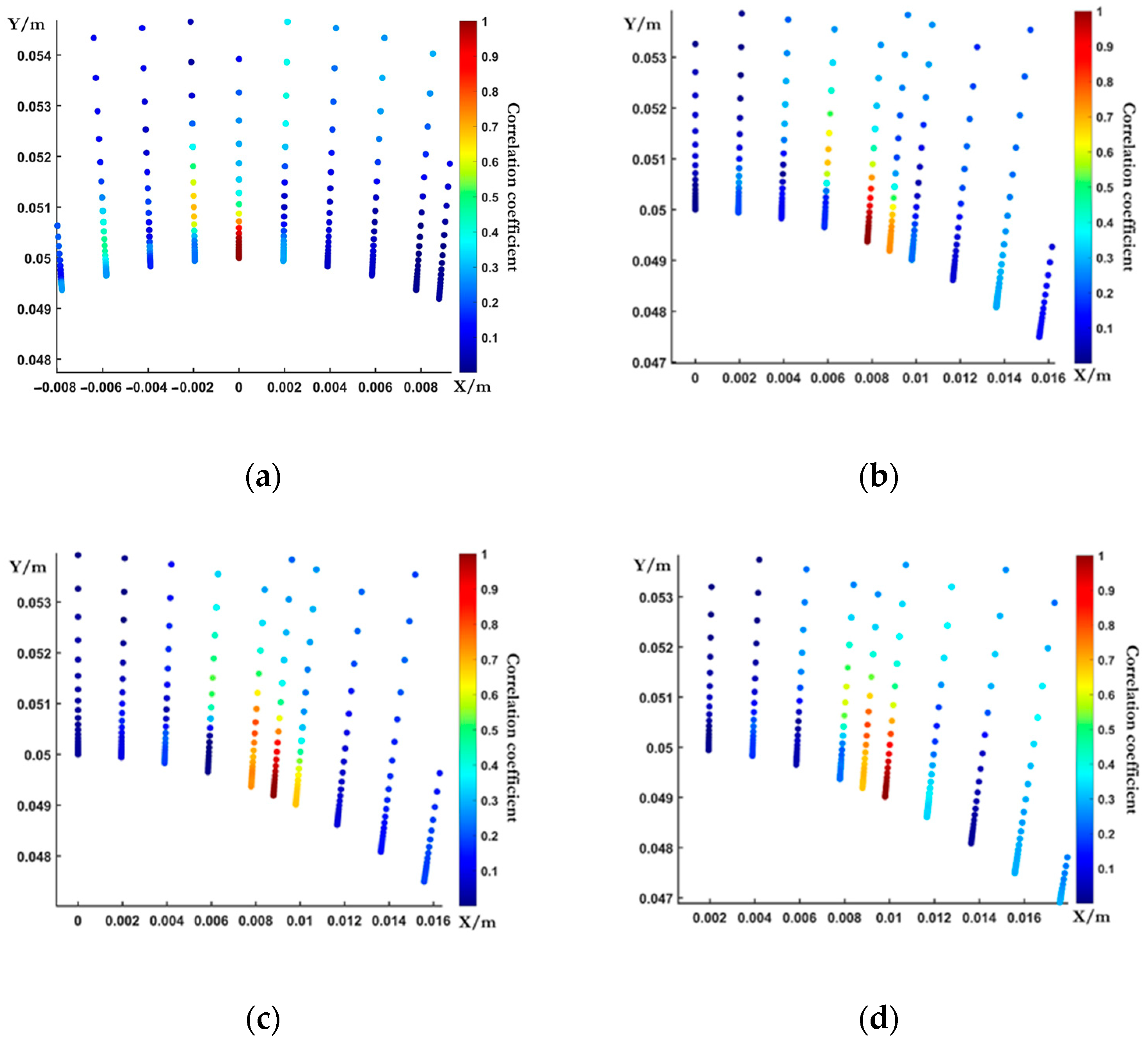
4.3. Correlation between the Sound Source and the Flow Flied

From the above analysis, it can be seen that the sound dipole source does not always present characteristics of the surface distribution but has a thickness attached to the wall. Since the essence of the sound dipole source is the effect of the wall on the nearby flow field, it is therefore necessary to carry out a correlation analysis of the sound power of the wall point and the space point in the sound source region to study the influence of the wall on the fluid and further analyze the area where the sound dipole source exists. Figure 11 shows the distribution of the sound power of the sound dipole source in space by displaying the contour plot as a scatter plot.

In all the spatial separation points, the data points 1–12 on the wall are selected in turn, as shown in Figure 11. A few representative points are selected, and their correlation coefficients with all the other points are shown in Figure 12. The correlation coefficient of each point itself is 1, which is the red area in Figure 12. It can be seen that each wall point has a strong correlation with the nearest point along the radius direction and its adjacent points, but a weak correlation with other points. This indicates that the sound dipole source generated by the force effect of the wall on the fluid is generated not only on the wall but also in space and has a stronger correlation along the radius direction. There is a correlation between the wall point and the upstream point, indicating that the forward flow (turbulence after the separation point) has a certain effect on the wall, and it is also an important reason for the formation of the wall force effect. Therefore, the sound dipole source is the result of the combined effect of the separation of airflow and the cylindrical wall. The force source is the wall and affects a certain area of the space.

The range of correlation coefficients greater than 0.5 in the radial direction of each point on the above-mentioned wall surface indicates a strong correlation, which is considered to be the range of the oscillating force acting in the radial direction of the wall surface. Connect the corresponding ranges of each point into a line, as shown by the dotted line in Figure 13 and it indicates that the distribution range of the dipole source is approximately the same as that of the wall surface force effect.

In summary, the aerodynamic sound dipole source exists in a specific turbulent region attached to the wall. It starts at the separation point along the circumferential direction of the wall surface and finishes at the starting location of complete vortex shedding and wake vortex formation. There is a certain thickness along the radial direction, which gradually increases backward.

5. Conclusions

The near-wall flow field formed by the interaction between the fluid and the rigid wall surface is taken as the research object in this paper. Taking into account the aerodynamic sound dipole source generated by the oscillating force in the flow field, the relationship between the fluctuation source and its sound radiation and the relationship between the oscillating force and the pressure gradient of the flow in the near-wall flow field are studied, and a new identification method of the sound source is obtained. The formula for calculating the sound power of the aerodynamic dipole source generated by the flow around the wall is derived, and the proportional relationship between the sound power of the aerodynamic sound dipole source and the square of the oscillating force or the square of the pressure gradient in the flow field is presented. Combining this formula with the CFD method, the identification of the aerodynamic dipole source flowing around the wall of the object can be implemented.

The application to the sound source identification of the flow around a cylinder shows that the proposed method can offer the sound power and detailed distribution of the sound dipole source. It is a method to describe the sound source from a new perspective.

By analyzing the identification results of the sound dipole source, the relationship between the sound source and the separation and vortex shedding, and their corresponding correlation analysis, it is found that the aerodynamic sound dipole source is not the surface distribution considered by the existing research but the volume distribution. It exists in an unstable flow region attached to the wall, and its starting point is located at the separation point along the circumferential direction of the wall, which terminates at the location where the complete vortex falls off and the trailing vortex forms. There is a thickness along the radial direction, and the thickness gradually increases backward. This identification method is useful to further discover the characteristics of the sound dipole source and to deepen the understanding of this sound source.

References

1. Watkins, S. Aerodynamic noise and its refinement in vehicles. In Vehicle Noise and Vibration Refinement; Woodhead Publishing Limited: Southton, UK, 2010; Volume 48, pp. 219–234. [Google Scholar]
2. Khalighi, Y. Computational Aeroacoustics of Complex Flows at Low Mach Number; Stanford University: Stanford, CA, USA, 2010. [Google Scholar]
3. Hucho, W.H. The Aerodynamic Drag of Cars. In Aerodynamic Drag Mechanisms of Bluff Bodies and Road Vehicles; Plenum: New York, NY, USA, 1978; pp. 1–44. [Google Scholar]
4. Watanabe, M.; Harita, M.; Hayashi, E. The Effect of Body Shape on Wind Noise. SAE Tech. Pap. 1978, 780266. [Google Scholar] [CrossRef]
5. Lighthill, M.J. On sound generated aerodynamically I, general theory. Proc. R. Soc. Lond. Ser. A 1952, 211, 564–587. [Google Scholar]
6. Curle, N. The influence of solid boundaries upon aerodynamic sound. Proc. R. Soc. Lond. Ser. A 1955, 231, 505–514. [Google Scholar]
7. Ffowcs Williams, J.E.; Hawkings, D.L. Sound generation by turbulence and surfaces in arbitrary motion. Philos. Trans. R. Soc. A 1969, 264, 321–342. [Google Scholar]
8. Brentner, K.S.; Farassat, F. Modeling aerodynamically generated sound of helicopter rotors. Prog. Aerosp. Sci. 2003, 39, 83–120. [Google Scholar] [CrossRef]
9. Zhang, Q. Fundamentals of Aeroacoustics; National Defense Industry Press: Beijing, China, 2012. [Google Scholar]
10. Casalino, D. An advanced time approach for sound analogy predictions. J. Sound Vib. 2003, 261, 583–612. [Google Scholar] [CrossRef]
11. Brentner, K.S.; Farassat, F. Analytical Comparison of the Sound Analogy and Kirchoff Formulation for Moving Surfaces. AIAA J. 1998, 36, 1379–1386. [Google Scholar] [CrossRef]
12. Ewert, R.; Schröder, W. Sound perturbation equations based on flow decomlocation via source filtering. J. Comput. Phys. 2003, 188, 365–398. [Google Scholar] [CrossRef]
13. Faßmann, B.W.; Rautmann, C.; Ewert, R.; Delfs, J.W. Prediction of porous trailing edge noise reduction via sound perturbation equations and volume averaging. In Proceedings of the 21th AIAA/CEAS Aeroacoustics Conference, Dallas, TX, USA, 22–26 June 2015; pp. 1–18. [Google Scholar]
14. Phillips, O.M. On the generation of sound by supersonic turbulent shear layers. J. Fluid Mech. 2006, 9, 1–28. [Google Scholar] [CrossRef]
15. Lilley, G.M. Appendix: Generation of Sound in a Mixing Region; Fourth Monthly Progress Report on Contact, F-33615-71-C-1663; U.S. Air Force Aeropropulsion Lab: Wright–Patterson AFB, OH, USA, 1972. [Google Scholar]
16. Howe, M.S. Theory of Vortex Sound; Cambridge University Press: Cambridge, UK, 2003. [Google Scholar]
17. Golstein, M.E. Turbulence generated by interaction of entropy with non-uniform mean flow. J. Fluid Mech. 1979, 93, 209–224. [Google Scholar] [CrossRef]
18. Golstein, M.E. The effect of finite turbulence spatial scale on application of turbulence by a contracting stream. J. Fluid Mech. 1980, 98, 473–508. [Google Scholar] [CrossRef]
19. Golstein, M.E. The coupling between flow instability and incident disturbance at a loading edge. J. Fluid Mech. 1981, 104, 217–246. [Google Scholar] [CrossRef]
20. Golstein, M.E. High frequency sound emission from moving point muhipole sources embeded in arbitrary transversely sheared mean flow. J. Sound Vib. 1982, 80, 499–521. [Google Scholar] [CrossRef]
21. Doak, P.E. Fluctuating Total Enthalpy as the Basic Generalized Sound Field. Theor. Comput. Fluid Dyn. 1998, 10, 115–133. [Google Scholar] [CrossRef]
22. Ribner, H.S. New Theory of Jet-Noise Generation, Directionality, and Spectra. J. Soundal Soc. Am. 1959, 31, 530–531. [Google Scholar] [CrossRef]
23. Powell, A. Theory of Vortex Sound. J. Acoust. Soc. Am. 1964, 36, 177–195. [Google Scholar] [CrossRef]
24. Mohring, W. A well posed acoustic analogy based on a moving acoustic medium. Physics 2010. [Google Scholar] [CrossRef]
25. Mao, Y.; Tang, H.; Xu, C. Vector Wave Equation of Aeroacoustics and Sound Velocity Formulations for Quadrupole Source. AIAA J. 2016, 54, 1–10. [Google Scholar] [CrossRef]
26. Liow, Y.S.K.; Tan, B.T.; Thompson, M.C.; Hourigan, K. Sound generated in laminar flow past a twodimensional rectangular cylinder. J. Sound Vib. 2006, 295, 407–427. [Google Scholar] [CrossRef]
27. Etkin, B.; Korbacher, G.K.; Keefe, R.T. Sound radiation from a stationary cylinder in a fluid stream (Aeolian tones). J. Soundal Soc. Am. 1957, 29, 30–36. [Google Scholar]
28. Hardin, J.C.; Lamkin, S.L. Aerosound Computation of Cylinder Wake Flow. AIAA J. 1984, 22, 51–57. [Google Scholar] [CrossRef]
29. Yokoyama, H.; Iida, A. Direct and hybrid aerosound simulations around a rectangular cylinder. In Numerical Simulations in Engineering and Science; IntechOpen: London, UK, 2017. [Google Scholar]
30. Inasawa, A.; Asai, M.; Nakano, T. Sound Generation in the Flow Behind a Rectangular Cylinder of Various Aspect Ratios at Low Mach Numbers. Comput. Fluids 2013, 82, 148–157. [Google Scholar] [CrossRef]
31. Menter, F.R. Zonal Two Equation K-W Turbulence Models for Aerodynamic Flows. AIAA J. 1993, 93, 2906. [Google Scholar]
32. Felten, F.; Fautrelle, Y.; Terrail, Y.D. Numerical Modelling of Electromagnetically Driven Turbulent Flows Using LES Methods. Appl. Math. Model. 2004, 28, 15–27. [Google Scholar] [CrossRef]
33. Nicoud, F.; Ducros, F. Subgrid-Scale Stress Modelling Based on the Square of the Velocity Gradient Tensor. Flow Turbul. Combust. 1999, 62, 183–200. [Google Scholar] [CrossRef]
Figure 1. Flow field and the sound dipole source near a curved surface: (a) typical flow field generated by the interaction of the fluid with the surface; (b) sound dipole source generated by the fluid action on the wall; and (c) sound radiation of the source.
Mathematics 11 02070 g001
Figure 2. Spherical coordinate system.
Mathematics 11 02070 g002
Figure 3. The rigid cylinder in the measurement.
Mathematics 11 02070 g003
Figure 4. The location of the cylinder and measuring points (marked 1, 2, 3) in the experiment.
Mathematics 11 02070 g004
Figure 5. Computational domain and grids for simulation: (a) the computational domain; (b) the grids.
Mathematics 11 02070 g005
Figure 6. Sound pressure spectrogram simulated and experimental results.
Mathematics 11 02070 g006
Figure 7. Distribution of the sound dipole sources for flow around the cylinder.
Mathematics 11 02070 g007
Figure 8. Comparison of the location of the dipole source between the APE method and the current method: (a) the APE method; (b) the current method.
Mathematics 11 02070 g008
Figure 9. The process of vortex formation and shedding: (a) t = 2.272 s; (b) t = 2.274 s; (c) t = 2.282 s; and (d) t = 2.284 s.
Mathematics 11 02070 g009
Figure 10. The time-averaged velocity vector field and dipole source: (a) the contour plot of the sound dipole source distribution and the vector of the velocity distribution; (b) the starting location of the sound dipole source area; (c) the ending location of the sound dipole source area; and (d) the location of the separation line.
Mathematics 11 02070 g010aMathematics 11 02070 g010b
Figure 11. Dipole source shown by scatter plot.
Mathematics 11 02070 g011
Figure 12. Correlation coefficients between the points 1–12 and all other points: (a) point 1; (b) point 5; (c) point 6; and (d) point 7.
Mathematics 11 02070 g012
Figure 13. The range of the oscillating force acting and dipole source.
Mathematics 11 02070 g013