Gauss Quadrature Method for System of Absolute Value Equations

Abstract

In this paper, an iterative method was considered for solving the absolute value equation (AVE). We suggest a two-step method in which the well-known Gauss quadrature rule is the corrector step and the generalized Newton method is taken as the predictor step. The convergence of the proposed method is established under some acceptable conditions. Numerical examples prove the consistency and capability of this new method.

1. Introduction

Consider the AVE of the form:

$$Ax-\left|x\right|=b,$$

(1)

where $A\in {\mathbb{R}}^{\left(n\times n\right)}$, $x,b\in {\mathbb{R}}^n$, and $\left|x\right|$ represents a vector in ${\mathbb{R}}^n$ whose components are $\left|x_l\right|(l=1,2,\cdots ,n)$. AVE (1) is a particular case of

$$Ax+B\left|x\right|=b$$

(2)

and was introduced by Rohn [1]. AVE (1) arises in linear and quadratic programming, network equilibrium problems, complementarity problems, and economies with institutional restrictions on prices. Recently, several iterative methods were investigated to find the approximate solution of (1). For instance, Khan et al. [2] proposed a new technique based on Simpson’s rule for solving the AVE. Feng et al. [3,4] considered certain two-step iterative techniques to solve the AVE. Shi et al. [5] proposed a two-step Newton-type method for solving the AVE, and the linear convergence was discussed. Noor et al. [6,7] studied the solution of the AVE using minimization techniques, and the convergence of these techniques was proven. The Gauss quadrature method is a powerful technique to evaluate the integrals. In [8], it was used to solve the system of nonlinear equations. For other interesting methods for solving the AVE, the interested readers may refer to [9,10,11,12,13,14,15,16,17,18] for details.

The notations are defined in the following. For $x\in {\mathbb{R}}^n$, $\Vert x\Vert$ denotes the two-norm ${\left(x^{T}x\right)}^{\frac{1}{2}}$. Let $sign\left(x\right)$ be a vector with entries $0,\pm 1,$ based on the entries of x that are zero, positive, or negative. Assume that $diag\left(sign\left(x\right)\right)$ is a diagonal matrix. A generalized Jacobian $\sigma \left|x\right|$ of $\left|x\right|$ is given by

$$D\left(x\right)=\sigma \left|x\right|=diag\left(sign\left(x\right)\right).$$

(3)

For $A\in {\mathbb{R}}^{n\times n}$, $svd\left(A\right)$ will represent the n singular values of A.

In the present paper, the Gauss quadrature method with the generalized Newton method is considered to solve (1). Under the condition that $\Vert A^{-1}\Vert <\frac{1}{7}$, we establish the proposed method’s convergence. A few numerical examples are given to demonstrate the performance of the proposed method.

2. Gauss Quadrature Method

Consider

$$g\left(x\right)=Ax-\left|x\right|-b.$$

(4)

A generalized Jacobian of g is given by

$$g^{\prime }\left(x\right)=\sigma g\left(x\right)=A-D\left(x\right),$$

(5)

where $D\left(x\right)=diag\left(sign\left(x\right)\right)$ as defined in (3). Let $\zeta$ be a solution of (1). The two-point quadrature rule is

$${\int }_{x^k}^{\zeta }{g}^{\prime }\left(t\right)dt=\frac{\zeta -x^k}{2}\left[g^{\prime }\left(\frac{\zeta +x^k}{2}+\left(\frac{1}{\sqrt{3}}\right)\left(\frac{\zeta -x^k}{2}\right)\right)+g^{\prime }\left(\frac{\zeta +x^k}{2}+\left(-\frac{1}{\sqrt{3}}\right)\left(\frac{\zeta -x^k}{2}\right)\right)\right].$$

(6)

Now, by the fundamental theorem of calculus, we have

$${\int }_{x^k}^{\zeta }{g}^{\prime }\left(t\right)dt=g\left(\zeta \right)-g\left(x^k\right).$$

(7)

As $\zeta$ is a solution of (1), that is $g\left(\zeta \right)=0$, therefore, (7) can be written as

$${\int }_{x^k}^{\zeta }{g}^{\prime }\left(t\right)dt=-g\left(x^k\right).$$

(8)

From (6) and (8), we obtain

$$\frac{\zeta -x^k}{2}\left[g^{\prime }\left(\frac{\zeta +x^k}{2}+\left(\frac{1}{\sqrt{3}}\right)\left(\frac{\zeta -x^k}{2}\right)\right)+g^{\prime }\left(\frac{\zeta +x^k}{2}+\left(-\frac{1}{\sqrt{3}}\right)\left(\frac{\zeta -x^k}{2}\right)\right)\right]=-g\left(x^k\right).$$

(9)

Thus,

$$\zeta =x^k-2{\left[g^{\prime }\left(\frac{\zeta +x^k}{2}+\left(\frac{1}{\sqrt{3}}\right)\left(\frac{\zeta -x^k}{2}\right)\right)+g^{\prime }\left(\frac{\zeta +x^k}{2}+\left(-\frac{1}{\sqrt{3}}\right)\left(\frac{\zeta -x^k}{2}\right)\right)\right]}^{-1}g\left(x^k\right).$$

(10)

From the above, the Gauss quadrature method (GQM) can be written as follows (Algorithm 1):

Algorithm 1: Gauss Quadrature Method (GQM)

1: Select $x^0\in {\mathbb{R}}^n.$

2: For k, calculate ${\eta }^k={\left(A-D\left(x^k\right)\right)}^{-1}b.$

3: Using Step 2, calculate

$x^{k+1}=x^k-2{\left[g^{\prime }\left(\frac{{\eta }^k+x^k}{2}+\left(\frac{1}{\sqrt{3}}\right)\left(\frac{{\eta }^k-x^k}{2}\right)\right)+g^{\prime }\left(\frac{{\eta }^k+x^k}{2}+\left(-\frac{1}{\sqrt{3}}\right)\left(\frac{{\eta }^k-x^k}{2}\right)\right)\right]}^{-1}g\left(x^k\right).$

4: If $\left|\right|x^{k+1}-x^k\left|\right|<Tol$, then stop. If not, move on to Step 2.

3. Analysis of Convergence

In this section, the convergence of the suggested technique is investigated. The predictor step:

$${\eta }^k={\left(A-D\left(x^k\right)\right)}^{-1}b$$

(11)

is well defined; see Lemma 2 [14]. To prove that

$$g^{\prime }\left(\frac{{\eta }^k+x^k}{2}+\left(\frac{1}{\sqrt{3}}\right)\left(\frac{{\eta }^k-x^k}{2}\right)\right)+g^{\prime }\left(\frac{{\eta }^k+x^k}{2}+\left(-\frac{1}{\sqrt{3}}\right)\left(\frac{{\eta }^k-x^k}{2}\right)\right)$$

(12)

is nonsingular, first we assume that

$${\tau }^k=\frac{{\eta }^k+x^k}{2}+\left(\frac{1}{\sqrt{3}}\right)\left(\frac{{\eta }^k-x^k}{2}\right),$$

(13)

and

$${\mathrm{\Theta }}^k=\frac{{\eta }^k+x^k}{2}+\left(-\frac{1}{\sqrt{3}}\right)\left(\frac{{\eta }^k-x^k}{2}\right).$$

(14)

Then,

$$\begin{array}{cc}\hfill & g^{\prime }\left(\frac{{\eta }^k+x^k}{2}+\left(\frac{1}{\sqrt{3}}\right)\left(\frac{{\eta }^k-x^k}{2}\right)\right)+g^{\prime }\left(\frac{{\eta }^k+x^k}{2}+\left(-\frac{1}{\sqrt{3}}\right)\left(\frac{{\eta }^k-x^k}{2}\right)\right)\hfill \\ \hfill =& 2A-D\left(\frac{{\eta }^k+x^k}{2}+\left(\frac{1}{\sqrt{3}}\right)\left(\frac{{\eta }^k-x^k}{2}\right)\right)-D\left(\frac{{\eta }^k+x^k}{2}+\left(-\frac{1}{\sqrt{3}}\right)\left(\frac{{\eta }^k-x^k}{2}\right)\right)\hfill \\ \hfill =& 2A-D\left({\tau }^k\right)-D\left({\mathrm{\Theta }}^k\right),\hfill \end{array}$$

where $D\left({\tau }^k\right)$ and $D\left({\mathrm{\Theta }}^k\right)$ are diagonal matrices with entries 0 or $\pm 1$.

Lemma 1. 

If $svd \left(A\right)$ exceeds 1, then ${\left(2A-D\left({\tau }^k\right)-D\left({\mathrm{\Theta }}^k\right)\right)}^{-1}$ exists for any diagonal matrix D defined in (3).

Proof. 

If $2A-D\left({\tau }^k\right)-D\left({\mathrm{\Theta }}^k\right)$ is singular, then $\left(2A-D\left({\tau }^k\right)-D\left({\mathrm{\Theta }}^k\right)\right)u=0$ for some $u\ne 0$. As the singular values of A are greater than one, therefore, using Lemma 1 [14], we have

$$\begin{array}{cc}\hfill u^{T}u<u^T{A}^{T}Au& =\frac{1}{4}{u}^T\left(\left(D\left({\tau }^k\right)+D\left({\mathrm{\Theta }}^k\right)\right)\left(D\left({\tau }^k\right)+D\left({\mathrm{\Theta }}^k\right)\right)\right)u\hfill \\ \hfill & =\frac{1}{4}{u}^T\left(D\left({\tau }^k\right)D\left({\tau }^k\right)+2D\left({\tau }^k\right)D\left({\mathrm{\Theta }}^k\right)+D\left({\mathrm{\Theta }}^k\right)D\left({\mathrm{\Theta }}^k\right)\right)u\hfill \\ \hfill & \le \frac{1}{4}4u^{T}u=u^{T}u,\hfill \end{array}$$

which is a contradiction; hence, $2A-D\left({\tau }^k\right)-D\left({\mathrm{\Theta }}^k\right)$ is nonsingular, and the sequence in Algorithm 1 is well defined.  □

Lemma 2. 

If $svd \left(A\right)>1,$ then the sequence of GQMs is bounded and well defined. Hence, an accumulation point $\tilde{x}$ exists such that

$$\left(g^{\prime }\left({\tau }^k\right)+g^{\prime }\left({\mathrm{\Theta }}^k\right)\right)\tilde{x}=\left(g^{\prime }\left({\tau }^k\right)+g^{\prime }\left({\mathrm{\Theta }}^k\right)\right)\tilde{x}-2g\left(\tilde{x}\right),$$

(15)

and

$$\left(A-\tilde{D}\tilde{x}\right)\tilde{x}=b.$$

(16)

Proof. 

The proof is in accordance with [14]. It is hence omitted.  □

Theorem 1. 

If $\parallel {\left(g^{\prime }\left({\tau }^k\right)+g^{\prime }\left({\mathrm{\Theta }}^k\right)\right)}^{-1}\parallel <\frac{1}{6}$, then the GQM converges to a solution ζ of (1).

Proof. 

Consider

$$x^{k+1}-\zeta =x^k-\zeta -2{\left(g^{\prime }\left({\tau }^k\right)+g^{\prime }\left({\mathrm{\Theta }}^k\right)\right)}^{-1}g\left(x^k\right),$$

(17)

or

$$\left(g^{\prime }\left({\tau }^k\right)+g^{\prime }\left({\mathrm{\Theta }}^k\right)\right)\left(x^{k+1}-\zeta \right)=\left(g^{\prime }\left({\tau }^k\right)+g^{\prime }\left({\mathrm{\Theta }}^k\right)\right)\left(x^k-\zeta \right)-2g\left(x^k\right).$$

(18)

As $\zeta$ is the solution of (1), therefore,

$$g\left(\zeta \right)=A\zeta -\left|\zeta \right|-b=0.$$

(19)

From (18) and (19), we have

$$\begin{array}{cc}\hfill \left(g^{\prime }\left({\tau }^k\right)+g^{\prime }\left({\mathrm{\Theta }}^k\right)\right)\left(x^{k+1}-\zeta \right)& =\left(g^{\prime }\left({\tau }^k\right)+g^{\prime }\left({\mathrm{\Theta }}^k\right)\right)\left(x^k-\zeta \right)-2g\left(x^k\right)+2g\left(\zeta \right)\hfill \\ \hfill & =\left(g^{\prime }\left({\tau }^k\right)+g^{\prime }\left({\mathrm{\Theta }}^k\right)\right)\left(x^k-\zeta \right)-2\left(g\left(x^k\right)-g\left(\zeta \right)\right)\hfill \\ & =\left(g^{\prime }\left({\tau }^k\right)+g^{\prime }\left({\mathrm{\Theta }}^k\right)\right)\left(x^k-\zeta \right)-2\left(A\left(x^k\right)-\left|x^k\right|-A\zeta +\left|\zeta \right|\right)\hfill \\ \hfill & =\left(g^{\prime }\left({\tau }^k\right)+g^{\prime }\left({\mathrm{\Theta }}^k\right)-2A\right)\left(x^k-\zeta \right)+2\left(\left|x^k\right|-\left|\zeta \right|\right)\hfill \\ \hfill & =2\left(\left|x^k\right|-\left|\zeta \right|\right)-\left(g^{\prime }\left({\tau }^k\right)+g^{\prime }\left({\mathrm{\Theta }}^k\right)\right)\left(x^k-\zeta \right).\hfill \end{array}$$

It follows that

$$x^{k+1}-\zeta ={\left(g^{\prime }\left({\tau }^k\right)+g^{\prime }\left({\mathrm{\Theta }}^k\right)\right)}^{-1}\left[2\left(\left|x^k\right|-\left|\zeta \right|\right)-\left(g^{\prime }\left({\tau }^k\right)+g^{\prime }\left({\mathrm{\Theta }}^k\right)\right)\left(x^k-\zeta \right)\right].$$

(20)

Using Lemma 5 in [14], we know $\Vert \left|x^k\right|-\left|\zeta \right| \Vert \le 2\Vert x^k-\zeta \Vert$. Thus,

$$\begin{array}{cc}\parallel x^{k+1}-\zeta \parallel & = \Vert {\left(g^{\prime }\left({\tau }^k\right)+g^{\prime }\left({\mathrm{\Theta }}^k\right)\right)}^{-1}\left[2\left(\left|x^k\right|-\left|\zeta \right|\right)-\left(g^{\prime }\left({\tau }^k\right)+g^{\prime }\left({\mathrm{\Theta }}^k\right)\right)\left(x^k-\zeta \right)\right]\Vert \hfill \\ \hfill & \le \Vert {\left(g^{\prime }\left({\tau }^k\right)+g^{\prime }\left({\mathrm{\Theta }}^k\right)\right)}^{-1}\Vert \left[4\parallel x^k-\zeta \parallel + \Vert g^{\prime }\left({\tau }^k\right)+g^{\prime }\left({\mathrm{\Theta }}^k\right)\Vert ·\Vert x^k-\zeta \Vert \right].\hfill \end{array}$$

(21)

Since $D\left({\tau }^k\right)$ and $D\left({\mathrm{\Theta }}^k\right)$ are diagonal matrices, hence

$$\Vert g^{\prime }\left({\tau }^k\right)+g^{\prime }\left({\mathrm{\Theta }}^k\right)\Vert \le 2.$$

(22)

Combining (21) and (22), we have

$$\Vert x^{k+1}-\zeta \Vert \le 6\Vert {\left(g^{\prime }\left({\tau }^k\right)+g^{\prime }\left({\mathrm{\Theta }}^k\right)\right)}^{-1}\Vert ·\Vert x^k-\zeta \Vert .$$

(23)

From the assumption that $\Vert {\left(g^{\prime }\left({\tau }^k\right)+g^{\prime }\left({\mathrm{\Theta }}^k\right)\right)}^{-1}\Vert <1/6$, we obtain

$$\Vert x^{k+1}-\zeta \Vert < \Vert x^k-\zeta \Vert .$$

(24)

Hence, the sequence $\left\{x_k\right\}$ converges linearly to $\zeta$.  □

Theorem 2. 

Suppose that $D\left({\tau }^k\right)$, $D\left({\mathrm{\Theta }}^k\right)$ are non-zeros and $\Vert A^{-1}\Vert <\frac{1}{7}$. Then, the solution of (1) is unique for any b. Furthermore, the GQM is well defined and converges to the unique solution of (1) for any initial starting point $x^0\in {\mathbb{R}}^n$.

Proof. 

The unique solvability directly follows from $\Vert A^{-1}\Vert <\frac{1}{7}$; see [13]. Since $A^{-1}$ exists, therefore, by Lemma 2.3.2 (p. 45) [16], we have

$$\begin{array}{cc}\hfill \Vert {\left(g^{\prime }\left({\tau }^k\right)+g^{\prime }\left({\mathrm{\Theta }}^k\right)\right)}^{-1}\Vert & = \Vert {\left(2A-D\left({\tau }^k\right)-D\left({\mathrm{\Theta }}^k\right)\right)}^{-1}\Vert \hfill \\ \hfill & \le \frac{{\Vert \left(2A\right)}^{-1}\Vert ·\Vert D\left({\tau }^k\right)+D\left({\mathrm{\Theta }}^k\right)\Vert }{(1-\Vert {\left(2A\right)}^{-1}\Vert ·\Vert D\left({\tau }^k\right)+D\left({\mathrm{\Theta }}^k\right)\Vert }\hfill \\ \hfill & \le \frac{\Vert A^{-1}\Vert }{1-\Vert A^{-1}\Vert }\hfill \\ \hfill & <\frac{1}{6}.\hfill \end{array}$$

Hence, the proof is complete.  □

4. Numerical Results

In this section, we compare the GQM with other approaches that are already in use. We took the initial starting point from the references cited in each example. K, CPU and RES represent the number of iterations, the time in seconds, and the norm of the residual, respectively. We used MATLAB (R2018a), with an Intel(R) Core (TM)-i5-3327, 1.00 GHz, CPU @0.90GHz, and 4 GB RAM, for the computations.

Example 1 

([11]). Consider the AVE in (1) with

$$A=tridiag\left(-1.5,4,-0.5\right)\in {\mathbb{R}}^{n\times n},x\in {\mathbb{R}}^{n}andb={\left(1,2,\cdots ,n\right)}^T.$$

(25)

The comparison of the GQM with the MSOR-like method [11], the GNM [14], and the residual method (RIM) [15] is given in Table 1.

Table 1. Numerical comparison of the GQM with the RIM and MSOR-like method.

Method	n	1000	2000	3000	4000	5000	6000
	K	24	25	25	25	25	25
RIM	CPU	7.084206	54.430295	150.798374	321.604186	581.212038	912.840059
	RES	7.6844× ${10}^{-7}$	4.9891 × ${10}^{-7}$	6.3532 × ${10}^{-7}$	7.6121 × ${10}^{-7}$	8.8041 × ${10}^{-7}$	9.9454 × ${10}^{-7}$
	K	30	31	32	32	33	33
MSOR-Like	CPU	0.0067390	0.0095621	0.0215634	0.0541456	0.0570134	0.0791257
	RES	5.5241 × ${10}^{-7}$	7.0154 × ${10}^{-7}$	5.8684 × ${10}^{-7}$	9.0198 × ${10}^{-7}$	5.6562 × ${10}^{-7}$	7.4395 × ${10}^{-7}$
	K	5	5	5	5	5	5
GNM	CPU	0.0059651	0.007333	0.0115038	0.0330345	0.0551818	0.0783684
	RES	3.1777 × ${10}^{-10}$	7.8326 × ${10}^{-9}$	2.6922 × ${10}^{-10}$	3.7473 × ${10}^{-9}$	8.3891 × ${10}^{-9}$	5.8502 × ${10}^{-8}$
	K	2	2	2	2	2	2
GQM	CPU	0.001816	0.003410	0.018771	0.0326425	0.031539	0.069252
	RES	6.1366 × ${10}^{-12}$	1.7588 × ${10}^{-11}$	3.1143 × ${10}^{-11}$	2.8152 × ${10}^{-11}$	3.04866 × ${10}^{-11}$	3.1723 × ${10}^{-11}$

From the last row of Table 1, it can be seen that the GQM converges to the solution of (1) very quickly. The residuals show that the GQM is more accurate than the MSOR [14] and RIM [15].

Example 2 

([3]). Consider

$$A=round(p\times (eye(p,p)-0.02\times (2\times rand(p,p)-1)\left)\right).$$

(26)

Select a random $\mu \in {\mathbb{R}}^p$ and $b=A\mu -\left|\mu \right|$.

Now, we compare the GQM with the TSI [4] and INM [3] in Table 2.

Table 2. Comparison of the GQM with the TSI and INM.

Method	p	200	400	600	800	1000
	K	3	3	3	4	4
TSI	RES	7.6320× ${10}^{-12}$	9.0622 × ${10}^{-12}$	1.9329 × ${10}^{-11}$	4.0817 × ${10}^{-11}$	7.1917 × ${10}^{-11}$
	CPU	0.031619	0.120520	0.32591	0.83649	1.00485
	K	3	3	3	4	4
INM	RES	2.1320 × ${10}^{-12}$	6.6512 × ${10}^{-12}$	3.0321 × ${10}^{-11}$	2.0629 × ${10}^{-11}$	8.0150 × ${10}^{-11}$
	CPU	0.012851	0.098124	0.156810	0.638421	0.982314
	K	2	2	2	2	2
GQM	RES	1.1623 × ${10}^{-12}$	4.4280 × ${10}^{-12}$	1.0412 × ${10}^{-11}$	1.9101 × ${10}^{-11}$	2.8061 × ${10}^{-11}$
	CPU	0.012762	0.031733	0.118001	0.204804	0.273755

From Table 2, we see that our suggested method converges in two iterations to the approximate solution of (1) with high accuracy. The other two methods are also two-step methods and performed a little worse for this problem.

Example 3 

([10]). Let

$$A=tridiag(-1,8,-1)\in {\mathbb{R}}^{n\times n},b=Au-\left|u\right|foru={\left(-1,1,-1,\cdots ,\right)}^T\in {\mathbb{R}}^n,$$

(27)

with the same initial vector as given in [10].

We compared our proposed method with the modified iteration method (MIM) [9] and the generalized iteration methods (GIMs) [10].

The last row of Table 3 reveals that the GQM converges to the solution of (1) in two iterations. Moreover, it is obvious from the residual that the GQM is more accurate than the MIM and GIM.

Table 3. Comparison of the GQM with the MIM and GIM.

Methods	n	1000	2000	3000	4000	5000
	K	7	8	8	8	8
MIM	RES	6.7056× ${10}^{-9}$	7.30285 × ${10}^{-10}$	7.6382 × ${10}^{-10}$	9.57640 × ${10}^{-10}$	8.52425 × ${10}^{-10}$
	CPU	0.215240	0.912429	0.916788	1.503518	4.514201
	K	6	6	6	6	6
GIM	RES	3.6218 × ${10}^{-8}$	5.1286 × ${10}^{-8}$	6.2720 × ${10}^{-8}$	7.2409 × ${10}^{-8}$	8.0154 × ${10}^{-8}$
	CPU	0.238352	0.541264	0.961534	1.453189	2.109724
	K	2	2	2	2	2
GQM	RES	3.1871 × ${10}^{-14}$	4.5462 × ${10}^{-14}$	5.7779 × ${10}^{-14}$	6.53641 × ${10}^{-14}$	8 7.26571 × ${10}^{-14}$
	CPU	0.204974	0.321184	0.462869	0.819503	1.721235

Example 4. 

Consider the Euler–Bernoulli equation of the form:

$$\frac{d^{4}x}{d{s}^4}-\left|x\right|=e^s,$$

(28)

with boundary conditions:

$$x\left(0\right)=0,x\left(1\right)=0,x^{\prime }\left(1\right)=0,x^{″}\left(0\right)=0.$$

(29)

We used the finite difference method to discretize the Euler–Bernoulli equation. The comparison of the GQM with the Maple solution is given in Figure 1.

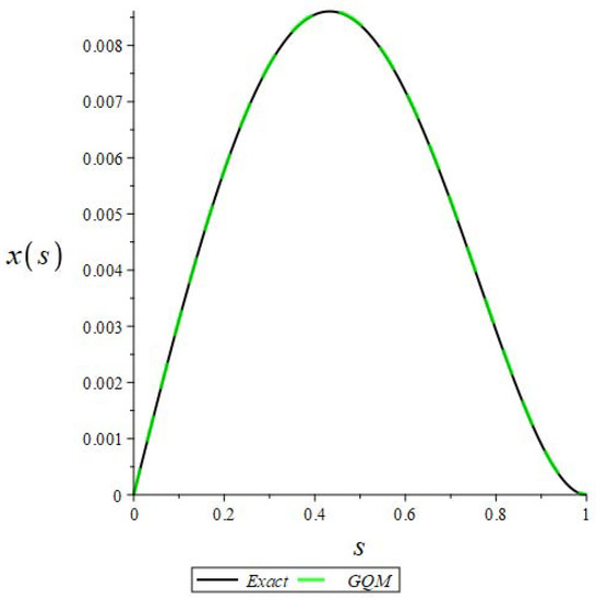
Figure 1. Comparison of the GQM with the Maple solution for $h=0.02$ (step size).

From Figure 1, we see that the curves overlap one another, which shows the efficiency and implementation of the GQM for solving (1).

Example 5 

([6]). Consider the following AVE with

$$a_{mm}=4p,a_{m,m+1}=a_{m+1,m}=p,a_{mn}=0.5,m=1,2,\cdots ,p.$$

(30)

Choose the constant vector b such that $\zeta ={\left(1,1,\cdots ,1\right)}^T$ is the actual solution of (1). We took the same initial starting vector as given in [6].

The comparison of the GQM with the MMSGP [1] and the MM [6] is given in Table 4.

Table 4. Comparison for Example 5.

		MMSGP			MM			GQM
p	K	CPU	RES	K	CPU	RES	K	CPU	RES
2	24	0.005129	5.6800× ${10}^{-7}$	2	0.029965	1.2079 × ${10}^{-12}$	1	0.005161	0
4	37	0.008701	9.7485 × ${10}^{-7}$	4	0.027864	5.5011 × ${10}^{-8}$	1	0.007681	5.0242 × ${10}^{-15}$
8	45	0.009217	5.5254 × ${10}^{-7}$	6	0.045387	6.9779 × ${10}^{-8}$	1	0.005028	3.4076 × ${10}^{-14}$
16	66	0.012458	5.8865 × ${10}^{-7}$	7	0.356930	2.0736 × ${10}^{-8}$	1	0.005253	7.2461 × ${10}^{-14}$
32	55	0.031597	8.2514 × ${10}^{-7}$	8	0.033277	4.9218 × ${10}^{-8}$	1	0.004498	2.0885 × ${10}^{-13}$
64	86	0.085621	7.6463 × ${10}^{-7}$	9	0.185753	9.0520 × ${10}^{-9}$	1	0.007191	6.6775 × ${10}^{-13}$
128	90	0.521056	6.3326 × ${10}^{-7}$	9	0.452394	1.7912 × ${10}^{-8}$	1	0.262364	3.2435 × ${10}^{-12}$

From Table 4, we observe that the GQM is more effective for solving (1). Moreover, when n increases, our proposed method is very consistent, while the other two methods require more iterations for large systems.

5. Conclusions

In this paper, we considered a two-step method for solving the AVE, and the well-known generalized Newton method was taken as the predictor step and the Gauss quadrature rule as the corrector step. The convergence was proven under certain suitable conditions. This method was shown to be effective for solving AVE (1) compared to the other similar methods. This idea can be extended to solve generalized absolute value equations. It is also interesting to study the three-point Gauss quadrature rule as the corrector step for solving the AVE.

References

- Rohn, J. A theorem of the alternatives for the equation Ax+Bx=b. Linear Multilinear Algebr. 2004, 52, 421–426. [Google Scholar] [CrossRef]
- Khan, A.; Iqbal, J.; Akgul, A.; Ali, R.; Du, Y.; Hussain, A.; Nisar, K.S.; Vijayakumar, V. A Newton-type technique for solving absolute value equations. Alex. Eng. J. 2023, 64, 291–296. [Google Scholar] [CrossRef]
- Feng, J.M.; Liu, S.Y. An improved generalized Newton method for absolute value equations. SpringerPlus 2016, 5, 1–10. [Google Scholar] [CrossRef] [PubMed]
- Feng, J.M.; Liu, S.Y. A new two-step iterative method for solving absolute value equations. J. Inequalities Appl. 2019, 2019, 39. [Google Scholar] [CrossRef]
- Shi, L.; Iqbal, J.; Arif, M.; Khan, A. A two-step Newton-type method for solving system of absolute value equations. Math. Probl. Eng. 2020, 2020, 2798080. [Google Scholar] [CrossRef]
- Noor, M.A.; Iqbal, J.; Khattri, S.; Al-Said, E. A new iterative method for solving absolute value equations. Inter. J. Phys. Sci. 2011, 6, 1793–1797. [Google Scholar]
- Noor, M.A.; Iqbal, J.; Noor, K.I.; Al-Said, E. On an iterative method for solving absolute value equations. Optim. Lett. 2012, 6, 1027–1033. [Google Scholar] [CrossRef]
- Srivastava, H.M.; Iqbal, J.; Arif, M.; Khan, A.; Gasimov, Y.M.; Chinram, R. A new application of Gauss Quadrature method for solving systems of nonlinear equations. Symmetry 2021, 13, 432. [Google Scholar] [CrossRef]
- Ali, R. Numerical solution of the absolute value equation using modified iteration methods. Comput. Math. Methods 2022, 2022, 2828457. [Google Scholar] [CrossRef]
- Ali, R.; Khan, I.; Ali, A.; Mohamed, A. Two new generalized iteration methods for solving absolute value equations using M-matrix. AIMS Math. 2022, 7, 8176–8187. [Google Scholar] [CrossRef]
- Huang, B.; Li, W. A modified SOR-like method for absolute value equations associated with second order cones. J. Comput. Appl. Math. 2022, 400, 113745. [Google Scholar] [CrossRef]
- Liang, Y.; Li, C. Modified Picard-like method for solving absolute value equations. Mathematics 2023, 11, 848. [Google Scholar] [CrossRef]
- Mangasarian, O.L.; Meyer, R.R. Absolute value equations. Lin. Alg. Appl. 2006, 419, 359–367. [Google Scholar] [CrossRef]
- Mangasarian, O.L. A generalized Newton method for absolute value equations. Optim. Lett. 2009, 3, 101–108. [Google Scholar] [CrossRef]
- Noor, M.A.; Iqbal, J.; Al-Said, E. Residual iterative method for solving absolute value equations. In Abstract and Applied Analysis; Hindawi: London, UK, 2012. [Google Scholar] [CrossRef]
- Ortega, J.M.; Rheinboldt, W.C. Iterative Solution of Nonlinear Equations in Several Variables; Academic Press: Cambridge, MA, USA, 1970. [Google Scholar]
- Yu, Z.; Li, L.; Yuan, Y. A modified multivariate spectral gradient algorithm for solving absolute value equations. Appl. Math. Lett. 2021, 21, 107461. [Google Scholar] [CrossRef]
- Zhang, Y.; Yu, D.; Yuan, Y. On the Alternative SOR-like Iteration Method for Solving Absolute Value Equations. Symmetry 2023, 15, 589. [Google Scholar] [CrossRef]
Disclaimer/Publisher’s Note: The statements, opinions and data contained in all publications are solely those of the individual author(s) and contributor(s) and not of MDPI and/or the editor(s). MDPI and/or the editor(s) disclaim responsibility for any injury to people or property resulting from any ideas, methods, instructions or products referred to in the content. |
© 2023 by the authors. Licensee MDPI, Basel, Switzerland. This article is an open access article distributed under the terms and conditions of the Creative Commons Attribution (CC BY) license (https://creativecommons.org/licenses/by/4.0/).