TE-Polarized Electromagnetic Wave Diffraction by a Circular Slotted Cylinder

Abstract

The problem of diffraction of a TE-polarized electromagnetic wave by a circular slotted cylinder is investigated. The boundary value problem in question for the Helmholtz equation is reduced to an infinite system of linear algebraic equations of the second kind (SLAE-II) using integral summation identities (ISI). A detailed study of the matrix operator of the problem is performed and its Fredholm property in the weighted Hilbert space of infinite sequences is proven. The convergence of the truncation method constructed in the paper for the numerical solution of SLAE-II is justified and the results of computations are presented and discussed, specifically considering the determination of resonance modes.

1. Introduction

As is known [1,2], for cylindrical scatterers, the physical problem of the electromagnetic wave diffraction stated initially for the system of Maxwell equations can be reduced to a boundary value problem (BVP) for the Helmholtz equation. Both numerical and analytical methods have been extensively used to solve and investigate BVPs for the system of Maxwell and Helmholtz equations in open domains.

In a variety of cases considered in the literature, BVPs for the Helmholtz equation can be reduced in one way or another to an infinite SLAE. To this end, the method of partial domains (PDM) makes it possible to find the solution of BVP in each subdomain in the form of a series with unknown coefficients using a system of orthonormalized eigenfunctions. Substitution of this expansion to the boundary and transmission conditions (some of them may be stated on fictitious boundaries separating partial domains) yields coupled (dual) summation functional equations (DAFE). The next step is to reduce DAFE to an infinite SLAE. The name of a particular version of the method depends on how this reduction is performed: direct projection [3,4], mode matching with semi-inversion [5], the method of the Riemann–Hilbert problem [6], etc.

The main idea applied in several studies for cylindrical structures employs a combination of the mode matching or the PDM methods used to reduce the considered BVP in the cross-sectional plane (with the boundary and transmission conditions stated on a set of circles and unclosed circular arcs [7,8]) to (i) an infinite SLAE initially having a trigonometric summation kernel, which is then transformed into an SLAE of the second kind (SLAE-II) with a different kernel and a canonical summation Fredholm operator acting in an appropriate Hilbert space of infinite sequences, where the reduction is performed using the so-called analytical regularization and semi-inversion as in [7,8]; or to (ii) a boundary integral equation (BIE) with integration over the strips (unclosed arcs on which the first- or the second-kind boundary conditions are stated); this BIE is then transformed into SLAE-II using different regularization and semi-inversion procedures [9,10,11]. A central point of both approaches (i), (ii) is that the SLAE-II obtained in the cited works (as a result of regularization) are considered as operator equations with canonical second-kind Fredholm operators, which makes this system useful and applicable for computations because the truncation procedure of their numerical solution can be fully justified. Many results obtained using technique (i) are reported in [10,12,13,14]. In [15], a similar method of summation identities is used to reduce the BVP for the Helmholtz equation corresponding to the scattering problem for an open resonator to a well-conditioned SLAE.

Note that in some particular cases, it is possible to obtain exact solutions by means of PDM. For example, in [16,17,18], the exact solution is constructed and the resonance modes are studied on this basis for the problem of the TE-polarized electromagnetic wave scattering on a cylindrical dielectric resonator with a circular cross section.

For the numerical solution of SLAE-II, which is a key point of its application for the problems in question, the truncation (reduction) may be used, which allows one to solve finite-dimensional systems instead of an infinite-dimensional one. The key point of the truncation method is its justification, i.e., a proof of convergence of approximate solutions obtained for the truncated (finite-dimensional) systems to the exact solution of the initial infinite-dimensional system provided that the latter exists and is unique and all function spaces are chosen correctly. In [5,19,20,21], the convergence of the truncation method in the energy space is shown, which also enforces the energy condition: the finiteness of the electromagnetic field energy in any finite spatial volume formulated as the Meixner edge condition.

Note also the recent works [22,23,24,25,26,27,28] devoted to the solution of the electromagnetic wave diffraction problems in waveguide structures with resonant regions formed by slotted rectangular resonators. In the cited works, DAFE are reduced to SLAE-II using the method of integral summation identities (ISI).

In this paper, the method of ISI is applied to solve the TE-polarized electromagnetic wave diffraction problem on a circular slotted scatterer. The setting is reduced to SLAE-II. A study of the associated infinite matrix operator is carried out and its Fredholm property is established in the appropriate weighted Hilbert space of infinite sequences. In addition, the convergence of the truncation (reduction) method used for the numerical solution of the obtained SLAE-II is proven and the results of model computations reported—in particular, the resonance modes of the structure [29,30].

A remark concerning the novelty of the developed approach should be made first: in the majority of works cited above, SLAE-II with canonical Fredholm operators are constructed as a result of complicated multi-step procedures and the final infinite SLAE-II matrices comprise the elements obtained using tedious calculations. The main feature of this study, which has served as a driving force to accomplish it, is that we have managed to construct SLAE-II directly using a much simpler one-step procedure, resulting in simple explicit representations for the SLAE entries that do not require complicated intermediate calculations.

2. Problem Statement

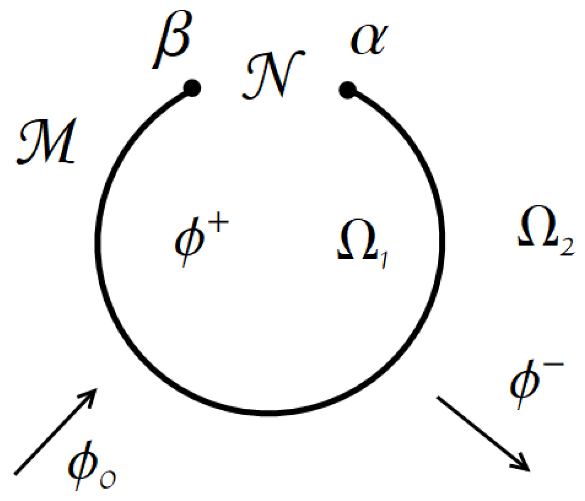
Consider the two-dimensional problem of a TE-polarized electromagnetic wave diffraction on a cylindrical resonator of circular cross-section of the radius $r=r_0$, where $(r,\theta )$ are the polar coordinates of a point in the cross-sectional plane (Figure 1). The cross-sectional region occupied by the perfectly conducting (metal) surface is denoted by $\mathcal{M}$, which is a circular arc. We assume that the resonator boundary is infinitely thin and perfectly conducting.

A mathematical model of the plane wave scattering on a perfectly conducting cylinder with a longitudinal slot is reduced to the solution of the BVP for the Helmholtz equation

$$\Delta \varphi (r,\theta )+{\kappa }^2\varphi (r,\theta )=0,$$

(1)

where ${\kappa }^2={\omega }^2\mu ϵ$ is the wave number, with respect to the function $\varphi (r,\theta )=E_3(r,\theta )$, which is the longitudinal component of the electric field vector of the total scattered field $E=\left[0,0,E_3(r,\theta )\right],$ in the entire plane except for the circular arc $\mathcal{M}$, with the boundary conditions

$${\left.\varphi \right|}_{\mathcal{M}}=0,$$

(2)

the energy finiteness condition on each compact set $Q\subset {\mathbb{R}}^2$ (Meixner’s edge condition)

$$\underset{Q}{\int }\left(\mid \varphi {\mid }^2+\mid ▽\varphi {\mid }^2\right)dv<\infty ,$$

(3)

and the Sveshnikov–Reichardt conditions at infinity, according to which the potential function $\varphi \left(\rho \right)$ can be represented as a uniformly convergent series admitting double termwise differentiation

$$\varphi \left(\rho \right)=\sum _{n=-\infty }^{\infty }{a}_n{H}_n^{\left(1\right)}\left(\kappa r\right)e^{in\theta }$$

(4)

at $r>r_0$, where $\rho =(r,\theta )$.

The total field (1)–(4) can be represented as

$$\begin{array}{c}\hfill \varphi (r,\theta )=\left\{\begin{array}{c}{\varphi }^{+}(r,\theta ),r⩽r_0,\hfill \\ {\varphi }_0(r,\theta )+{\varphi }^{-}(r,\theta ),r>r_0,\hfill \end{array}\right.\end{array}$$

(5)

where ${\varphi }_0(r,\theta )=e^{-ircos\theta }={\sum }_{n=-\infty }^{\infty }{(-i)}^n{J}_n\left(\kappa r\right)e^{in\theta }$ is the electromagnetic wave impinging on the resonator,

$$\begin{array}{cc}\hfill & {\varphi }^{+}(r,\theta )=\sum _{n=-\infty }^{+\infty }{z}_n{J}_n\left(\kappa r\right)e^{in\theta },\hfill \end{array}$$

(6)

$$\begin{array}{cc}\hfill & {\varphi }^{-}(r,\theta )=\sum _{n=-\infty }^{+\infty }{x}_n{H}_n^{\left(1\right)}\left(\kappa r\right)e^{in\theta },\hfill \end{array}$$

(7)

and for the vector $x={\left\{x_k\right\}}_{k=-\infty }^{\infty }$, the following assumption holds

$${\left\{x_k{H}_n^{\left(1\right)}\left(\kappa r\right)\right\}}_{k=-\infty }^{\infty }\in h_p=\left\{a={\left\{a_k\right\}}_{k=-\infty }^{\infty }:\sum _{k=-\infty }^{\infty }\mid a_k{\mid }^2\mid k{\mid }^p<+\infty \right\},0\le p\le 2$$

(8)

enforced due to the edge condition and the requirement that series (7) allow for differentiation so that the function ${\psi }^{-}(r,\theta )$ given by series (7) satisfies the Helmholtz equation (1) in the entire plane except for the arc of the circumference $\mathcal{M}.$

3. Reducing the Problem to SLAE-II

Consider the arc of the circle

$$\mathcal{N}=\left\{(r,\theta )|r=r_0,\alpha <\theta <\beta \right\},$$

as a “dummy” part of the boundary of the partial regions

$${\Omega }^1=\left\{(r,\theta )\mid r⩽r_0,\theta \in \left[0,2\pi \right]\right\},{\Omega }^2=\left\{(r,\theta )\mid r>r_0,\theta \in \left[0,2\pi \right]\right\}.$$

On this arc, the conjugation conditions of the first and second kind must be fulfilled

$${\left.\left[\varphi \right]\right|}_{\mathcal{N}}=0,{\left.\frac{\partial }{\partial r}\left[\varphi \right]\right|}_{\mathcal{N}}=0.$$

(9)

Let us rewrite boundary conditions (2) and (9) given representations (6) and (7).

The conditions on $\mathcal{N}:$

$$\sum _{n=-\infty }^{+\infty }{(-i)}^n{J}_n\left(\kappa r_0\right)e^{in\theta }+\sum _{n=-\infty }^{+\infty }{x}_n{H}_n^{\left(1\right)}\left(\kappa r_0\right)e^{in\theta }=\sum _{n=-\infty }^{+\infty }{z}_n{J}_n\left(\kappa r_0\right)e^{in\theta }$$

(10)

$$\sum _{n=-\infty }^{+\infty }{(-i)}^n{J}_n^{\prime }\left(\kappa r_0\right)e^{in\theta }+\sum _{n=-\infty }^{+\infty }{x}_n{H}_n^{{\left(1\right)}^{\prime }}\left(\kappa r_0\right)e^{in\theta }=\sum _{n=-\infty }^{+\infty }{z}_n{J}_n^{\prime }\left(\kappa r_0\right)e^{in\theta };$$

(11)

the conditions on $\mathcal{M}:$

$$\sum _{n=-\infty }^{+\infty }{(-i)}^n{J}_n\left(\kappa r_0\right)e^{in\theta }+\sum _{n=-\infty }^{+\infty }{x}_n{H}_n^{\left(1\right)}\left(\kappa r_0\right)e^{in\theta }=0,$$

(12)

$$\sum _{n=-\infty }^{+\infty }{z}_n{J}_n\left(\kappa r_0\right)e^{in\theta }=0.$$

(13)

The following statement is valid concerning the equivalent reduction of the initial BVP to an infinite SLAE of the second kind (SLAE-II).

Theorem 1. 

The boundary value problem (1)–(4) of the $TE$-polarized electromagnetic wave diffraction on a circular slot resonator is equivalent to an infinite system of linear algebraic equations of type II (SLAE-II)

$$\left(I+A\right)\tilde{x}=y,$$

(14)

where

$$A=\Vert -{\tilde{\gamma }}_j{K}_{kj}{\Vert }_{k,j=-\infty }^{\infty },K_{k,j}=\sum _{m=-\infty }^{+\infty }\frac{1}{{\tilde{\gamma }}_m}{M}_{mk}{N}_{jm},{\tilde{\gamma }}_m=\left(\frac{J_m^{\prime }\left(\kappa \right)}{J_m\left(\kappa \right)}-\frac{H_m^{{\left(1\right)}^{\prime }}\left(\kappa \right)}{H_m^{\left(1\right)}\left(\kappa \right)}\right),$$

(15)

$$y={\left\{\sum _{m=-\infty }^{\infty }{(-i)}^m{J}_m\left(\kappa r_0\right)M_{mk}\right\}}_{k=-\infty }^{\infty },$$

(16)

$$N_{nm}=\frac{1}{2\pi }\underset{\mathcal{N}}{\int }{e}^{i\alpha (n-m)}d\alpha ,M_{mk}=\frac{1}{2\pi }\underset{\mathcal{M}}{\int }{e}^{i\alpha (m-k)}d\alpha ={\delta }_{mk}-N_{mk},$$

(17)

with respect to the unknown vector of coefficients $\tilde{x}={\left\{{\tilde{x}}_k\right\}}_{k=-\infty }^{\infty }\in h_p,0\le p\le 2$.

For the vectors $x={\left\{x_k\right\}}_{k=-\infty }^{\infty }$ and $z={\left\{z_k\right\}}_{k=-\infty }^{\infty }$, the following relations hold:

$$z_k={\tilde{x}}_k{\left(J_k\left(\kappa r_0\right)\right)}^{-1}+{(-i)}^k,x_k={\tilde{x}}_k{\left(H_k^{\left(1\right)}\left(\kappa r_0\right)\right)}^{-1}k=0,\pm 1,\pm 2,\dots$$

(18)

First, using the method of ISI, we reduce the intial BVP (1)–(4) to SLAE (14) and then prove the Fredholm property of the matrix operator corresponding to (14), which in its turn means that SLAE (14) in its structure is indeed an SLAE-II, i.e., a canonical Fredholm operator equation.

It follows from (10), (12) and (13) that (10) holds on both $\mathcal{M}$ and $\mathcal{N}$. Note that in the course of the solution, we can express vector z in terms of x by Formula (18). Substitute this expression into (11) and (13) and exclude $z_n$:

$$\sum _{n=-\infty }^{+\infty }{x}_n{H}_n^{\left(1\right)}\left(\kappa r_0\right)e^{in\theta }{\tilde{\gamma }}_n=0,\theta \in \mathcal{N},$$

(19)

$$\sum _{n=-\infty }^{+\infty }{x}_n{H}_n^{\left(1\right)}\left(\kappa r_0\right)e^{in\theta }=\sum _{n=-\infty }^{+\infty }{(-i)}^n{J}_n\left(\kappa r_0\right)e^{in\theta },\theta \in \mathcal{M},$$

(20)

where ${\displaystyle {\tilde{\gamma }}_n=\left(\frac{J_n^{\prime }\left(\kappa r_0\right)}{J_n\left(\kappa r_0\right)}-\frac{H_n^{{\left(1\right)}^{\prime }}\left(\kappa r_0\right)}{H_n^{\left(1\right)}\left(\kappa r_0\right)}\right)}$.

Introduce the summation kernel

$$K(\theta ,\delta )=\sum _{m=-\infty }^{+\infty }\frac{1}{{\tilde{\gamma }}_n}{e}^{im\theta }{e}^{-im\delta }.$$

The following equation holds:

$$\underset{\mathcal{M}\cup \mathcal{N}}{\int }\left(\sum _{n=-\infty }^{+\infty }{x}_n{\tilde{\gamma }}_n{H}_n^{\left(1\right)}\left(\kappa r_0\right)e^{in\delta }\right)K(\theta ,\delta )d\delta =\sum _{n=-\infty }^{+\infty }{x}_n{H}_n^{\left(1\right)}\left(\kappa r_0\right)e^{in\theta }$$

called the integral summation identity (ISI).

From ISI and (19), we obtain

$$\sum _{n=-\infty }^{+\infty }{x}_n{H}_n^{\left(1\right)}\left(\kappa r_0\right)e^{in\theta }=\sum _{n=-\infty }^{+\infty }{x}_n{\tilde{\gamma }}_n{H}_n^{\left(1\right)}\left(\kappa r_0\right)\sum _{m=-\infty }^{+\infty }\frac{1}{{\tilde{\gamma }}_m}{M}_{nm}{e}^{im\theta }$$

(21)

Construct a projection of (20) and (21) onto the function system $e^{-ik\theta }$, which yields

$$x_k{H}_k^{\left(1\right)}\left(\kappa r_0\right)-\sum _{j=-\infty }^{\infty }{x}_j{H}_j^{\left(1\right)}\left(\kappa r_0\right){\tilde{\gamma }}_j{K}_{kj}=\sum _{m=-\infty }^{\infty }{(-i)}^m{J}_m\left(\kappa r_0\right)M_{mk},k=\pm 1,\pm 2,\dots$$

(22)

In system (22), perform the substitution of variables

$${\tilde{x}}_k=x_k{H}_k^{\left(1\right)}\left(\kappa r_0\right),k=0,\pm 1,\pm 2,\dots$$

(23)

and obtain finally SLAE (14) with respect to the vector $\tilde{x}={\left\{{\tilde{x}}_k\right\}}_{k=-\infty }^{\infty }.$

Let us now proceed to the proof of the Fredholm property of the SLAE matrix operator. The following statement holds.

Theorem 2. 

Matrix operator $I+A$ corresponding to SLAE (14) is a (canonical) Fredholm operator in the Hilbert space $h_p$.

An equivalent formulation: SLAE (14) is an SLAE-II in the space $h_p$.

Explain the equivalence of the above formulations. As is known, for an SLAE of the form (14) to be an SLAE-II in $h_p$, operator A must be compact in $h_p$; then, $I+A$ by Nikolski’s criterion [31,32] will be a (canonical) Fredholm operator in $h_p$.

Thus, it is sufficient to prove the following.

Theorem 3. 

The operator $A:h_p\to h_p$ defined by (14) is compact in $h_p$.

To prove this theorem, let us use the sufficient condition of the compactness of a matrix operator in a Hilbert space [5,21,33].

Lemma 1. 

Let a matrix operator A defined by its infinite matrix (15) be given. Then, if the condition

$$\sum _{k,j=-\infty }^{\infty }\mid a_{k,j}{\mid }^2\mid k{\mid }^p<\infty ,0\le p\le 2$$

(24)

holds, then A is compact in $h_p$.

Before proceeding to the necessary proof of convergence of dual series (24), let us examine the asymptotic properties of the entries of matrix A.

To this end, consider in more detail the expression for ${\tilde{\gamma }}_m$:

$$\begin{array}{c}{\tilde{\gamma }}_m=\frac{J_m^{\prime }\left(\kappa \right)}{J_m\left(\kappa \right)}-\frac{H_m^{{\left(1\right)}^{\prime }}\left(\kappa \right)}{H_m^{\left(1\right)}\left(\kappa \right)}=\frac{\frac{m}{\kappa }{J}_m\left(\kappa \right)-J_{m+1}\left(\kappa \right)}{J_m\left(\kappa \right)}-\\ -\frac{\frac{m}{\kappa }{H}_m^{\left(1\right)}\left(\kappa \right)-H_{m+1}^{\left(1\right)}\left(\kappa \right)}{H_m^{\left(1\right)}\left(\kappa \right)}=\frac{H_{m+1}^{\left(1\right)}\left(\kappa \right)}{H_m^{\left(1\right)}\left(\kappa \right)}-\frac{J_{m+1}\left(\kappa \right)}{J_m\left(\kappa \right)}.\end{array}$$

(25)

For the Bessel functions, there are asymptotic relations [34]

$$J_m\left(\kappa \right)\sim \frac{1}{\Gamma (m+1)}{\left(\frac{\kappa }{2}\right)}^m,\left|H_m^{\left(1\right)}\left(\kappa \right)\right|\sim \Gamma \left(m\right){\left(\frac{2}{\kappa }\right)}^m,m\to \infty ,$$

(26)

where $\Gamma \left(m\right)$ is the Euler Gamma function, from which it follows that

$$\frac{J_{m+1}\left(\kappa \right)}{J_m\left(\kappa \right)}\sim \frac{1}{m},\left|\frac{H_{m+1}^{\left(1\right)}\left(\kappa \right)}{H_m^{\left(1\right)}\left(\kappa \right)}\right|\sim \frac{\Gamma (m+1)}{\Gamma \left(m\right)}=m,m\to \infty .$$

(27)

Thus, given (27), we obtain the asymptotic relation

$$\left|{\tilde{\gamma }}_m\right|\sim m,m\to \infty .$$

(28)

For numbers $N_{n,m}$ defined by (17), we have the explicit formulas

$$N_{n,m}=\left\{\begin{array}{c}{\displaystyle \frac{i\left(e^{-i(m-n)\beta }-e^{-i(m-n)\alpha }\right)}{2(m-n)\pi },n\ne m,}\hfill \\ {\displaystyle \frac{\beta -\alpha }{2\pi },n=m,}\hfill \end{array}\right.$$

which, in the particular case $\beta =\pi ,\alpha =0$, can be written in a simpler form:

$$N_{n,m}=\left\{\begin{array}{c}{\displaystyle \frac{i\left({(-1)}^{n-m}-1\right)}{2(m-n)\pi },n\ne m,}\hfill \\ {\displaystyle \frac{1}{2},n=m.}\hfill \end{array}\right.$$

(29)

Obviously, there is an estimate

$$\left|N_{n,m}\right|<\left\{\begin{array}{c}{\displaystyle \frac{1}{|m-n|},n\ne m,}\hfill \\ {\displaystyle 1,n=m,}\hfill \end{array}\right.$$

which we will use in what follows.

Now, we can construct an estimation for the summation kernel $K_{kj}$ using the triangle inequality

$$\mid K_{k,j}\mid \le \left|\frac{1}{k}{M}_{k,k}{N}_{j,k}\right|+\left|\frac{1}{j}{M}_{j,k}{N}_{j,j}\right|+R,$$

(30)

where

$$R=\sum _{m=-\infty ,m\ne k,j}^{+\infty }{\left|m^3(\frac{k}{m}-1)(1-\frac{j}{m})\right|}^{-1},$$

is a rapidly converging series (as sum of inverse cubes) and $R\to 0$ at $k,j\to \infty$. Thus, we have

$$\left|K_{kj}\right|<\left\{\begin{array}{c}{\displaystyle \left|\frac{k+j}{kj(k-j)}\right|,k\ne j,}\hfill \\ {\displaystyle \frac{1}{k},k=j.}\hfill \end{array}\right.$$

(31)

From the above estimates follow asymptotic relations for the entries of matrix A

$$\left|a_{k,j}\right|=O(\mid kj{\mid }^{-1}),\mid k\mid ,\mid j\mid \to \infty .$$

(32)

Using the above asymptotics and estimates, we can use Dalembert’s sufficient condition [35] to prove the dual series (24) convergence.

Lemma 2. 

If, for the dual series ${\sum }_{k,j}{u}_{kj}$, the conditions

$$\underset{k\to \infty }{lim}\left|\frac{u_{k+1,j}}{u_{k,j}}\right|<1,$$

(33)

hold for all j and

$$\underset{j\to \infty }{lim}\left|\frac{u_{k,j+1}}{u_{k,j}}\right|<1,$$

(34)

for all k, then the dual series converges.

Let us prove the fulfillment of these relations for series (24). From (31), (33) and (34), we have

$$\begin{array}{c}\left|\frac{u_{k+1,j}}{u_{k,j}}\right|={\left|\frac{\frac{1}{{\tilde{\gamma }}_j}{K}_{k+1,j}}{\frac{1}{{\tilde{\gamma }}_j}{K}_{k,j}}\right|}^2{\left(\frac{k+1}{k}\right)}^p={\left|\frac{K_{k+1,j}}{K_{k,j}}\right|}^2{\left(\frac{k+1}{k}\right)}^p,\end{array}$$

(35)

$$\begin{array}{c}\left|\frac{u_{k,j+1}}{u_{k,j}}\right|={\left|\frac{\frac{1}{{\tilde{\gamma }}_{j+1}}{K}_{k,j+1}}{\frac{1}{{\tilde{\gamma }}_j}{K}_{k,j}}\right|}^2.\end{array}$$

(36)

Taking into account the estimate for kernel $K_{kj}$, recast the last relations in the form

$$\begin{array}{c}\left|\frac{u_{k+1,j}}{u_{k,j}}\right|={\left|\frac{k(k+j+1)(k-j)}{(k+1)(k+1-j)(k+j)}\right|}^2{\left(\frac{k+1}{k}\right)}^p,\end{array}$$

(37)

$$\begin{array}{c}\left|\frac{u_{k,j+1}}{u_{k,j}}\right|={\left|\frac{(k-j)(k+j+1)}{(k+j)(k-j-1)}\right|}^2.\end{array}$$

(38)

Note that inequality (38) does not contain p and holds for any k and j, such that $k\ne j+1$.

Consider (37) in more detail and rewrite it as

$$\left|\frac{u_{k+1,j}}{u_{k,j}}\right|={\left|\frac{(k+j+1)(k-j)}{(k+1-j)(k+j)}\right|}^2{\left(\frac{k+1}{k}\right)}^p{\left(\frac{k}{k+1}\right)}^2<1.$$

(39)

The last inequality holds for $0\le p\le 2$.

Now, let us complete the proof of the equivalence.

Suppose that BVP (1)–(4) has the unique classical solution. Then, the solution expansion coefficients in (5)–(7) satisfy SLAE-II (14) as elements of space $h_p(0\le p<2)$, which follows from Theorem 1.

Next, assume that function $\varphi$ is defined by series (5)–(7) with the expansion coefficients that solve SLAE-II (14). Let us check the fulfillment of the edge condition (3). Suppose that

$$Q=Q^1\bigcup Q^2,Q^1\subset {\Omega }^1,Q^2\subset {\Omega }^2;$$

(40)

then, the energy integral over compact set Q can be represented as

$$\begin{array}{c}\underset{Q}{\int }\left(\mid \varphi {\mid }^2+\mid ▽\varphi {\mid }^2\right)dv=\underset{Q^1}{\int }\left(\mid {\varphi }^{+}{\mid }^2+\mid ▽{\varphi }^{+}{\mid }^2\right)dv+\hfill \\ \hfill +\underset{Q^2}{\int }\left(\mid {\varphi }_0+{\varphi }^{-}{\mid }^2+\mid ▽\left({\varphi }_0+{\varphi }^{-}\right){\mid }^2\right)dv,\end{array}$$

(41)

The convergence of the integral over the domain $Q^1$ is obvious; therefore, of particular interest is the integral

$$\underset{Q^2}{\int }{\left|▽\left({\varphi }_0+{\varphi }^{-}\right)\right|}^{2}dv.$$

(42)

Considering the convergence of (42), we have

$$\begin{array}{c}{\left|▽\left({\varphi }_0+{\varphi }^{-}\right)\right|}^2={\left(\sum _{n=-\infty }^{\infty }n{e}^{in\theta }\left({(-i)}^n{J}_n\left(\kappa r\right)+x_n{H}_n^{\left(1\right)}\left(\kappa r\right)\right)\right)}^2+\hfill \\ \hfill +{\left(\sum _{n=-\infty }^{\infty }{e}^{in\theta }\kappa \left({(-i)}^n{J}_n^{{}^{\prime }}\left(\kappa r\right)+x_n{H}_n^{{\left(1\right)}^{\prime }}\left(\kappa r\right)\right)\right)}^2.\end{array}$$

(43)

Taking into account (26), write down the asymptotics for the series term

$$\left|n{e}^{in\theta }\left({(-i)}^n{J}_n\left(\kappa r\right)+x_n{H}_n^{\left(1\right)}\left(\kappa r\right)\right)\right|\sim \left|n{\tilde{x}}_n\right|,\left|n\right|\to \infty$$

(44)

where ${\tilde{x}}_n=x_n{H}_n^{\left(1\right)}\left(\kappa r\right).$

Thus, the integral over $Q^2$ converges in view of (43) and (8) for $p=2$.

We see that $\varphi$ satisfies the Helmholtz equation (termwise) in the entire plane except for the arc $\mathcal{M}$, boundary conditions (2) that follow from the construction of the SLAE, the edge conditions (3) and the conditions at infinity due to the explicit representation of the solution as (7) in the external (unbounded) domain.

This completes the proof of the equivalence and Theorem 1.

4. Convergence of the Truncation Method

Let X and $\overline{X}$ be, respectively, the linear spaces of infinite-dimensional vectors $x=(x_1,x_2,\dots )$ and n-dimensional vectors $\overline{x}=(x_1,x_2,\dots ,x_n)$. From the definition, we can say that the space $\overline{X}$ is an approximation of X and is obtained by truncating the vectors starting from the $n+1$st component.

Consider operators S and T acting according to

$$\begin{array}{cc}\hfill & S:{\overline{x}}^n\to x=(x_1,x_2,\dots ,x_n,0,0,\dots ),\hfill \end{array}$$

(45)

$$\begin{array}{cc}\hfill & T:x\to {\overline{x}}^n=(x_1,x_2,\dots ,x_n).\hfill \end{array}$$

(46)

We will call S and T the interpolation and approximation operators, respectively. Hereafter, we will assume that $X=h_p,\overline{X}={\mathbb{C}}^n.$

Write the approximating equation for (14) as

$$\overline{F}{\overline{x}}^n={\overline{y}}^n,$$

(47)

where $\overline{F}=\overline{I}+\overline{A}$ and n is the truncation parameter (reduction), which determines the dimensionality of the system. If the approximation is sufficiently accurate (the truncation parameter n is large enough), one should expect that the solution vectors x and $\overline{x}$ of the exact (11) and approximating (13) equations, respectively, should be close with respect to the norm of the corresponding spaces.

As part of the complete justification of the truncation method for an SLAE using an approximation scheme, the following questions must be answered:

• Uniqueness of the solution to the exact equation;
• Uniqueness of the solution to the approximating equations;
• Error estimation of the approximate solution;
• Completeness of space X.

Note that the first condition is ensured by the Fredholm property of the operator $F=I+A$; the third condition ensures that the limit of the sequence of approximate solutions belongs to space X.

The following theorem is valid concerning the S-convergence of the approximate solution of approximating Equation (47) to the solution of exact Equation (14).

Theorem 4. 

Let $x\in D\left(F\right),$ where $D\left(F\right)$ is the operator domain, $\overline{x}\in D\left(\overline{F}\right)$, with ${\overline{S}}_X\overline{x}\in D\left(F\right)$ for any n. Then, if

1. 

operator F has a bounded left inverse;

2. 

starting from a certain number (at least), the solutions $\overline{x}$ of the approximating equations are unique;

3. 

the sequence $\overline{y}$ S-converges to y;

4. 

sequence $\overline{F}$ strongly $TS$-converges to F;

5. 

sequence $ST$-converges uniformly to I;

6. 

operators S are uniformly bounded.

Then, the sequence $\overline{x}$ S-converges to x.

The second condition can be verified using the following statement.

Lemma 3. 

Let $S\overline{x}\in D\left(F\right)$ for any $\overline{x}\in D\left(\overline{F}\right)$ and operators S and T are bounded. Assume that operator F has a bounded left inverse and the following conditions hold:

$$\begin{array}{c}\parallel \left(\overline{F}-TFS\right)\overline{x}\parallel \le m_1\left(n\right)\parallel \overline{x}\parallel ,\end{array}$$

(48)

$$\begin{array}{c}\parallel \left(ST-I\right)FS\overline{x}\parallel \le m_2\left(n\right)\parallel \overline{x}\parallel ,\end{array}$$

(49)

where $m_1$ and $m_2$ are some constants independent of $\overline{x}$. Then, if

$$\left(m_1\left(n\right)\parallel S\left|\right|+m_2\left(n\right)\right)\parallel T\parallel <\infty ,$$

(50)

then operator $\overline{F}$ has a bounded inverse.

Detailed proof of these statements is given in [36,37]. Therefore, in this paper, we only check the fulfillment of the condition (50).

The following theorem holds stating the convergence of approximate solutions to the exact solution.

Theorem 5. 

The sequence of solutions of approximating Equation (47) S-converges to the solution of SLAE-II (14).

In the case $X=h_p$, it can be shown that

$$m_1=m_1\left(n\right)=0,\parallel S\parallel |=\parallel T\parallel =1.$$

Thus, it follows from (50) that if

$$m_2^2\left(n\right)\le ∥|F∥{|}_{h_p}\le \sum _{k,j=-\infty }^{\infty }{\left|f_{k,j}\right|}^2{\left|k\right|}^p<\infty ,$$

(51)

then operator F is compact and the sequence of approximate solutions S-converges to the exact solution.

5. Resonance Frequencies

Initial BVP (1)–(5) with ${\varphi }_0(r,\theta )=0$ can be considered as a boundary eigenvalue problem (BEP) with respect to spectral parameter $\kappa$ or $\omega$. The use of the Sveshnikov–Reichardt conditions at infinity in the BEP statement enables one to take into account and determine any complex eigenvalues.

In the absence of the slot, BVP (1)–(5) splits into two problems, internal in a disk of radius $r_0$ and external in the domain outside the disk with boundary condition (2) stated on the whole circle $r=r_0$. The former has real eigenvalues ${\kappa }_{nm}={\mu }_{nm}$ forming a set of isolated real points $\mathcal{K}={\cup }_{n,m}{\kappa }_{nm}$ on the complex plane $\kappa$; here, ${\mu }_{nm}$ are zeros of the Bessel functions $J_n\left(z\right)$, $n=0,1,\dots$, $m=1,2,\dots$ Using the technique of operator-valued functions (OVFs) [38] developed in [39,40,41], reducing BEP to a boundary integral equation (BIE) with integration over the fictitious boundary, a circular arc replacing the slot $\mathcal{N}$, and separating the principal parts (in the form of meromorphic operator pencils) of the obtained finite-meromorphic boundary integral OVFs with respect to both the spatial variables and spectral parameter, one can show that, at least for a sufficiently narrow slot, BEP (1)–(5) has isolated complex eigenvalues with the negative imaginary parts situated in small proximities of ${\kappa }_{nm}={\mu }_{nm}$. Finally, one can verify that the eigenvalue spectrum $\mathcal{K}\left(\mathcal{N}\right)={\cup }_{n,m}{\kappa }_{nm}\left(\mathcal{N}\right)$ of BEP (1)–(5) can be considered as a regular perturbation of the ’non-perturbed’ real spectrum $\mathcal{K}$ of the internal BEP in the partial domain, the disk $r=r_0$, with respect to the diameter of the slot. In addition, the points of $\mathcal{K}\left(\mathcal{N}\right)$ merge with the points of $\mathcal{K}$ as the diameter diam$\mathcal{N}$ of the slot (distance d between the slot edges) tends to zero, ${\kappa }_{nm}\left(\mathcal{N}\right)={\kappa }_{nm}\left(d\right)\to {\kappa }_{nm}$, $d\to 0$. From the physical viewpoint, this part $\mathcal{K}\left(\mathcal{N}\right)$ of the spectrum is the most important because the corresponding resonance frequencies (RFs), ${\kappa }_{nm}\left(\mathcal{N}\right)\approx {\mu }_{nm}-i{\alpha }_{nm}$, $i^2=-1$, ${\alpha }_{nm}>0$, have a high Q-factor, i.e., small imaginary parts. RFs with the smallest indices $n=0,1$, $m=1,2,$ have the largest Q-factor. Taking d as a small parameter, one can estimate ${\alpha }_{nm}<Cd$, $C=$const, applying the technique [42] to BIE with an integral operator having a logarithmic singularity of the kernel.

Below, the results of the RF calculations are reported that reveal among all the occurrence of the ’perturbed’ high-Q RFs ${\kappa }_{nm}\left(\mathcal{N}\right)={\kappa }_{nm}\left(d\right)\to {\kappa }_{nm}$ in small vicinities of ’non-perturbed’ RFs ${\kappa }_{nm}={\mu }_{nm}$ of the shielded cylindrical resonator of a circular cross section.

6. Results of Model Computations

For the approximate solution of SLAE-II (14), we will use the method of truncation (reduction) described and justified in the previous section.

To this end, write the truncated system corresponding to (14) in the form

$$F_N{x}^N=y^N,$$

(52)

where N is the truncation parameter.

In what follows, we will perform all calculations for the truncation parameter $N=20$, and resonator parameters $r_0=1,$$\mathcal{N}=\left[0,\pi /30\right]$ measured in dimensionless units. In this case, we will obtain a system of dimension $41\times 41$.

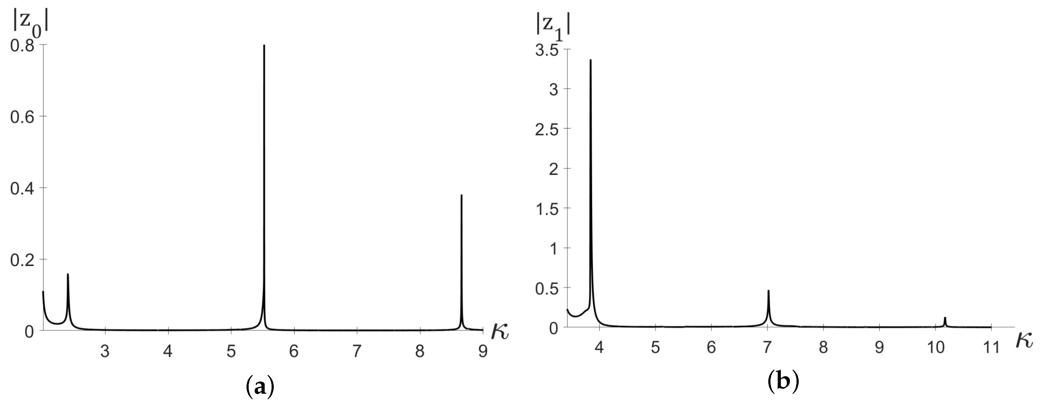
Figure 2 shows the resonance curves: the absolute values of coefficients $z_0$ and $z_1$ of the solution series expansion (6) plotted against spectral parameter $\kappa$. It can be seen that the moduli of the coefficients increase sharply in the neighborhood of the zeros ${\mu }_{nm}$ of the Bessel functions $J_n\left(z\right)$, as it follows from the occurrence of RFs ${\kappa }_{nm}\left(\mathcal{N}\right)\approx {\mu }_{nm}-i{\alpha }_{nm}$, ${\alpha }_{nm}>0$, close to these points for narrow slots; sharp peaks correspond to the real values $\kappa \approx {\mu }_{nm}$.

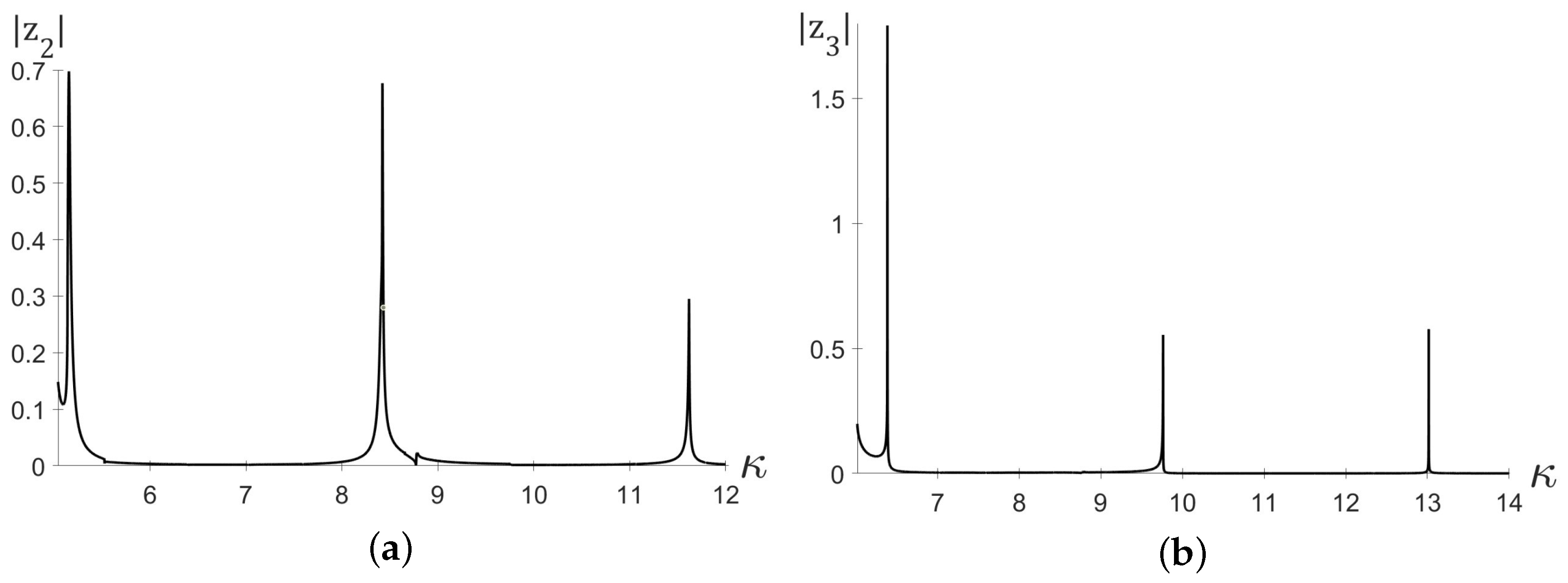
Similar resonance curves are shown in Figure 3 for coefficients $z_2$ and $z_3$.

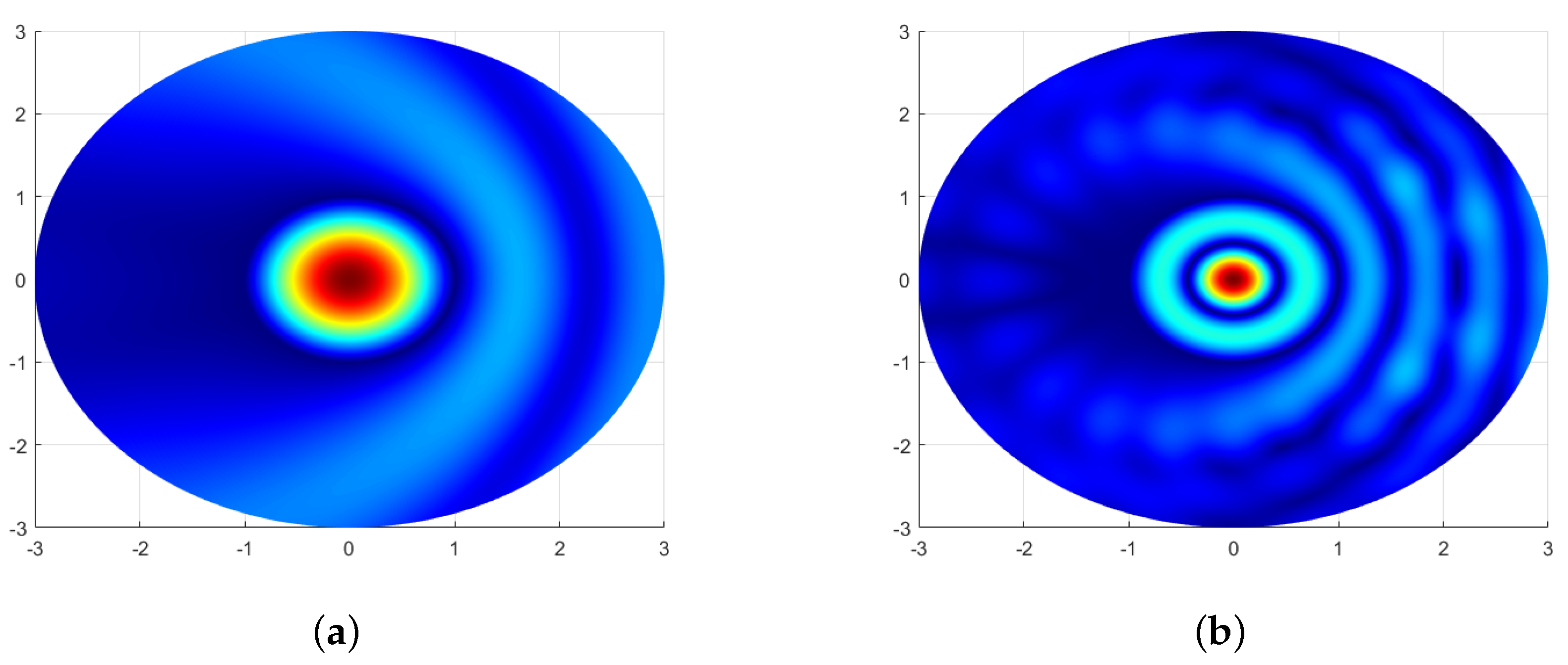
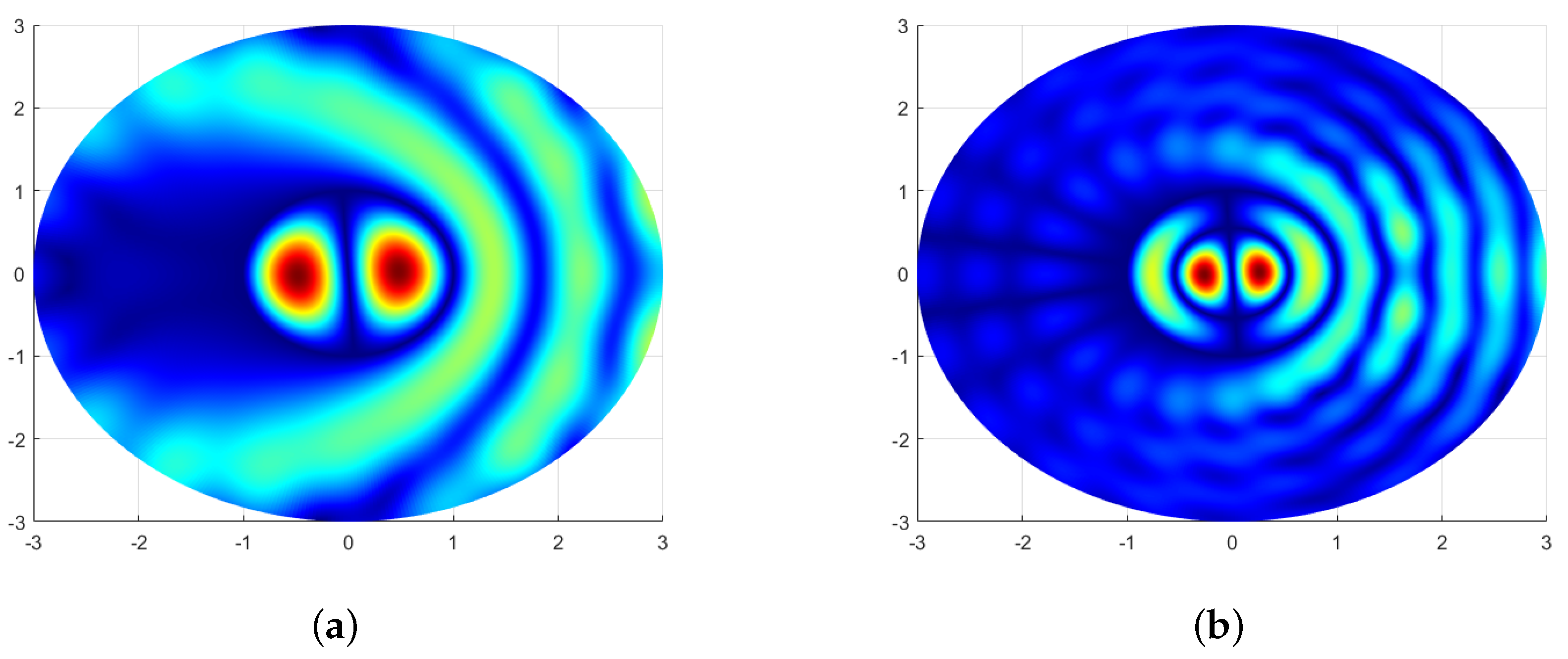
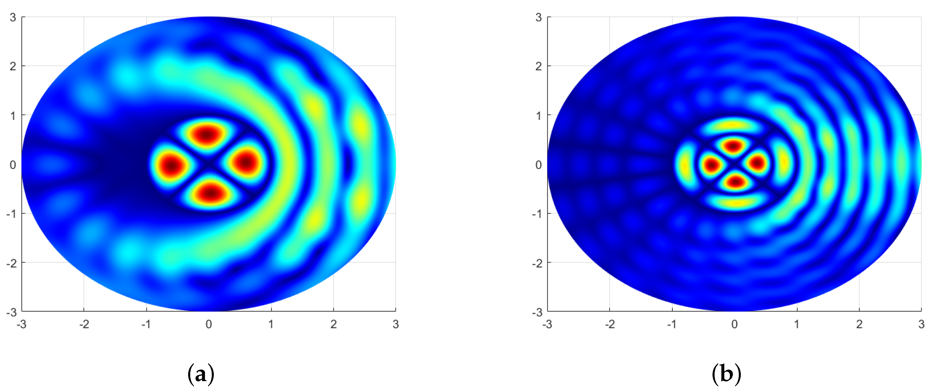
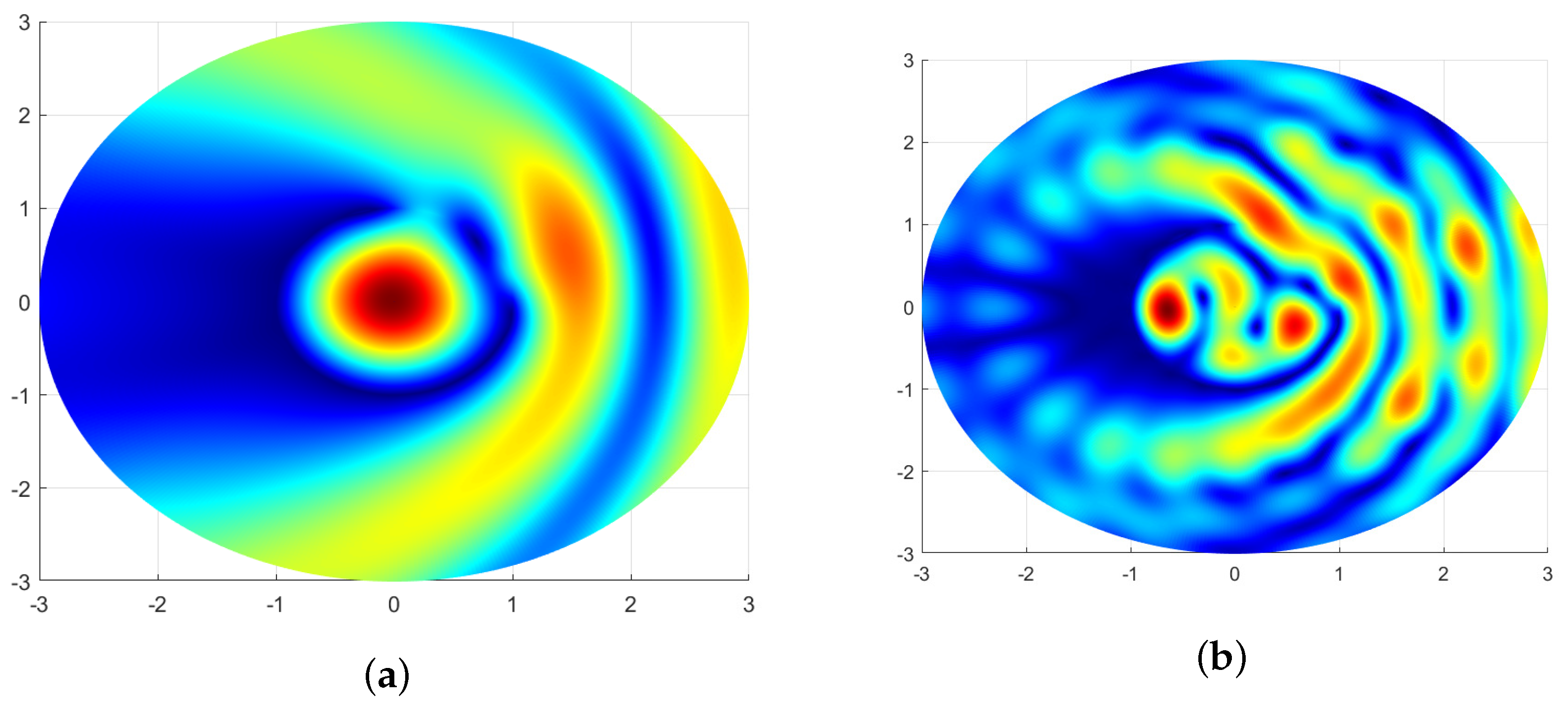
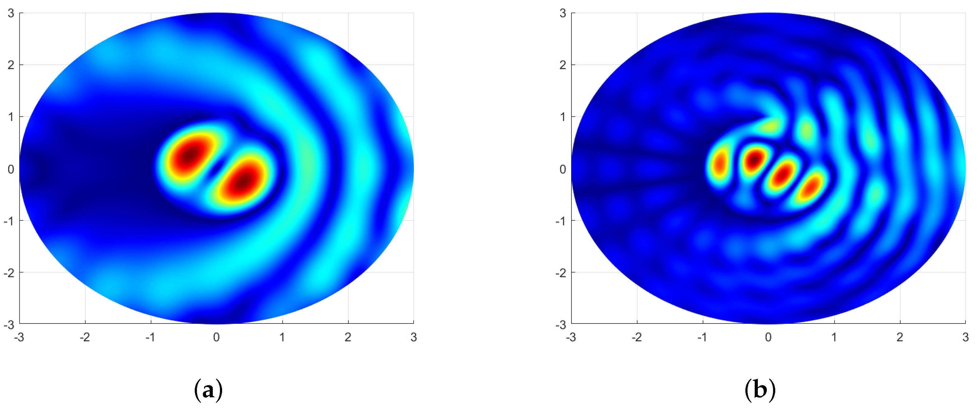
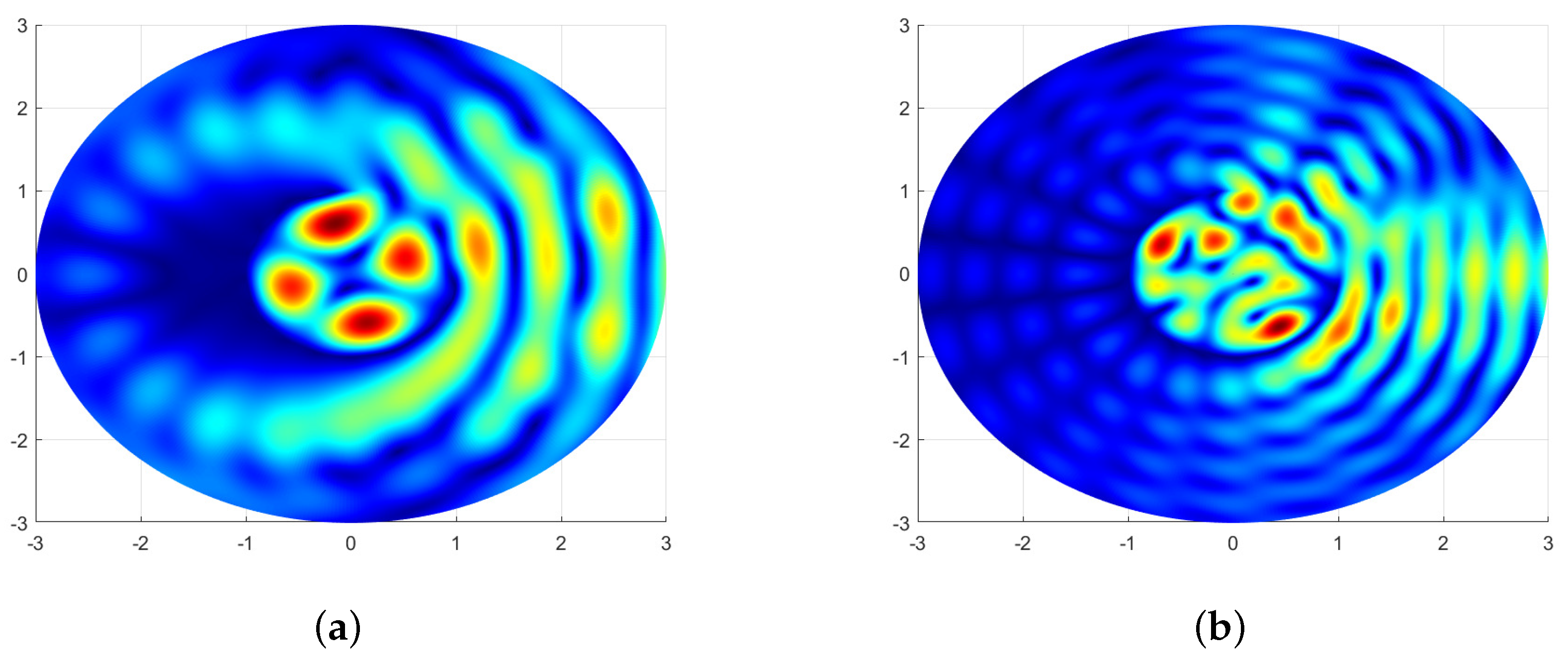
Figure 4, Figure 5 and Figure 6 show the graphs of the amplitude of the electromagnetic field component $E_z$ in the cross-section of the circular slotted scatterer for the $\mathcal{N}=[0,\pi /30]$ and lowest modes: $E_{01},E_{02},E_{11},E_{12},E_{21},E_{22}.$ Similar graphs are shown in Figure 7, Figure 8 and Figure 9 at $\mathcal{N}=[0,\pi /2]$.

One can see that the amplitude field patterns of the circular slotted scatterer with a narrow slot perfectly match the field patterns of the resonance fields in the ’non-perturbed’ circular resonator without a slot governed by the index n of the corresponding eigenfunction, the Bessel functions $J_n\left(z\right)$, $n=0,1,2$, of the internal partial domain, and the disk of the radius $r=r_0$.

7. Conclusions

In this paper, the two-dimensional TE-polarized electromagnetic wave diffraction problem on a slotted resonator has been investigated in detail. The BVP for the Helmholtz equation corresponding to the physical diffraction problem has been reduced equivalently to an SLAE-II by the method of ISI.

It has been shown that the infinite matrix operator associated with SLAE-II is a canonical Fredholm operator in the weighted Hilbert space of infinite sequences chosen in accordance with the edge condition.

With the help of an abstract projection scheme, the convergence of the approximate truncation (reduction) method used for the approximate solution of SLAE-II has been proven.

On the basis of the performed model computations, the RF approximate values have been determined. The resonance curves and the TE-polarized electromagnetic field potential function amplitude diagrams close to RFs have been constructed. It has been shown that the calculated RFs are regular pertubations of the frequency spectrum of the circular resonator without a slot.

The performed study is the first and most necessary step towards the analysis of more complicated open cylindrical resonators. Other resonator families that can be now directly investigated using the developed technique of infinite SLAE-II are, above all, one or several partially shielded dielectric rods of circular and arbitrary cross-sections.