Scaled Muth–ARMA Process Applied to Finance Market
Abstract
1. Introduction
- Conditional, by the regression approach or data-based. First, Benjamim et al. [8] proposed the generalized ARMA process (GARMA) with a marginal distribution from the exponential family (from the discrete point of view: Poisson, binomial, …; from the continuous point of view Gaussian, gamma, inverse Gaussian, …). Rocha and Cribari-Neto [9] introduced the beta ARMA (BARMA) model for the analysis of proportions. The Kumaraswamy ARMA (KARMA) model, introduced by Bayer et al. [10], has been used for hydrological data. Recently, Almeida and Nascimento [4] introduced the -ARMA process to describe intensities in synthetic aperture radar images.
- Non-conditional or innovations-based:
- –
- –
2. The sMuth–ARMA Process: Estimation and Forecasting
- is the error term having a recursive nature, although it can be defined with a martingale difference nature, such as the approach adopted by Zheng et al. [22] associated to Equation (6). As discussed by Scher et al. [23] (p. 3), we adopt the error term in Equation (6), which is in a residual fashion; i.e., a stochastic process, such as innovations in standard ARMA models, is not represented. The time series outcomes designed from our model come from a conditional distribution, and the respective moving average error, , represents the difference between an observed quantity, , and the corresponding model-based quantity, .
- denotes the intercept.
- is a set of k other time series that occur together with the worked series, . Although we did not focus on an exogenous variable in this paper, we opted to explicitly refer to it in Equation (6) by generality.
- is a vector of unknown parameters associated with the covariates ; and
- and are the parameter vectors of the AR and MA structures, respectively.
2.1. Generator of the sMuth–ARMA Model
- sM-AR(1): , or, equivalently, ;
- sM-MA(1): or, equivalently, ;
- sM-ARMA(1,1): or, equivalently,
- 1:
- Define values for the parameters , , , and for pairs such that and ;
- 2:
- Calculate (for ) using:
- 3:
- Generate for .
- 4:
- Repeat steps 2 and 3 until n values of the series are generated.
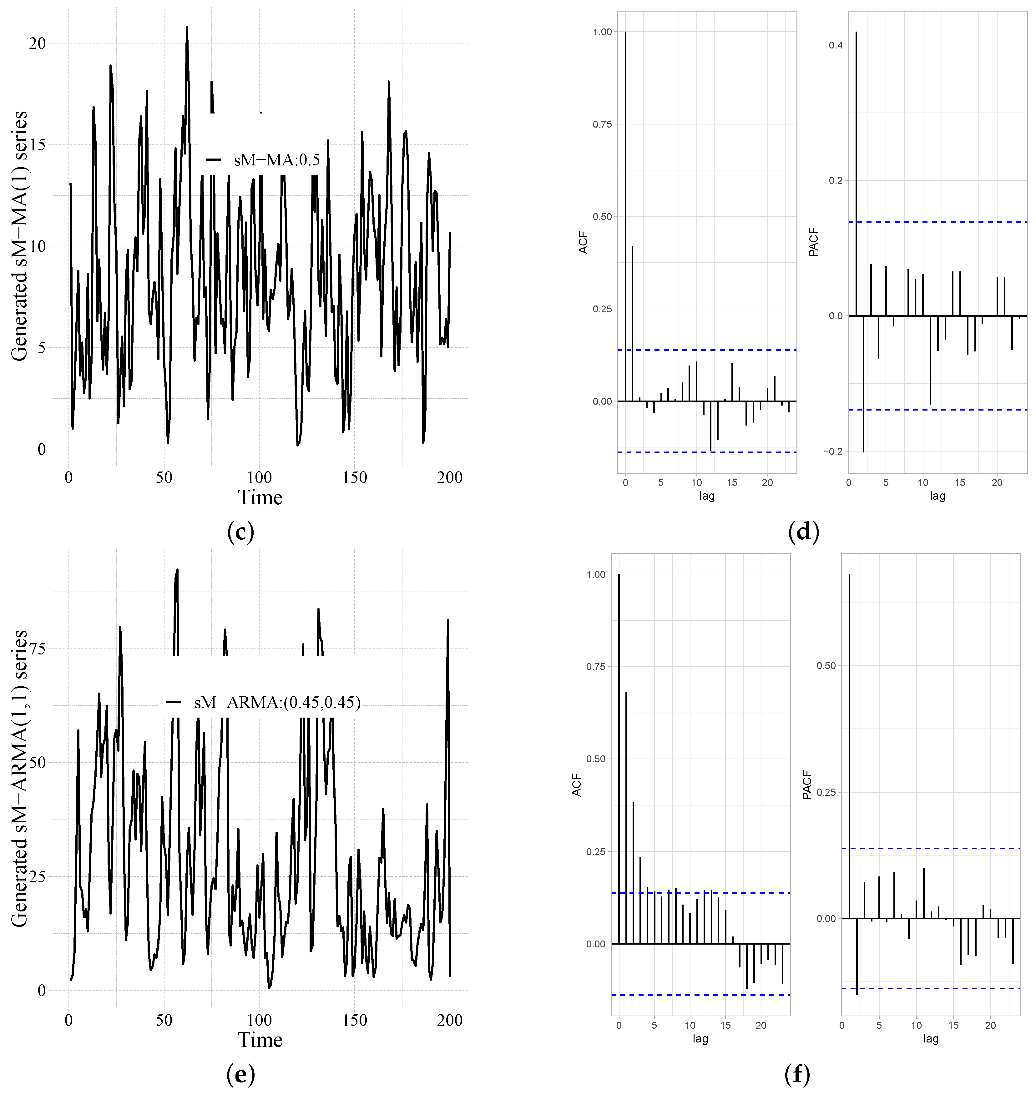
- the AR(1) process has a cut at the first lag of the partial autocorrelation function (PACF), while its autocorrelation function (ACF) experiences exponential or senoidal decrease;
- the MA(1) process has a cut at the first lag of ACF, while its PACF experiences exponential or senoidal decrease;
- the ARMA(1,1) process does not have clearly defined cuts.
2.2. Estimation
2.3. Forecasting
3. Numerical Results and Applications
3.1. Simulation Study
3.2. Application to Real-Life Data
4. Conclusions
Author Contributions
Funding
Data Availability Statement
Acknowledgments
Conflicts of Interest
Appendix A. Derivation of Score Function Components
Appendix B. Derivation of FIM
References
- Bollerslev, T. Generalized autoregressive conditional heteroskedasticity. J. Econom. 1986, 31, 307–327. [Google Scholar] [CrossRef]
- Tsay, R. Analysis of Financial Time Series; Wiley Series in Probability and Statistics; Wiley: Hoboken, NJ, USA, 2005. [Google Scholar]
- Machiwal, D.; Jha, M. Hydrologic Time Series Analysis: Theory and Practice; Springer Netherlands: Dordrecht, The Netherlands, 2011. [Google Scholar]
- Almeida-Junior, P.M.; Nascimento, A.D.C. ARMA process for speckled data. J. Stat. Comput. Simul. 2021, 91, 3125–3153. [Google Scholar] [CrossRef]
- Brockwell, P.J.; Davis, R.A. Stationary time series. In Time Series: Theory and Methods; Springer: New York, NY, USA, 1991; pp. 1–41. [Google Scholar]
- Chuang, M.D.; Yu, G.H. Order series method for forecasting non-Gaussian time series. J. Forecast. 2007, 26, 239–250. [Google Scholar] [CrossRef]
- Tiku, M.L.; Wong, W.K.; Vaughan, D.C.; Bian, G. Time series models in non-normal situations: Symmetric Innovations. J. Time Ser. Anal. 2000, 21, 571–596. [Google Scholar] [CrossRef]
- Benjamin, M.A.; Rigby, R.A.; Stasinopoulos, D.M. Generalized autoregressive moving average models. J. Am. Stat. Assoc. 2003, 98, 214–223. [Google Scholar] [CrossRef]
- Rocha, A.V.; Cribari-Neto, F. Beta autoregressive moving average models. Test 2009, 18, 529–545. [Google Scholar] [CrossRef]
- Bayer, F.M.; Bayer, D.M.; Pumi, G. Kumaraswamy autoregressive moving average models for double bounded environmental data. J. Hydrol. 2017, 555, 385–396. [Google Scholar] [CrossRef]
- Weiß, C.H.; Kim, H.Y. Binomial AR(1) processes: Moments, cumulants, and estimation. Statistics 2013, 47, 494–510. [Google Scholar] [CrossRef]
- Weiß, C.H. Integer-valued autoregressive models for counts showing underdispersion. J. Appl. Stat. 2013, 40, 1931–1948. [Google Scholar] [CrossRef]
- Lewis, P.; McKenzie, E.; Hugus, D.K. Gamma processes. Commun. Stat. Stoch. Model. 1989, 5, 1–30. [Google Scholar] [CrossRef]
- Jose, K.K.; Thomas, M.M. Generalized Laplacian distributions and autoregressive processes. Commun. Stat. Theory Methods 2011, 40, 4263–4277. [Google Scholar] [CrossRef]
- Bondon, P. Estimation of autoregressive models with epsilon-skew-normal innovations. J. Multivar. Anal. 2009, 100, 1761–1776. [Google Scholar] [CrossRef]
- Jodrá, P.; Jiménez-Gamero, M.D.; Alba-Fernández, M.V. On the Muth distribution. Math. Model. Anal. 2015, 20, 291–310. [Google Scholar] [CrossRef]
- Sardon, J.P. Prévisions de mortalité et vieillissement démographique. Gerontol. Soc. 1996, 19, 117–136. [Google Scholar] [CrossRef]
- Muth, J.E. The Theory and Applications of Reliability; Academic Press, Inc.: New York, NY, USA, 1977; Volume 2, pp. 401–435. [Google Scholar]
- Osterrieder, J.; Lorenz, J. A statistical risk assessment of bitcoin and its extreme tail behavior. Ann. Financ. Econ. 2017, 12, 1750003. [Google Scholar] [CrossRef]
- Anderson, S.; Branch, T.; Cooper, A.; Dulvy, N. Black-swan events in animal populations. Proc. Natl. Acad. Sci. USA 2017, 114, 3252–3257. [Google Scholar] [CrossRef]
- Biçer, C.; Bakouch, H.S.; Biçer, H.D. Inference on parameters of a geometric process with scaled Muth distribution. Fluct. Noise Lett. 2021, 20, 2150006. [Google Scholar] [CrossRef]
- Zheng, T.; Xiao, H.; Chen, R. Generalized ARMA models with martingale difference errors. J. Econom. 2015, 189, 492–506. [Google Scholar] [CrossRef]
- Scher, V.T.; Cribari-Neto, F.; Pumi, G.; Bayer, F.M. Goodness-of-fit tests for β-ARMA hydrological time series modeling. Environmetrics 2020, 31, e2607. [Google Scholar] [CrossRef]
- Woodard, D.B.; Matteson, D.S.; Henderson, S.G. Stationarity of generalized autoregressive moving average models. Electron. J. Stat. 2011, 5, 800–828. [Google Scholar] [CrossRef]
- Brockwell, P.; Davis, R. Time Series: Theory and Methods; Springer Series in Statistics; Springer: New York, NY, USA, 2009. [Google Scholar]
- Alizadeh, S.; Brandt, M.W.; Diebold, F.X. Range-based estimation of stochastic volatility models. J. Financ. 2002, 57, 1047–1091. [Google Scholar] [CrossRef]
- Chiang, M.H.; Wang, L.M. Volatility contagion: A range-based volatility approach. J. Econom. 2011, 165, 175–189. [Google Scholar] [CrossRef]
- Chen, C.; Twycross, J.; Garibaldi, J.M. A new accuracy measure based on bounded relative error for time series forecasting. PLoS ONE 2017, 12, e0174202. [Google Scholar] [CrossRef] [PubMed]
- Hyndman, R.; Koehler, A.; Ord, J.; Snyder, R. Forecasting with Exponential Smoothing: The State Space Approach; Springer Series in Statistics; Springer: Berlin/Heidelberg, Germany, 2008. [Google Scholar]


| link | N | MSE | MSE | MSE | MSE | ||||
|---|---|---|---|---|---|---|---|---|---|
| 49 | 0.559 | 0.493 | 0.508 | 0.992 | 0.068 | 0.074 | 0.074 | 0.218 | |
| 121 | 0.525 | 0.500 | 0.499 | 0.994 | 0.062 | 0.066 | 0.067 | 0.197 | |
| 400 | 0.507 | 0.499 | 0.502 | 0.996 | 0.063 | 0.063 | 0.064 | 0.190 | |
| 49 | 0.562 | 0.485 | 0.516 | 1.012 | 0.065 | 0.087 | 0.071 | 0.242 | |
| 121 | 0.523 | 0.502 | 0.506 | 0.999 | 0.065 | 0.069 | 0.065 | 0.203 | |
| 400 | 0.507 | 0.499 | 0.502 | 1.001 | 0.063 | 0.065 | 0.062 | 0.190 | |
| 49 | 0.556 | 0.510 | 0.497 | 0.977 | 0.0715 | 0.064 | 0.071 | 0.183 | |
| 121 | 0.521 | 0.502 | 0.498 | 0.995 | 0.065 | 0.064 | 0.066 | 0.189 | |
| 400 | 0.508 | 0.499 | 0.501 | 0.999 | 0.061 | 0.063 | 0.064 | 0.189 | |
| 49 | 0.197 | 0.470 | 0.523 | 0.980 | 0.226 | 0.123 | 0.116 | 0.372 | |
| 121 | 0.138 | 0.492 | 0.506 | 0.984 | 0.257 | 0.111 | 0.107 | 0.330 | |
| 400 | 0.113 | 0.496 | 0.503 | 0.997 | 0.274 | 0.103 | 0.104 | 0.331 | |
| 49 | 0.187 | 0.476 | 0.516 | 1.015 | 0.235 | 0.147 | 0.122 | 0.400 | |
| 121 | 0.133 | 0.492 | 0.507 | 1.001 | 0.265 | 0.117 | 0.105 | 0.342 | |
| 400 | 0.109 | 0.499 | 0.501 | 1.001 | 0.278 | 0.105 | 0.103 | 0.332 | |
| 49 | 0.193 | 0.502 | 0.494 | 0.989 | 0.229 | 0.110 | 0.111 | 0.338 | |
| 121 | 0.135 | 0.494 | 0.500 | 1.008 | 0.262 | 0.101 | 0.107 | 0.346 | |
| 400 | 0.111 | 0.498 | 0.499 | 1.003 | 0.275 | 0.104 | 0.103 | 0.334 |
| link | N | MSE | MSE | MSE | |||
|---|---|---|---|---|---|---|---|
| 49 | 0.532 | 0.481 | 1.011 | 0.091 | 0.098 | 0.196 | |
| 121 | 0.520 | 0.495 | 1.003 | 0.084 | 0.087 | 0.177 | |
| 400 | 0.504 | 0.498 | 1.001 | 0.082 | 0.084 | 0.167 | |
| 49 | 0.538 | 0.4777 | 1.028 | 0.088 | 0.106 | 0.219 | |
| 121 | 0.514 | 0.495 | 1.004 | 0.085 | 0.089 | 0.182 | |
| 400 | 0.506 | 0.498 | 1.002 | 0.084 | 0.085 | 0.171 | |
| 49 | 0.539 | 0.501 | 0.996 | 0.088 | 0.086 | 0.173 | |
| 121 | 0.509 | 0.499 | 1.000 | 0.088 | 0.084 | 0.171 | |
| 400 | 0.503 | 0.500 | 0.999 | 0.084 | 0.083 | 0.168 | |
| 49 | 0.168 | 0.472 | 1.007 | 0.285 | 0.150 | 0.384 | |
| 121 | 0.130 | 0.489 | 1.001 | 0.304 | 0.141 | 0.366 | |
| 400 | 0.107 | 0.498 | 1.001 | 0.318 | 0.140 | 0.358 | |
| 49 | 0.172 | 0.462 | 1.049 | 0.284 | 0.172 | 0.459 | |
| 121 | 0.128 | 0.481 | 1.023 | 0.306 | 0.143 | 0.392 | |
| 400 | 0.107 | 0.494 | 1.007 | 0.319 | 0.138 | 0.363 | |
| 49 | 0.171 | 0.494 | 1.007 | 0.281 | 0.137 | 0.369 | |
| 121 | 0.125 | 0.497 | 1.003 | 0.308 | 0.139 | 0.362 | |
| 400 | 0.110 | 0.497 | 1.006 | 0.318 | 0.138 | 0.360 |
| Median | Mean | SD | CV% | ||||
|---|---|---|---|---|---|---|---|
| 0.03407 | 0.07992 | 0.11732 | 0.15441 | 0.1877139 | 121.5685% | 0.16666 | 2.78590 |
| Models | / | |||
|---|---|---|---|---|
| sMuth-AR(1) | 0.2740048 | 0.8126926 | - | −0.2844197 |
| (0.03448416) | (0.06260973) | - | (0.13345582) | |
| sMuth–ARMA(1,1) | 0.30364612 | 0.93275200 | −0.25855030 | −0.06818648 |
| (0.03622131) | (0.05476766) | (0.08794887) | (0.11136618) | |
| Gaussian-AR(1) | 0.4138 | 0.1541 | - | 0.02926 |
| (0.0475) | (0.0152) | - | (0.002130622) |
| Models | MAE | MAPE | MASE |
|---|---|---|---|
| sMuth–ARMA(1,1) | 0.06575188 | 0.51026805 | 0.93168377 |
| sMuth-AR(1) | 0.06625323 | 0.51411739 | 0.93878780 |
| ETS | 0.06938751 | 0.56646631 | 0.98319957 |
| Gaussian-AR(1) | 0.06983971 | 0.60868836 | 0.98960701 |
Disclaimer/Publisher’s Note: The statements, opinions and data contained in all publications are solely those of the individual author(s) and contributor(s) and not of MDPI and/or the editor(s). MDPI and/or the editor(s) disclaim responsibility for any injury to people or property resulting from any ideas, methods, instructions or products referred to in the content. |
© 2023 by the authors. Licensee MDPI, Basel, Switzerland. This article is an open access article distributed under the terms and conditions of the Creative Commons Attribution (CC BY) license (https://creativecommons.org/licenses/by/4.0/).
Share and Cite
Nascimento, A.D.C.; Lima, M.C.S.; Bakouch, H.; Qarmalah, N. Scaled Muth–ARMA Process Applied to Finance Market. Mathematics 2023, 11, 1908. https://doi.org/10.3390/math11081908
Nascimento ADC, Lima MCS, Bakouch H, Qarmalah N. Scaled Muth–ARMA Process Applied to Finance Market. Mathematics. 2023; 11(8):1908. https://doi.org/10.3390/math11081908
Chicago/Turabian StyleNascimento, Abraão D. C., Maria C. S. Lima, Hassan Bakouch, and Najla Qarmalah. 2023. "Scaled Muth–ARMA Process Applied to Finance Market" Mathematics 11, no. 8: 1908. https://doi.org/10.3390/math11081908
APA StyleNascimento, A. D. C., Lima, M. C. S., Bakouch, H., & Qarmalah, N. (2023). Scaled Muth–ARMA Process Applied to Finance Market. Mathematics, 11(8), 1908. https://doi.org/10.3390/math11081908


