Observability of Discrete-Time Two-Time-Scale Multi-Agent Systems with Heterogeneous Features under Leader-Based Architecture

Abstract

This paper investigates the observability of discrete-time two-time-scale multi-agent systems with heterogeneous features under leader–follower architecture. First, a singular perturbation difference model for the discussed system is established based on consensus agreement. Second, to eliminate the numerical ill-posed problem that may arise from the singularly perturbed small parameter that distinguishes different time scales in the observability analysis, the order of the system model is reduced using the boundary layer theory of the singular perturbation system to obtain a slow-time-scale subsystem and a fast-time-scale subsystem. Then, based on the matrix theory, some algebraic and graphical features that guarantee the observability of the system are obtained. Finally, the validity of the theoretical results is verified by a numerical example.

1. Introduction

In the past decade, the distributed cooperative control of multi-agent systems (MASs) has been widely studied in the fields of science and engineering. Many research results have emerged on issues such as consensus [1,2], stabilizability [3], controllability [4] and so on [5,6]. Observability has received increasing attention as a fundamental and important topic for cooperative control of MASs. It is well known that in the actual industrial process, due to the limitation of measuring equipment, some system states are difficult to measure directly, but the system output can reflect the system state to a certain extent. The observability of MASs is concerned with whether the state at a certain time can be determined by observing the measured output signal within a certain period, that is, whether the state of the system can be observed or estimated from the outside.

Tanner [7] first considered controllability as well as observability for MASs in 2004 and obtained an algebraic criterion for controllability in the context of leader–follower architectures utilizing eigenvalues and eigenvectors of Laplacian matrices. Sundara et al. [8] studied the problem of structural observability over finite fields. In 2013, Liu et al. [9] published a study on the observability of complex systems, which studied the minimum sensor required for observing a complex system. Lozan et al. [10] analyzed the observability of MASs with chain topology, cyclic topology and their combination. Sabattini [11] proposed a decentralized interaction rule to ensure the observability of networked systems with time-varying topologies and showed that connection maintenance and random selection of edge rights are key concepts to ensure the observability of the system. Liu et al. [12] studied the observability of first-order, second-order and higher-order leader-based MASs with fixed topology and obtained observability conditions for the corresponding systems. Tian et al. [13] investigated the observability of switching MASs consisting of continuous-time subsystems and discrete-time subsystems.

Most of the existing research on the observability of MAS are based on the premise that the agents constituting the system are of a single type, which is far from sufficient to cover the situation as it actually exists. Zelazo et al. [14] studied the observability of network systems with homogeneous and heterogeneous dynamics and concluded that network systems that are always unobservable under homogeneous conditions can be observable or unobservable under heterogeneous conditions according to the structure of individual agent dynamics. Tian et al. [15] studied the observability of heterogeneous MASs composed of two types of agents and where different types of agents have different and switching topologies of information interactions. Based on the set of controllable states and the system matrix corresponding to all possible topologies, the corresponding criteria of observability were obtained.

In general, complex actual systems often contain different time scales, and this is also true in actual MAS. That is to say, the actual situation is not in line with all the above research results, which show that the agents constituting a MAS may work on the same time scale. For example, in the field of robotics, the dynamics of a flexible manipulator consist of two main time scales: macroscopic rigid motion and microscopic flexible vibration [16]. The existence of small parameters in the system models constructed in this case that distinguish between different time scales has led to numerical ill-posed problems when using conventional methods for observability analysis. With the deepening of scientific research, researchers become increasingly eager to explore the inherent scientific nature of complex natural phenomena, and the topic of exploring the impact of time scales has also received some researchers’ attention. Posfai [17] investigated the problem of controlling multilayer and multi-time-scale networks with one-to-one interlayer coupling. Su [18] investigated the controllability of first-order two-time-scale MASs. Then, Long [19,20,21] investigated the controllability of second-order two-time-scale MASs in continuous time and discrete time and considered the group controllability problem of first-order MASs in combination with the situation that groups are often divided to perform different tasks in actual MASs. In [22], Long analyzed the controllability of heterogeneous two-time-scale MASs.

Currently, the observability theory of MASs on a single-time scale is relatively well developed, but the observability problem of MASs on a two-time scale is rarely discussed. Different from classical linear time-invariant systems (LTIs), MASs are affected by many factors, such as the dynamics of each agent, the communication topology between agents, the control law, and the system dimension, which make the study of observability of MASs present new characteristics and theoretical difficulties. Further consideration of the impact of a two-time-scale feature on the observability of MASs is an even more challenging research task; however, there is still a gap in the research on this challenging but important task. The aim of this paper is to study the observability of MAS with a two-time-scale feature, while taking into account the influence of individual heterogeneity of agents based on a leader–follower architecture, which is a powerful supplement to the existing research results on MASs. The main contributions of this paper are summarized as follows. (i) This paper proposes research on the observability of MASs with a two-time scale for the first time, which is challenging because the traditional research methods of observability cannot be directly used here, and it is also pioneering. The heterogeneity of the individuals constituting the MASs is also considered, which brings the study closer to reality. (ii) A model for the study of the observability of MASs with a two-time scale and heterogeneous features is developed, and the steps of model reduction using the boundary layer method of singular perturbation system theory are elaborated to provide ideas for future research on this kind of problem. (iii) Based on the matrix theory, the observability analysis is carried out, and some operable observability criteria are obtained.

The organization of this paper is as follows: Section 1 reviews some mathematical preparatory knowledge. Section 2 details the motivation of the research, specifically including model introduction, modeling approach and preliminary model collation. In Section 3, reduced order modeling is carried out based on the boundary layer method of the singular perturbation system theory, and the slow-time-scale subsystem and fast-time-scale subsystem are obtained. Section 4 specifies the observability analysis. Numerical simulation results are presented in Section 5. Conclusions of the paper are presented in Section 6.

2. Mathematical Preliminaries

Here are some lemmas that will be used for the rest of this paper.

Lemma 1 

([23]). For a constant matrix E with compatible dimensions, if all eigenvalues β of $e^E$ satisfy $\left|\beta \left(e^E\right)\right|<1$, then

$$\epsilon \sum _{q=0}^{\left[1/\epsilon \right]-1}{\left(I+\epsilon E\right)}^{\left[1/\epsilon \right]-1-q}={\int }_0^1{e}^{Et}dt+O\left(\epsilon \right),$$

(1)

can be obtained when $\epsilon \to 0$.

Lemma 2 

([23]). For a constant matrix E with compatible dimensions, if all eigenvalues β of $e^E$ satisfy $\left|\beta \left(e^E\right)\right|<1$, then

$${\left(I+\epsilon E\right)}^{\left[1/\epsilon \right]}\sim e^E+O\left(\epsilon \right),$$

(2)

can be obtained when $\epsilon \to 0$.

Lemma 3 

([24]). For real matrices ${\Xi }_1$, ${\Xi }_2$ and ${\Xi }_3$ satisfying the conditions ${\Xi }_1={\Xi }_1^T$ and ${\Xi }_2={\Xi }_2^T>0$, it follows that the linear matrix inequality ${\Xi }_1+{\Xi }_3^T{\Xi }_2^{-1}{\Xi }_3<0$ holds if and only if

$$\left[\begin{array}{cc}{\Xi }_1& {\Xi }_3^T\\ {\Xi }_3& -{\Xi }_2\end{array}\right]<0.$$

(3)

Note that in the next narrative, $\mathbb{R}$ denotes the set of real numbers, I denotes a unit matrix with compatible dimensions, and 0 denotes either a zero element, a zero vector or a zero matrix with compatible dimensions. A weighted directed graph $\mathcal{G}=\left(\mathcal{V},\mathcal{E}\right)$ is made up of nodes $\mathcal{V}=\left\{v_1,v_2,\dots ,v_n\right\}$ and the edges $\mathcal{E}\subseteq \mathcal{V}\times \mathcal{V}$. For the edge $\left(v_i,v_j\right)$, $a_{ij}$ represents the coupling weight between $v_i$ and $v_j$. The number of edges pointing away from a node $v_i$ is the outgoing degree of the node $v_i$, while the number of edges pointing into it is its incoming degree. The neighborhood ${\mathcal{N}}_i=\left\{v_j\in \mathcal{V}:\left(v_i,v_j\right)\in \mathcal{E}\right\}$ of a node $v_i$ is the set of all nodes adjacent to it. $A=\left[a_{ij}\right]$ and $L=\left[l_{ij}\right]$ denote the adjacency matrix and the Laplacian matrix of the graph $\mathcal{G}$, respectively, where $l_{ij}=\left\{\begin{array}{c}-a_{ij},i\ne j\\ {\displaystyle \sum _{j\in N_i}}{a}_{ij},i=j\end{array}\right.$ and $i,j\in \left\{1,2,\dots ,n\right\}$.

3. Motivation

A discrete-time MAS considered in this paper is based on a leader–follower architecture and is considered to have two different time scales, while also considering that the dynamics of the agents that make up the MAS are not unique in type, that is, some are first-order agents and others are second-order agents. To demonstrate more clearly the object under discussion, a legend of such a system model is given through Figure 1.

As can be seen in Figure 1, the agents can be divided into four parts, namely, a cluster of first-order follower agents $\left(G\left(f_1\right)\right)$, a cluster of first-order leader agents $\left(G\left(l_1\right)\right)$, a cluster of second-order follower agents $\left(G\left(f_2\right)\right)$ and a cluster of second-order leader agents $\left(G\left(l_2\right)\right)$. The red vertices as well as the green vertices are used to distinguish between the leader role or the follower role assumed by the different agents.

To facilitate the mathematical description, we use $e_1\stackrel{\Delta }{=}\left\{i_1,i_2,\dots ,i_a,i_{a+1},\dots ,i_{a+b}\right\}$ and $e_2\stackrel{\Delta }{=}\left\{i_{a+b+1},i_{a+b+2},\dots ,i_{a+b+c},i_{a+b+c+1},\dots ,i_{a+b+c+d}\right\}$ to represent the index of first-order and second-order agents, respectively. The index set of leader agent is $V_l=\left\{i_{a+1},i_{a+2},\dots ,\right.\left.i_{a+b},i_{a+b+c+1},\dots ,i_{a+b+c+d}\right\}$, and the remaining set $V_f=\left\{i_1,i_2,\dots ,i_a,i_{a+b+1},\dots ,i_{a+b+c}\right\}$ is the index of the follower agent.

The information interactions between the agents are presented in the form of linked edges in Figure 1 and can also be described mathematically by the following matrix L.

$$S=\left[\begin{array}{cccc}{S}_{f_1{f}_1}& S_{f_1{l}_1}& S_{f_1{f}_2}& S_{f_1{l}_2}\\ S_{l_1{f}_1}& S_{l_1{l}_1}& S_{l_1{f}_2}& S_{l_1{l}_2}\\ S_{f_2{f}_1}& S_{f_2{l}_1}& S_{f_2{f}_2}& S_{f_2{l}_2}\\ S_{l_2{f}_1}& S_{l_2{l}_1}& S_{l_2{f}_2}& S_{l_2{l}_2}\end{array}\right]=\left[\begin{array}{cccc}{S}_{11}& S_{12}& S_{13}& S_{14}\\ S_{21}& S_{22}& S_{23}& S_{24}\\ S_{31}& S_{32}& S_{33}& S_{34}\\ S_{41}& S_{42}& S_{43}& S_{44}\end{array}\right].$$

(4)

Due to the consideration of the two-time-scale feature, and taking into account the practical situation, each agent is considered here to operate on two different time scales simultaneously. In this way, for the first-order agent $j\in e_1$, there are position information $x_j\in {\mathbb{R}}^{n_x}$ and $s_j\in {\mathbb{R}}^{n_s}$ on the slow- and fast-time-scale, and for the second-order agent $j\in e_2$, there are not only position and speed information $x_j\in {\mathbb{R}}^{n_x}$ and $d_j\in {\mathbb{R}}^{n_x}$ on the slow-time scale, but also position and speed information $s_j\in {\mathbb{R}}^{n_s}$ and $w_j\in {\mathbb{R}}^{n_s}$ on the fast-time scale. With the above setting, the model of the MAS discussed in this paper can be described as

$$\begin{array}{cc}\hfill & \left\{\begin{array}{c}{x}_j\left(k+1\right)=\left(I+\epsilon A\right)x_j\left(k\right)+\epsilon B_1{u}_j\left(k\right),\hfill \\ s_j\left(k+1\right)=\left(I+A\right)s_j\left(k\right)+B_2{u}_j\left(k\right),j\in e_1,\hfill \end{array}\right.\hfill \end{array}$$

(5)

$$\begin{array}{cc}\hfill & \left\{\begin{array}{c}{x}_j\left(k+1\right)=\left(I+\epsilon A\right)x_j\left(k\right)+\epsilon d_j\left(k\right),\hfill \\ d_j\left(k+1\right)=\left(I+\epsilon A\right)d_j\left(k\right)+\epsilon B_1{u}_j\left(k\right),\hfill \\ s_j\left(k+1\right)=\left(I+A\right)s_j\left(k\right)+w_j\left(k\right),\hfill \\ w_j\left(k+1\right)=\left(I+A\right)w_j\left(k\right)+B_2{u}_j\left(k\right),j\in e_2,\hfill \end{array}\right.\hfill \end{array}$$

(6)

where $B_1\in {\mathbb{R}}^{n_x\times q}$ and $B_2\in {\mathbb{R}}^{n_s\times q}$ are corresponding input matrices on two different time scales, $u_j\left(k\right)\in {\mathbb{R}}^q$ is the control inputs.

For the MAS (5) and (6), the designed communication protocol is

$$u_j\left(k\right)\left\{\begin{array}{c}\mathrm{(7)}& F_1{\displaystyle \sum _{o\in N_j}}{a}_{jo}\left(x_o\left(k\right)-x_j\left(k\right)\right)+F_2{\displaystyle \sum _{o\in N_j}}{a}_{jo}\left(s_o\left(k\right)-s_j\left(k\right)\right),j\in e_1,\hfill F_1{\displaystyle \sum _{o\in N_j}}{a}_{jo}\left(x_o\left(k\right)-x_j\left(k\right)\right)+F_2{\displaystyle \sum _{o\in N_j}}{a}_{jo}\left(s_o\left(k\right)-s_j\left(k\right)\right)\hfill \\ \mathrm{(8)}& +E_1{\displaystyle \sum _{o\in N_j}}{a}_{jo}\left(d_o\left(k\right)-d_j\left(k\right)\right)+E_2{\displaystyle \sum _{o\in N_j}}{a}_{jo}\left(w_o\left(k\right)-w_j\left(k\right)\right),j\in e_2,\hfill \end{array}\right.$$

in conjunction with the consensus protocol, where $F_1\in {\mathbb{R}}^{q\times n_x}$ and $F_2\in {\mathbb{R}}^{q\times n_s}$ denote the position state coupling matrix, while $E_1\in {\mathbb{R}}^{q\times n_x}$ and $E_2\in {\mathbb{R}}^{q\times n_s}$ are the speed state coupling matrix.

Organizing the Equations (5)–(8) above and noting that $x_{f1}={\left(x_1^T,x_2^T,...,x_a^T\right)}^T\in {\mathbb{R}}^{a{n}_x}$, $x_{l1}={\left(x_{a+1}^T,x_{a+2}^T,...,x_{a+b}^T\right)}^T\in {\mathbb{R}}^{b{n}_x}$, $s_{f1}={\left(s_1^T,s_2^T,...,s_a^T\right)}^T\in {\mathbb{R}}^{a{n}_s}$, $s_{l1}={\left(s_{a+1}^T,s_{a+2}^T,...,s_{a+b}^T\right)}^T$$\in {\mathbb{R}}^{b{n}_s}$, $x_{f2}={\left(x_{a+b+1}^T,x_{a+b+2}^T,...,x_{a+b+c}^T\right)}^T\in {\mathbb{R}}^{c{n}_x}$, $x_{l2}={\left(x_{a+b+c+1}^T,x_{a+b+c+2}^T,...,x_{a+b+c+d}^T\right)}^T\in {\mathbb{R}}^{d{n}_x}$, $s_{f2}={\left(s_{a+b+1}^T,s_{a+b+2}^T,...,s_{a+b+c}^T\right)}^T\in {\mathbb{R}}^{c{n}_s}$, $s_{l2}={\left(s_{a+b+c+1}^T,s_{a+b+c+2}^T,...,s_{a+b+c+d}^T\right)}^T\in {\mathbb{R}}^{d{n}_s}$, $d_{f2}={\left(d_{a+b+1}^T,d_{a+b+2}^T,...,d_{a+b+c}^T\right)}^T\in {\mathbb{R}}^{c{n}_x}$, $d_{l2}={\left(d_{a+b+c+1}^T,d_{a+b+c+2}^T,...,d_{a+b+c+d}^T\right)}^T\in {\mathbb{R}}^{d{n}_x}$, $w_{f2}={\left(w_{a+b+1}^T,w_{a+b+2}^T,...,w_{a+b+c}^T\right)}^T\in {\mathbb{R}}^{c{n}_s}$, $w_{l2}={\left(w_{a+b+c+1}^T,w_{a+b+c+2}^T,...,w_{a+b+c+d}^T\right)}^T\in {\mathbb{R}}^{d{n}_s}$ gives

$$\begin{array}{cc}\hfill \left[\begin{array}{c}{x}_{f1}\left(k+1\right)\\ x_{f2}\left(k+1\right)\\ d_{f2}\left(k+1\right)\\ s_{f1}\left(k+1\right)\\ s_{f2}\left(k+1\right)\\ w_{f2}\left(k+1\right)\end{array}\right]& =\left[\begin{array}{cccccc}I+\epsilon \left(I\otimes A\right)+\epsilon {\Omega }_{11}& \epsilon {\Omega }_{12}& 0& \epsilon {\Omega }_{14}& \epsilon {\Omega }_{15}& 0\\ 0& I+\epsilon \left(I\otimes A\right)& \epsilon I& 0& 0& 0\\ \epsilon {\Omega }_{31}& \epsilon {\Omega }_{32}& I+\epsilon \left(I\otimes A\right)+\epsilon {\Omega }_{33}& \epsilon {\Omega }_{34}& \epsilon {\Omega }_{35}& \epsilon {\Omega }_{36}\\ {\Omega }_{41}& {\Omega }_{42}& 0& I+\left(I\otimes A\right)+{\Omega }_{44}& {\Omega }_{45}& 0\\ 0& 0& 0& 0& I+\left(I\otimes A\right)& I\\ {\Omega }_{61}& {\Omega }_{62}& {\Omega }_{63}& {\Omega }_{64}& {\Omega }_{65}& I+\left(I\otimes A\right)+{\Omega }_{66}\end{array}\right]\hfill \\ \hfill & \times \left[\begin{array}{c}{x}_{f1}\left(k\right)\\ x_{f2}\left(k\right)\\ d_{f2}\left(k\right)\\ s_{f1}\left(k\right)\\ s_{f2}\left(k\right)\\ w_{f2}\left(k\right)\end{array}\right]+\left[\begin{array}{cccccc}\epsilon {\vartheta }_{11}& \epsilon {\vartheta }_{12}& 0& \epsilon {\vartheta }_{14}& \epsilon {\vartheta }_{15}& 0\\ 0& 0& 0& 0& 0& 0\\ \epsilon {\vartheta }_{31}& \epsilon {\vartheta }_{32}& \epsilon {\vartheta }_{33}& \epsilon {\vartheta }_{34}& \epsilon {\vartheta }_{35}& \epsilon {\vartheta }_{36}\\ {\vartheta }_{41}& {\vartheta }_{42}& 0& {\vartheta }_{44}& {\vartheta }_{45}& 0\\ 0& 0& 0& 0& 0& 0\\ {\vartheta }_{61}& {\vartheta }_{62}& {\vartheta }_{63}& {\vartheta }_{64}& {\vartheta }_{65}& {\vartheta }_{66}\end{array}\right]\times \left[\begin{array}{c}{x}_{l1}\left(k\right)\\ x_{l2}\left(k\right)\\ d_{l2}\left(k\right)\\ s_{l1}\left(k\right)\\ s_{l2}\left(k\right)\\ w_{l2}\left(k\right)\end{array}\right],\hfill \end{array}$$

(9)

where ${\Omega }_{11}=-S_{11}\otimes B_1{F}_1$, ${\Omega }_{12}=-S_{13}\otimes B_1{F}_1$, ${\Omega }_{14}=-S_{11}\otimes B_1{F}_2$, ${\Omega }_{15}=-S_{13}\otimes B_1{F}_2$, ${\Omega }_{31}=-S_{31}\otimes B_1{F}_1$, ${\Omega }_{32}=-S_{33}\otimes B_1{F}_1$, ${\Omega }_{33}=-S_{33}\otimes B_1{E}_1$, ${\Omega }_{34}=-S_{31}\otimes B_1{F}_2$, ${\Omega }_{35}=-S_{33}\otimes B_1{F}_2$, ${\Omega }_{36}=-S_{33}\otimes B_1{E}_2$, ${\Omega }_{41}=-S_{11}\otimes B_2{F}_1$, ${\Omega }_{42}=-S_{13}\otimes B_2{F}_1$, ${\Omega }_{44}=-S_{11}\otimes B_2{F}_2$, ${\Omega }_{45}=-S_{13}\otimes B_2{F}_2$, ${\Omega }_{61}=-S_{31}\otimes B_2{F}_1$, ${\Omega }_{62}=-S_{33}\otimes B_2{F}_1$, ${\Omega }_{63}=-S_{33}\otimes B_2{E}_1$, ${\Omega }_{64}=-S_{31}\otimes B_2{F}_2$, ${\Omega }_{65}=-S_{33}\otimes B_2{F}_2$, ${\Omega }_{66}=-S_{33}\otimes B_2{E}_2$, ${\vartheta }_{11}=-S_{12}\otimes B_1{F}_1$, ${\vartheta }_{12}=-S_{14}\otimes B_1{F}_1$, ${\vartheta }_{14}=-S_{12}\otimes B_1{F}_2$, ${\vartheta }_{15}=-S_{14}\otimes B_1{F}_2$, ${\vartheta }_{31}=-S_{32}\otimes B_1{F}_1$, ${\vartheta }_{32}=-S_{34}\otimes B_1{F}_1$, ${\vartheta }_{33}=-S_{34}\otimes B_1{E}_1$, ${\vartheta }_{34}=-S_{32}\otimes B_1{F}_2$, ${\vartheta }_{35}=-S_{34}\otimes B_1{F}_2$, ${\vartheta }_{36}=-S_{34}\otimes B_1{E}_2$, ${\vartheta }_{41}=-S_{12}\otimes B_2{F}_1$, ${\vartheta }_{42}=-S_{14}\otimes B_2{F}_1$, ${\vartheta }_{44}=-S_{12}\otimes B_2{F}_2$, ${\vartheta }_{45}=-S_{14}\otimes B_2{F}_2$, ${\vartheta }_{61}=-S_{32}\otimes B_2{F}_1$, ${\vartheta }_{62}=-S_{34}\otimes B_2{F}_1$, ${\vartheta }_{63}=-S_{34}\otimes B_2{E}_1$, ${\vartheta }_{64}=-S_{32}\otimes B_2{F}_2$, ${\vartheta }_{65}=-S_{34}\otimes B_2{F}_2$, ${\vartheta }_{66}=-S_{34}\otimes B_2{E}_2$.

Then, let $r_1={\left(x_{f1}^T,x_{f2}^T,d_{f2}^T\right)}^T\in {\mathbb{R}}^{a{n}_x+2c{n}_x}$, $r_2={\left(s_{f1}^T,s_{f2}^T,w_{f2}^T\right)}^T\in {\mathbb{R}}^{a{n}_s+2c{n}_s}$ and $u={\left(x_{l1}^T,x_{l2}^T,d_{l2}^T,s_{l1}^T,s_{l2}^T,w_{l2}^T\right)}^T\in {\mathbb{R}}^{\left(b+2d\right)n_x+\left(b+2d\right)n_s}$ to obtain

$$\left\{\begin{array}{}\mathrm{(10)}& r_1\left(k+1\right)=\left(I+\epsilon \left(I\otimes A\right)+\epsilon {\phi }_{11}\right)r_1\left(k\right)+\epsilon {\phi }_{12}{r}_2\left(k\right)+\epsilon {\varphi }_{1}u\left(k\right),\mathrm{(11)}& r_2\left(k+1\right)={\phi }_{21}{r}_1\left(k\right)+\left(I+\left(I\otimes A\right)+{\phi }_{22}\right)r_2\left(k\right)+{\varphi }_{2}u\left(k\right),\end{array}\right.$$

where ${\varphi }_1=\left[\begin{array}{cccccc}{\vartheta }_{11}& {\vartheta }_{12}& 0& {\vartheta }_{14}& {\vartheta }_{15}& 0\\ 0& 0& 0& 0& 0& 0\\ {\vartheta }_{31}& {\vartheta }_{32}& {\vartheta }_{33}& {\vartheta }_{34}& {\vartheta }_{35}& {\vartheta }_{36}\end{array}\right]$, ${\varphi }_2=\left[\begin{array}{cccccc}{\vartheta }_{41}& {\vartheta }_{42}& 0& {\vartheta }_{44}& {\vartheta }_{45}& 0\\ 0& 0& 0& 0& 0& 0\\ {\vartheta }_{61}& {\vartheta }_{62}& {\vartheta }_{63}& {\vartheta }_{64}& {\vartheta }_{65}& {\vartheta }_{66}\end{array}\right]$, ${\phi }_{11}=\left[\begin{array}{ccc}{\Omega }_{11}& {\Omega }_{12}& 0\\ 0& 0& I\\ {\Omega }_{31}& {\Omega }_{32}& {\Omega }_{33}\end{array}\right]$, ${\phi }_{12}=\left[\begin{array}{ccc}{\Omega }_{14}& {\Omega }_{15}& 0\\ 0& 0& 0\\ {\Omega }_{34}& {\Omega }_{35}& {\Omega }_{36}\end{array}\right]$, ${\phi }_{21}=\left[\begin{array}{ccc}{\Omega }_{41}& {\Omega }_{42}& 0\\ 0& 0& 0\\ {\Omega }_{61}& {\Omega }_{62}& {\Omega }_{63}\end{array}\right]$, ${\phi }_{22}=\left[\begin{array}{ccc}{\Omega }_{44}& {\Omega }_{45}& 0\\ 0& 0& I\\ {\Omega }_{64}& {\Omega }_{65}& {\Omega }_{66}\end{array}\right]$.

For the MAS depicted in Figure 1, the states of the system are often difficult to measure directly due to the limitations of the measurement equipment in the actual control process, and what can be measured is usually some output signals. The so-called observability of the MAS mentioned in the Introduction means that the state of the whole MAS can be observed through only a few agents as far as possible. This is similar to the reason for leading the whole MAS with a minimum number of leaders. In this paper, it is assumed that leaders can measure the status information of their neighbors and exchange the obtained information with other leaders. According to this, we take the output vector measured by the leaders as the output of the system.

Accordingly, for Equations (10) and (11),

$$y\left(k\right)={\varphi }_1^T{r}_1\left(k\right)+{\varphi }_2^T{r}_2\left(k\right),$$

(12)

is chosen as the output.

Therefore, the complete dynamic equation for the MAS considered in this paper is

$$\left\{\begin{array}{c}{r}_1\left(k+1\right)=\left(I+\epsilon \left(I\otimes A\right)+\epsilon {\phi }_{11}\right)r_1\left(k\right)+\epsilon {\phi }_{12}{r}_2\left(k\right)+\epsilon {\varphi }_{1}u\left(k\right),\hfill \\ r_2\left(k+1\right)={\phi }_{21}{r}_1\left(k\right)+\left(I+I\otimes A+{\phi }_{22}\right)r_2\left(k\right)+{\varphi }_{2}u\left(k\right),\hfill \\ y\left(k\right)={\varphi }_1^T{r}_1\left(k\right)+{\varphi }_2^T{r}_2\left(k\right),\hfill \end{array}\right.$$

(13)

which can be regarded as the classical singularly perturbed system equation, and it should be noted that $y\left(k\right)\in {\mathbb{R}}^{\left(b+2d\right)n_x+\left(b+2d\right)n_s}$.

4. Reduced-Order Modeling

System (13) is referred to as a singularly perturbed system in view of the existence of the singularly perturbed parameter $\epsilon$ that distinguishes different time scales. If the conventional observability theory is used for the observability analysis of the above system, it will lead to the ill-posed problems. In this paper, a reduced-order decomposition of System (13) is first performed based on the boundary layer correction method [25,26,27,28] of the singularly perturbed system.

Consider first the slow-time-scale subsystem, at which point the state of the fast-time-scale subsystem is considered to have reached a steady state, and it is reasonable to assume that matrix ${\phi }_{22}$ is invertible, such that Equation (11) can be written as

$$r_{2s}\left(k\right)={\phi }_{21}{r}_{1s}\left(k\right)+\left(I+\left(I\otimes A\right)+{\phi }_{22}\right)r_{2s}\left(k\right)+{\varphi }_2{u}_s\left(k\right).$$

(14)

Thus,

$$r_{2s}\left(k\right)=-{\left(I\otimes A+{\phi }_{22}\right)}^{-1}{\phi }_{21}{r}_{1s}\left(k\right)-{\left(I\otimes A+{\phi }_{22}\right)}^{-1}{\varphi }_2{u}_s\left(k\right).$$

(15)

Substituting (15) into (10) gives

$$r_{1s}\left(k+1\right)=\left(I+\epsilon \left(I\otimes A+{\phi }_{11}-{\phi }_{12}{\left(I\otimes A+{\phi }_{22}\right)}^{-1}{\phi }_{21}\right)\right)r_{1s}\left(k\right)+\epsilon \left({\varphi }_1-{\phi }_{12}{\left(I\otimes A+{\phi }_{22}\right)}^{-1}{\varphi }_2\right)u_s\left(k\right).$$

(16)

Let ${\phi }_s=I\otimes A+{\phi }_{11}-{\phi }_{12}{\left(I\otimes A+{\phi }_{22}\right)}^{-1}{\phi }_{21}$, ${\varphi }_s={\varphi }_1-{\phi }_{12}{\left(I\otimes A+{\phi }_{22}\right)}^{-1}{\varphi }_2$, then we have

$$r_{1s}\left(k+1\right)=\left(I+\epsilon {\phi }_s\right)r_{1s}\left(k\right)+\epsilon {\varphi }_s{u}_s\left(k\right).$$

(17)

The time scale of the slow-time-scale subsystem is denoted by h and defined by

$$k=\left[h/\epsilon \right],h=1,2,...$$

(18)

In addition, the control input signal of the slow-time-scale subsystem remains unchanged during $h\left[1/\epsilon \right]\le k<\left(h+1\right)\left[1/\epsilon \right]$ and can be expressed as $u_s\left(k\right)={\widehat{u}}_s\left(h\left[1/\epsilon \right]\right)$. Accordingly,

$$\begin{array}{cc}\hfill r_{1s}\left(h\left[1/\epsilon \right]+1\right)& =\left(I+\epsilon {\phi }_s\right)r_{1s}\left(h\left[1/\epsilon \right]\right)+\epsilon {\varphi }_s{\widehat{u}}_s\left(h\left[1/\epsilon \right]\right),\hfill \\ \hfill r_{1s}\left(h\left[1/\epsilon \right]+2\right)& ={\left(I+\epsilon {\phi }_s\right)}^2{r}_{1s}\left(h\left[1/\epsilon \right]\right)+\epsilon \left(I+\epsilon {\phi }_s\right){\varphi }_s{\widehat{u}}_s\left(h\left[1/\epsilon \right]\right)+\epsilon {\varphi }_s{\widehat{u}}_s\left(h\left[1/\epsilon \right]\right),\hfill \\ \hfill & ...\hfill \\ \hfill r_{1s}\left(\left(h+1\right)\left[1/\epsilon \right]\right)& ={\left(I+\epsilon {\phi }_s\right)}^{\left[1/\epsilon \right]}{r}_{1s}\left(h\left[1/\epsilon \right]\right)+\epsilon \sum _{q=0}^{\left[1/\epsilon \right]-1}{\left(I+\epsilon {\phi }_s\right)}^{\left[1/\epsilon \right]-1-q}{\varphi }_s{\widehat{u}}_s\left(h\left[1/\epsilon \right]\right)\hfill \end{array}$$

(19)

can be derived. When the value of $\left[1/\epsilon \right]$ is large enough, according to Lemmas 1 and 2, and let ${\widehat{\phi }}_s\stackrel{\Delta }{=}{e}^{{\phi }_s}$ and ${\widehat{\varphi }}_s\stackrel{\Delta }{=}{\int }_0^1{e}^{{\phi }_{s}t}dt{\varphi }_s$, there is

$$r_{1s}\left(\left(h+1\right)\left[1/\epsilon \right]\right)=\left({\widehat{\phi }}_s+O\left(\epsilon \right)\right)r_{1s}\left(h\left[1/\epsilon \right]\right)+\left({\widehat{\varphi }}_s+O\left(\epsilon \right)\right){\widehat{u}}_s\left(h\left[1/\epsilon \right]\right).$$

(20)

Denote ${\widehat{r}}_{1s}\left(h\right)=r_{1s}\left(h\left[1/\epsilon \right]\right)$ and the equation for the reduced order slow-time-scale subsystem can be obtained as

$${\widehat{r}}_{1s}\left(h+1\right)={\widehat{\phi }}_s{\widehat{r}}_{1s}\left(h\right)+{\widehat{\varphi }}_s{\widehat{u}}_s\left(h\right)$$

(21)

provided that infinitesimal terms are neglected.

The state variable $r_1\left(k\right)$ can be considered to remain invariant when considering the fast-time-scale subsystem.

$$\begin{array}{c}\hfill r_2\left(k+1\right)-r_{2s}\left(k+1\right)={\phi }_{21}{r}_1\left(k\right)+\left(I+\left(I\otimes A\right)+{\phi }_{22}\right)r_2\left(k\right)+{\varphi }_{2}u\left(k\right)-{\phi }_{21}{r}_{1s}\left(k\right)+\left(I+\left(I\otimes A\right)+{\phi }_{22}\right)r_{2s}\left(k\right)+{\varphi }_2{u}_s\left(k\right)\end{array}$$

(22)

can be obtained by subtracting Equation (14) from Equation (11). By defining $r_{2f}\left(k\right)\stackrel{\Delta }{=}{r}_2\left(k\right)-r_{2s}\left(k\right)$, $u_f\left(k\right)\stackrel{\Delta }{=}u\left(k\right)-u_s\left(k\right)$ and combining $r_1\left(k\right)=r_{1s}\left(k\right)$, there is

$$r_{2f}\left(k+1\right)=\left(I+I\otimes A+{\phi }_{22}\right)r_{2f}\left(k\right)+{\varphi }_2{u}_f\left(k\right).$$

(23)

Noting that ${\phi }_f=I+I\otimes A+{\phi }_{22}$ and ${\varphi }_f={\varphi }_2$, it follows that

$$r_{2f}\left(k+1\right)={\phi }_f{r}_{2f}\left(k\right)+{\varphi }_f{u}_f\left(k\right),$$

(24)

which is the state equation of the fast-time-scale subsystem.

Because $y\left(k\right)={\varphi }_1^T{r}_1\left(k\right)+{\varphi }_2^T{r}_2\left(k\right)={\varphi }_1^T{r}_{1s}\left(k\right)+{\varphi }_2^T\left(r_{2f}\left(k\right)+r_{2s}\left(k\right)\right)$, there is

$$\left\{\begin{array}{c}{y}_s\left(k\right)={\varphi }_1^T{r}_{1s}\left(k\right)+{\varphi }_2^T{r}_{2s}\left(k\right)\hfill \\ y_f\left(k\right)={\varphi }_2^T{r}_{2f}\left(k\right).\hfill \end{array}\right.$$

(25)

By substituting Equation (15) into (26),

$$y_s\left(k\right)=\left({\varphi }_1^T-{\varphi }_2^T{\left(I\otimes A+{\phi }_{22}\right)}^{-1}{\phi }_{21}\right)r_{1s}\left(k\right)-{\varphi }_2^T{\left(I\otimes A+{\phi }_{22}\right)}^{-1}{\varphi }_2{u}_s\left(k\right),$$

(26)

and

$$y_f\left(k\right)={\varphi }_2^T{r}_{2f}\left(k\right)={\varphi }_f^T{r}_{2f}\left(k\right)$$

(27)

are obtained.

To sum up,

$$\left\{\begin{array}{c}{\widehat{r}}_{1s}\left(h+1\right)={\widehat{\phi }}_s{\widehat{r}}_{1s}\left(h\right)+{\widehat{\varphi }}_s{\widehat{u}}_s\left(h\right)\hfill \\ {\widehat{y}}_s\left(h\right)=\left({\varphi }_1^T-{\varphi }_2^T{\left(I\otimes A+{\phi }_{22}\right)}^{-1}{\phi }_{21}\right){\widehat{r}}_{1s}\left(h\right)-{\varphi }_2^T{\left(I\otimes A+{\phi }_{22}\right)}^{-1}{\varphi }_2{\widehat{u}}_s\left(h\right)\hfill \end{array}\right.$$

(28)

is the reduced-order slow-time-scale subsystem and

$$\left\{\begin{array}{c}{r}_{2f}\left(k+1\right)={\phi }_f{r}_{2f}\left(k\right)+{\varphi }_f{u}_f\left(k\right)\hfill \\ y_f\left(k\right)={\varphi }_f^T{r}_{2f}\left(k\right)\hfill \end{array}\right.$$

(29)

is the reduced-order fast-time-scale subsystem, where ${\widehat{y}}_s\left(h\right)\stackrel{\Delta }{=}{y}_s\left(h\left[1/\epsilon \right]\right)$ and ${\widehat{u}}_s\left(h\right)\stackrel{\Delta }{=}{u}_s\left(h\left[1/\epsilon \right]\right)$. Let $C_0={\varphi }_1^T-{\varphi }_2^T{\left(I\otimes A+{\phi }_{22}\right)}^{-1}{\phi }_{21}$, $D_0=-{\varphi }_2^T{\left(I\otimes A+{\phi }_{22}\right)}^{-1}{\varphi }_2$ and $C_1={\varphi }_f^T$, then

$$\left\{\begin{array}{c}{\widehat{r}}_{1s}\left(h+1\right)={\widehat{\phi }}_s{\widehat{r}}_{1s}\left(h\right)+{\widehat{\varphi }}_s{\widehat{u}}_s\left(h\right)\hfill \\ {\widehat{y}}_s\left(h\right)=C_0{\widehat{r}}_{1s}\left(h\right)+D_0{\widehat{u}}_s\left(h\right),\hfill \end{array}\right.$$

(30)

$$\left\{\begin{array}{c}{r}_{2f}\left(k+1\right)={\phi }_f{r}_{2f}\left(k\right)+{\varphi }_f{u}_f\left(k\right)\hfill \\ y_f\left(k\right)=C_1{r}_{2f}\left(k\right).\hfill \end{array}\right.$$

(31)

5. Observability Analysis

Definition 1. 

The states $r_{10}$ and $r_{20}$ of System (13) are said to be unobservable for the given initial states $r_1\left(k_0\right)=r_{10}$ as well as $r_2\left(k_0\right)=r_{20}$, if $y\left(k\right)=0$ holds for any $k\in \left\{k_0,k_1,\cdots ,k_f\right\}$, where $k_f$ is a finite time and satisfies $k_f>k_0$. System (13) is said to be observable if it has no unobservable states.

Lemma 4. 

For System (13), if and only if

$$\begin{array}{cc}\hfill rank{\left[\begin{array}{cccc}{C}_0^T& {\widehat{\phi }}_s^T{C}_0^T& \cdots & {\left({\widehat{\phi }}_s^T\right)}^{\left(a{n}_x+2c{n}_x-1\right)}{C}_0^T\end{array}\right]}^T& =a{n}_x+2c{n}_x,\hfill \end{array}$$

(32)

$$\begin{array}{cc}\hfill rank{\left[\begin{array}{cccc}{\varphi }_f& {\phi }_f^T{\varphi }_f& \cdots & {\left({\phi }_f^T\right)}^{\left(a{n}_s+2c{n}_s-1\right)}{\varphi }_f\end{array}\right]}^T& =a{n}_s+2c{n}_s,\hfill \end{array}$$

(33)

there exists some ${\epsilon }^{*}>0$ such that System (13) is completely observable for all $\epsilon \in \left(\left.0,{\epsilon }^{*}\right]\right.$.

Proof. 

The proof process of Lemma 4 can be omitted because of Definition 1 and Kalman observability rank criterion [29]. □

Theorem 1. 

For System (13), the following propositions are equivalent.

1.

System (13) is observable.

2.

For any $s\in \mathbb{R}$ and $v\in \mathbb{R}$, there are matrices $\left[\begin{array}{c}sI-{\widehat{\phi }}_s\\ C_0\end{array}\right]$ and $\left[\begin{array}{c}vI-{\phi }_f\\ {\varphi }_f^T\end{array}\right]$ with full rank.

3.

No non-zero right eigenvector α of the matrix ${\widehat{\phi }}_s$ is orthogonal to all rows of $C_0$, that is, for all eigenvalues λ of the matrix ${\widehat{\phi }}_s$, if both ${\widehat{\phi }}_s\alpha =\lambda \alpha$ and $C_0\alpha =0$ are true, then the right eigenvector α must be a zero vector. In addition, the matrix ${\phi }_f$ has no non-zero right eigenvectors p orthogonal to all rows of ${\varphi }_f^T$, i.e., for all eigenvalues γ of the matrix ${\phi }_f$, the right eigenvector p must be zero if ${\phi }_{f}p=\gamma p$ and ${\varphi }_f^{T}p=0$ both hold.

Proof of Theorem 1 (2). 

Necessity: Assume that neither matrix $\left[\begin{array}{c}sI-{\widehat{\phi }}_s\\ C_0\end{array}\right]$ nor matrix $\left[\begin{array}{c}vI-{\phi }_f\\ {\varphi }_f^T\end{array}\right]$ is a full rank matrix, that is, the column vectors of the matrix $\left[\begin{array}{c}sI-{\widehat{\phi }}_s\\ C_0\end{array}\right]$ are linearly correlated, as are the column vectors of the matrix $\left[\begin{array}{c}vI-{\phi }_f\\ {\varphi }_f^T\end{array}\right]$. Therefore, there exists non-zero vectors $\rho$ and $\gamma$ such that

$$\left[\begin{array}{c}sI-{\widehat{\phi }}_s\\ C_0\end{array}\right]\rho =0,\left[\begin{array}{c}vI-{\phi }_f\\ {\varphi }_f^T\end{array}\right]\gamma =0.$$

(34)

Thus,

$$\left(sI-{\widehat{\phi }}_s\right)\rho =0,C_0\rho =0,\left(vI-{\phi }_f\right)\gamma =0,{\varphi }_f^T\gamma =0.$$

(35)

This in turn gives

$$\left\{\begin{array}{c}{C}_0\rho =0,\begin{array}{cc}& C_0{\widehat{\phi }}_s\rho =0\end{array},\begin{array}{cc}\cdots ,& C_0{\widehat{\phi }}_s^{\left(a{n}_x+2c{n}_x-1\right)}\rho =\end{array}0,\hfill \\ {\varphi }_f^T\gamma =0,\begin{array}{cc}& {\varphi }_f^T{\phi }_f\gamma =0\end{array},\begin{array}{cc}\cdots ,& {\varphi }_f^T{{\phi }_f}^{\left(a{n}_s+2c{n}_s-1\right)}\gamma =\end{array}0.\hfill \end{array}\right.$$

(36)

Then,

$$\begin{array}{c}{\left[\begin{array}{cccc}{C}_0^T& {\widehat{\phi }}_s^T{C}_0^T& \cdots & {\left({\widehat{\phi }}_s^T\right)}^{\left(a{n}_x+2c{n}_x-1\right)}{C}_0^T\end{array}\right]}^T\rho =0,\hfill \\ {\left[\begin{array}{cccc}{\varphi }_f& {\phi }_f^T{\varphi }_f& \cdots & {\left({\phi }_f^T\right)}^{\left(a{n}_s+2c{n}_s-1\right)}{\varphi }_f\end{array}\right]}^T\gamma =0.\hfill \end{array}$$

(37)

can be obtained by sorting. Since the vectors $\rho$ and $\gamma$ are both non-zero vectors, according to Lemma 4, System (13) is unobservable.

Sufficiency: Assuming that System (13) is unobservable, and that it follows from Lemma 4 that $rank{\left[\begin{array}{cccc}{C}_0^T& {\widehat{\phi }}_s^T{C}_0^T& \cdots & {\left({\widehat{\phi }}_s^T\right)}^{\left(a{n}_x+2c{n}_x-1\right)}{C}_0^T\end{array}\right]}^T<a{n}_x+2c{n}_x$ and $a{n}_s+2c{n}_s>rank$${\left[\begin{array}{cccc}{\varphi }_f& {\phi }_f^T{\varphi }_f& \cdots & {\left({\phi }_f^T\right)}^{\left(a{n}_s+2c{n}_s-1\right)}{\varphi }_f\end{array}\right]}^T$, then for the matrices ${\widehat{\phi }}_s$ and ${\phi }_f$ there exist eigenvectors $\rho$ and $\gamma$ about eigenvalues ${\lambda }_{\mathrm{s}}$ and ${\lambda }_f$, respectively, satisfying

$$\begin{array}{c}{\left[\begin{array}{cccc}{C}_0^T& {\widehat{\phi }}_s^T{C}_0^T& \cdots & {\left({\widehat{\phi }}_s^T\right)}^{\left(a{n}_x+2c{n}_x-1\right)}{C}_0^T\end{array}\right]}^T\rho =0,\hfill \\ {\left[\begin{array}{cccc}{\varphi }_f& {\phi }_f^T{\varphi }_f& \cdots & {\left({\phi }_f^T\right)}^{\left(a{n}_s+2c{n}_s-1\right)}{\varphi }_f\end{array}\right]}^T\gamma =0.\hfill \end{array}$$

(38)

Further,

$$C_0\rho =0,C_0{\widehat{\phi }}_s\rho =0,{\varphi }_f^T\gamma =0,{\varphi }_f^T{\phi }_f\gamma =0.$$

(39)

In addition, since

$${\widehat{\phi }}_s\rho ={\lambda }_{\mathrm{s}}\rho ,{\phi }_f\gamma ={\lambda }_f\gamma ,$$

(40)

it follows that $rank\left[\begin{array}{c}{\lambda }_{\mathrm{s}}I-{\widehat{\phi }}_s\\ C_0\end{array}\right]<a{n}_x+2c{n}_x$ and $rank\left[\begin{array}{c}{\lambda }_{f}I-{\phi }_f\\ {\varphi }_f^T\end{array}\right]<a{n}_s+2c{n}_s$. Thus far, it is clear that the sufficiency is proved. □

Proof of Theorem 1 (3). 

Necessity: Suppose there exist non-zero vectors $\alpha$ and p satisfying ${\widehat{\phi }}_s\alpha =\lambda \alpha$, $C_0\alpha =0$, ${\phi }_{f}p=\gamma p$ and ${\varphi }_f^{T}p=0$. It is obvious that

$$\begin{array}{c}{C}_0\alpha =0,C_0{\widehat{\phi }}_s\alpha =\lambda C_0\alpha =0,C_0{{\widehat{\phi }}_s}^2\alpha =\lambda C_0{\widehat{\phi }}_s\alpha =0,\cdots ,C_0{{\widehat{\phi }}_s}^{\left(a{n}_x+2c{n}_x-1\right)}\alpha =0,\hfill \\ {\varphi }_f^{T}p=0,{\varphi }_f^T{\phi }_{f}p=\gamma {\varphi }_f^{T}p=0,{\varphi }_f^T{{\phi }_f}^{2}p=\gamma {\varphi }_f^T{\phi }_{f}p=0,\cdots ,C_0{{\widehat{\phi }}_s}^{\left(a{n}_s+2c{n}_s-1\right)}\alpha =0.\hfill \end{array}$$

(41)

Therefore,

$$\begin{array}{c}{\left[\begin{array}{cccc}{C}_0^T& {\widehat{\phi }}_s^T{C}_0^T& \cdots & {\left({\widehat{\phi }}_s^T\right)}^{\left(a{n}_x+2c{n}_x-1\right)}{C}_0^T\end{array}\right]}^T\alpha =0,\hfill \\ {\left[\begin{array}{cccc}{\varphi }_f& {\phi }_f^T{\varphi }_f& \cdots & {\left({\phi }_f^T\right)}^{\left(a{n}_s+2c{n}_s-1\right)}{\varphi }_f\end{array}\right]}^{T}p=0.\hfill \end{array}$$

(42)

Since both $\alpha$ and p are non-zero vectors, there is $rank{\left[\begin{array}{cc}{C}_0^T& {\widehat{\phi }}_s^T{C}_0^T\cdots {\left({\widehat{\phi }}_s^T\right)}^{\left(a{n}_x+2c{n}_x-1\right)}{C}_0^T\end{array}\right]}^T$ $<a{n}_x+2c{n}_x$ and $rank{\left[\begin{array}{cccc}{\varphi }_f& {\phi }_f^T{\varphi }_f& \cdots & {\left({\phi }_f^T\right)}^{\left(a{n}_s+2c{n}_s-1\right)}{\varphi }_f\end{array}\right]}^T<a{n}_s+2c{n}_s$, and according to Lemma 4, System (13) is unobservable.

Sufficiency: Reference can be made to the proof of the sufficiency of Theorem 1 (2). □

Theorem 2. 

System (13) is observable if both of the following conditions are satisfied.

1.

The eigenvalues of the matrix ${\widehat{\phi }}_s$ are different, and the eigenvalues of the matrix ${\phi }_f$ are also different.

2.

All row vectors of matrix $C_0$ are not simultaneously orthogonal to at least one eigenvector of matrix ${\widehat{\phi }}_s$, and all row vectors of matrix ${\varphi }_f^T$ are not simultaneously orthogonal to at least one eigenvector of ${\phi }_f$.

Proof. 

Suppose that the eigenvalues of the matrix ${\widehat{\phi }}_s$ are all different, then ${\widehat{\phi }}_s=UD{U}^{-1}$, where $D=diag\left(\begin{array}{cccc}{\lambda }_1& {\lambda }_2& \cdots & {\lambda }_{a{n}_x+2c{n}_x}\end{array}\right)$, ${\lambda }_i\left(i=1,\dots ,a{n}_x+2c{n}_x\right)$ is the eigenvalue of the matrix ${\widehat{\phi }}_s$ and U is composed of the eigenvectors of ${\widehat{\phi }}_s$. The corresponding observability matrix is

$$Q_0=\left[\begin{array}{c}{C}_0\\ C_0{\widehat{\phi }}_s\\ ⋮\\ C_0{{\widehat{\phi }}_s}^{\left(a{n}_x+2c{n}_x-1\right)}\end{array}\right]=\left[\begin{array}{c}{C}_{0}U\\ C_{0}UD\\ ⋮\\ C_{0}U{D}^{\left(a{n}_x+2c{n}_x-1\right)}\end{array}\right]U^{-1}.$$

(43)

Since the matrix $U^{-1}$ is non-singular, let ${\tilde{Q}}_0=$ $[U^T{C}_0^T,D^T{U}^T{C}_0^T,\cdots ,{\left(D^T\right)}^{\left(a{n}_x+2c{n}_x-1\right)}{U}^T$ $C_0^T{]}^T$, then $rank{Q}_0=rank{\tilde{Q}}_0$. The expansion of $C_{0}U$ is expressed as

$$C_{0}U={\left[\begin{array}{cccc}{\eta }_1^T& {\eta }_2^T& \cdots & {\eta }_{\left(\left(b+2d\right)n_x+\left(b+2d\right)n_s\right)}^T\end{array}\right]}^T,$$

(44)

where ${\eta }_i=\left[\begin{array}{cccc}{\eta }_{i1}& {\eta }_{i2}& \cdots & {\eta }_{i\left(a{n}_x+2c{n}_x\right)}\end{array}\right]\in {\mathbb{R}}^{1\times \left(a{n}_x+2c{n}_x\right)}$; thus,

$$\begin{array}{cc}\hfill rank{\tilde{Q}}_0& =rank\left[\begin{array}{c}{\left[\begin{array}{cccc}{\eta }_1^T& {\eta }_2^T& \cdots & {\eta }_{\left(\left(b+2d\right)n_x+\left(b+2d\right)n_s\right)}^T\end{array}\right]}^T\\ {\left[\begin{array}{cccc}{\eta }_1^T& {\eta }_2^T& \cdots & {\eta }_{\left(\left(b+2d\right)n_x+\left(b+2d\right)n_s\right)}^T\end{array}\right]}^{T}D\\ ⋮\\ {\left[\begin{array}{cccc}{\eta }_1^T& {\eta }_2^T& \cdots & {\eta }_{\left(\left(b+2d\right)n_x+\left(b+2d\right)n_s\right)}^T\end{array}\right]}^T{D}^{\left(a{n}_x+2c{n}_x-1\right)}\end{array}\right]\hfill \\ \hfill & =rank\left[\begin{array}{c}{\eta }_1\\ {\eta }_{1}D\\ ⋮\\ {\eta }_1{D}^{\left(a{n}_x+2c{n}_x-1\right)}\\ {\eta }_2\\ {\eta }_{2}D\\ ⋮\\ {\eta }_2{D}^{\left(a{n}_x+2c{n}_x-1\right)}\\ ⋮\\ {\eta }_{{}_{\left(\left(b+2d\right)n_x+\left(b+2d\right)n_s\right)}}\\ {\eta }_{{}_{\left(\left(b+2d\right)n_x+\left(b+2d\right)n_s\right)}}D\\ ⋮\\ {\eta }_{\left(\left(b+2d\right)n_x+\left(b+2d\right)n_s\right)}{D}^{\left(a{n}_x+2c{n}_x-1\right)}\end{array}\right].\hfill \end{array}$$

(45)

can be obtained.

Since ${\eta }_{1}D=\left[\begin{array}{cccc}{\eta }_{11}& {\eta }_{12}& \cdots & {\eta }_{1\left(a{n}_x+2c{n}_x\right)}\end{array}\right]diag\left(\begin{array}{cccc}{\lambda }_1& {\lambda }_2& \cdots & {\lambda }_{a{n}_x+2c{n}_x}\end{array}\right)=$ $\left[\begin{array}{cccc}{\lambda }_1{\eta }_{11}& {\lambda }_2{\eta }_{12}& \cdots & {\lambda }_{a{n}_x+2c{n}_x}{\eta }_{1\left(a{n}_x+2c{n}_x\right)}\end{array}\right]$, and so on, we obtain

$$\begin{array}{c}\hfill \left[\begin{array}{c}{\eta }_1\\ {\eta }_{1}D\\ ⋮\\ {\eta }_1{D}^{\left(a{n}_x+2c{n}_x-1\right)}\end{array}\right]=\left[\begin{array}{cccc}1& 1& \cdots & 1\\ {\lambda }_1& {\lambda }_2& \cdots & {\lambda }_{\left(a{n}_x+2c{n}_x\right)}\\ ⋮& ⋮& \ddots & ⋮\\ {\lambda }_1^{\left(a{n}_x+2c{n}_x-1\right)}& {\lambda }_2^{\left(a{n}_x+2c{n}_x-1\right)}& \cdots & {\lambda }_{\left(a{n}_x+2c{n}_x\right)}^{\left(a{n}_x+2c{n}_x-1\right)}\end{array}\right]\left[\begin{array}{cccc}{\eta }_{11}& & & \\ & {\eta }_{12}& & \\ & & \ddots & \\ & & & {\eta }_{1\left(a{n}_x+2c{n}_x\right)}\end{array}\right].\end{array}$$

(46)

Let $H=\left[\begin{array}{cccc}1& 1& \cdots & 1\\ {\lambda }_1& {\lambda }_2& \cdots & {\lambda }_{\left(a{n}_x+2c{n}_x\right)}\\ ⋮& ⋮& \ddots & ⋮\\ {\lambda }_1^{\left(a{n}_x+2c{n}_x-1\right)}& {\lambda }_2^{\left(a{n}_x+2c{n}_x-1\right)}& \cdots & {\lambda }_{\left(a{n}_x+2c{n}_x\right)}^{\left(a{n}_x+2c{n}_x-1\right)}\end{array}\right]$, which is a Vandermonde matrix. Therefore,

$$rank{\tilde{Q}}_0=rank\left[\begin{array}{c}H\left[\begin{array}{cccc}{\eta }_{11}& & & \\ & {\eta }_{12}& & \\ & & \ddots & \\ & & & {\eta }_{1\left(a{n}_x+2c{n}_x\right)}\end{array}\right]\\ H\left[\begin{array}{cccc}{\eta }_{21}& & & \\ & {\eta }_{22}& & \\ & & \ddots & \\ & & & {\eta }_{2\left(a{n}_x+2c{n}_x\right)}\end{array}\right]\\ ⋮\\ H\left[\begin{array}{cccc}{\eta }_{\left(\left(b+2d\right)n_x+\left(b+2d\right)n_s\right)\times 1}& & & \\ & {\eta }_{\left(\left(b+2d\right)n_x+\left(b+2d\right)n_s\right)\times 2}& & \\ & & \ddots & \\ & & & {\eta }_{\left(\left(b+2d\right)n_x+\left(b+2d\right)n_s\right)\times \left(a{n}_x+2c{n}_x\right)}\end{array}\right]\end{array}\right].$$

(47)

Let $U\stackrel{\Delta }{=}$ $[u_1,u_2,\cdots ,u_{a{n}_x+2c{n}_x}]\in {\mathbb{R}}^{\left(a{n}_x+2c{n}_x\right)\times \left(a{n}_x+2c{n}_x\right)}$ and $C_0\stackrel{\Delta }{=}$ $[p_1^T,p_2^T,\cdots ,p_{\left(b+2d\right)n_x+\left(b+2d\right)n_s}^T]\in {\mathbb{R}}^{\left(\left(b+2d\right)n_x+\left(b+2d\right)n_s\right)\times \left(a{n}_x+2c{n}_x\right)}$, where $p_i\in$ ${\mathbb{R}}^{1\times \left(a{n}_x+2c{n}_x\right)}$. If

$$\begin{array}{c}{C}_{0}U={\left[\begin{array}{cccc}{\eta }_1^T& {\eta }_2^T& \cdots & {\eta }_{\left(\left(b+2d\right)n_x+\left(b+2d\right)n_s\right)}^T\end{array}\right]}^T\hfill \\ \begin{array}{cc}& \end{array}\begin{array}{c}=\left[\begin{array}{cccc}{\eta }_{11}& {\eta }_{12}& \cdots & {\eta }_{1\left(a{n}_x+2c{n}_x\right)}\\ {\eta }_{21}& {\eta }_{22}& \cdots & {\eta }_{2\left(a{n}_x+2c{n}_x\right)}\\ ⋮& ⋮& \ddots & ⋮\\ {\eta }_{\left(\left(b+2d\right)n_x+\left(b+2d\right)n_s\right)\times 1}& {\eta }_{\left(\left(b+2d\right)n_x+\left(b+2d\right)n_s\right)\times 2}& \cdots & {\eta }_{\left(\left(b+2d\right)n_x+\left(b+2d\right)n_s\right)\times \left(a{n}_x+2c{n}_x\right)}\end{array}\right]\end{array}\hfill \\ \begin{array}{cc}& \end{array}\begin{array}{c}=\left[\begin{array}{c}{p}_1\\ p_2\\ ⋮\\ p_{\left(b+2d\right)n_x+\left(b+2d\right)n_s}\end{array}\right]\end{array}\left[\begin{array}{cccc}{u}_1& u_2& \cdots & u_{a{n}_x+2c{n}_x}\end{array}\right]\hfill \end{array},$$

(48)

then for any $i\in \left\{1,2,\dots ,\left(b+2d\right)n_x+\left(b+2d\right)n_s\right\}$ and $j\in \left\{1,2,\dots ,a{n}_x+2c{n}_x\right\}$, there is ${\eta }_{i,j}=\left(p_i,u_j\right)$. This in turn gives

$$\begin{array}{c}rank{\tilde{Q}}_0=rank\hfill \\ \left[\begin{array}{c}H\left[\begin{array}{cccc}\left(p_1,u_1\right)& & & \\ & \left(p_1,u_2\right)& & \\ & & \ddots & \\ & & & \left(p_1,u_{\left(a{n}_x+2c{n}_x\right)}\right)\end{array}\right]\\ H\left[\begin{array}{cccc}\left(p_2,u_1\right)& & & \\ & \left(p_2,u_2\right)& & \\ & & \ddots & \\ & & & \left(p_2,u_{\left(a{n}_x+2c{n}_x\right)}\right)\end{array}\right]\\ ⋮\\ H\left[\begin{array}{cccc}\left(p_{\left(\left(b+2d\right)n_x+\left(b+2d\right)n_s\right)},u_1\right)& & & \\ & \left(p_{\left(\left(b+2d\right)n_x+\left(b+2d\right)n_s\right)},u_2\right)& & \\ & & \ddots & \\ & & & \left(p_{\left(\left(b+2d\right)n_x+\left(b+2d\right)n_s\right)},u_{\left(a{n}_x+2c{n}_x\right)}\right)\end{array}\right]\end{array}\right]\hfill \end{array}.$$

(49)

Obviously, H is a full-rank matrix if all the eigenvalues of the matrix ${\widehat{\phi }}_s$ are different from each other. In addition, if all the eigenvectors $u_i$ of ${\widehat{\phi }}_s$ are not simultaneously orthogonal to at least one row of the matrix $C_0$, then at least one of the block matrices

$$\left[\begin{array}{cccc}\left(p_i,u_1\right)& & & \\ & \left(p_i,u_2\right)& & \\ & & \ddots & \\ & & & \left(p_i,u_{\left(a{n}_x+2c{n}_x\right)}\right)\end{array}\right].$$

(50)

is also full rank. Thus, the matrix ${\tilde{Q}}_0$ is column full-rank, and thus, the matrix $Q_0$ is also column full-rank. A similar proof process can be obtained with respect to the matrices ${\phi }_f$ and ${\varphi }_f^T$. In summary, and in conjunction with Lemma 4, it follows that System (13) is observable. □

Theorem 3. 

System (13) is observable if both of the following conditions are satisfied.

1.

The matrix ${\widehat{\phi }}_s$ have different eigenvalues; the matrix ${\phi }_f$ also have different eigenvalues.

2.

Each column of $C_{0}U$ has at least one non-zero element; each column of ${\varphi }_f^{T}V$ also has at least one non-zero element, where U is made up of eigenvectors of ${\widehat{\phi }}_s$, and V is made up of eigenvectors of ${\phi }_f$.

Proof. 

Suppose that the eigenvalues of the matrix ${\widehat{\phi }}_s$ are all different, then ${\widehat{\phi }}_s=UD{U}^{-1}$, where $D=diag\left(\begin{array}{cccc}{\lambda }_1& {\lambda }_2& \cdots & {\lambda }_{a{n}_x+2c{n}_x}\end{array}\right)$. The eigenvectors of ${\widehat{\phi }}_s$ form the matrix U and the eigenvalues of the matrix ${\widehat{\phi }}_s$ are expressed as ${\lambda }_i\left(i=1,\dots ,a{n}_x+2c{n}_x\right)$. The corresponding observability matrix is

$$\begin{array}{c}{Q}_0=\left[\begin{array}{c}{C}_0\\ C_0{\widehat{\phi }}_s\\ ⋮\\ C_0{{\widehat{\phi }}_s}^{\left(a{n}_x+2c{n}_x-1\right)}\end{array}\right]\hfill \\ \begin{array}{cc}& =\end{array}\left[\begin{array}{c}{C}_{0}U\\ C_{0}UD\\ ⋮\\ C_{0}U{D}^{\left(a{n}_x+2c{n}_x-1\right)}\end{array}\right]U^{-1}.\hfill \end{array}$$

(51)

Since the matrix $U^{-1}$ is non-singular, $\left|U^{-1}\right|\ne 0$, which gives

$$rank{Q}_0=rank\left[\begin{array}{c}{C}_{0}U\\ C_{0}UD\\ ⋮\\ C_{0}U{D}^{\left(a{n}_x+2c{n}_x-1\right)}\end{array}\right].$$

(52)

The matrices involved in the right-hand side of Equation (52) can again be regarded as the observability matrix of a new system whose output matrix as well as the system matrix are $C_{0}U$ and D. However, if

$$C_{0}U=\left[\begin{array}{cccc}{b}_{11}& b_{12}& \cdots & b_{1\left(a{n}_x+2c{n}_x\right)}\\ b_{21}& b_{22}& \cdots & b_{2\left(a{n}_x+2c{n}_x\right)}\\ ⋮& ⋮& \ddots & ⋮\\ b_{\left(\left(b+2d\right)n_x+\left(b+2d\right)n_s\right)\times 1}& b_{\left(\left(b+2d\right)n_x+\left(b+2d\right)n_s\right)\times 2}& \cdots & b_{\left(\left(b+2d\right)n_x+\left(b+2d\right)n_s\right)\times \left(a{n}_x+2c{n}_x\right)}\end{array}\right]$$

(53)

is defined, then

$$\begin{array}{c}rank\left[\begin{array}{c}{\lambda }_{i}I-D\\ C_{0}U\end{array}\right]=rank\hfill \\ \left[\begin{array}{cccc}{\lambda }_i-{\lambda }_1& & & \\ & {\lambda }_i-{\lambda }_2& & \\ & & \ddots & \\ & & & {\lambda }_i-{\lambda }_{a{n}_x+2c{n}_x}\\ b_{11}& b_{12}& \cdots & b_{1\left(a{n}_x+2c{n}_x\right)}\\ b_{21}& b_{22}& \cdots & b_{2\left(a{n}_x+2c{n}_x\right)}\\ ⋮& ⋮& \ddots & ⋮\\ b_{\left(\left(b+2d\right)n_x+\left(b+2d\right)n_s\right)\times 1}& b_{\left(\left(b+2d\right)n_x+\left(b+2d\right)n_s\right)\times 2}& \cdots & b_{\left(\left(b+2d\right)n_x+\left(b+2d\right)n_s\right)\times \left(a{n}_x+2c{n}_x\right)}\end{array}\right]\hfill \end{array}.$$

(54)

Thus far, the two conditions in Theorem 3 lead to

$$rank\left[\begin{array}{c}{\lambda }_{i}I-D\\ C_{0}U\end{array}\right]=a{n}_x+2c{n}_x.$$

(55)

According to Theorem 1 (2), the new system is observable, equivalent to

$$rank\left[\begin{array}{c}{C}_{0}U\\ C_{0}UD\\ ⋮\\ C_{0}U{D}^{\left(a{n}_x+2c{n}_x-1\right)}\end{array}\right]=a{n}_x+2c{n}_x.$$

(56)

Similarly, the same conclusion can be drawn with respect to matrices ${\phi }_f$ and ${\varphi }_f^T$. To sum up, according to Lemma 4, it can be concluded that system (13) is observable. □

Theorem 4. 

If the matrix

$$Q=\left[\begin{array}{cccc}{\widehat{\phi }}_s& {\widehat{\varphi }}_s& 0& 0\\ C_0& I& 0& 0\\ 0& 0& {\phi }_f& {\varphi }_f\\ 0& 0& {{\varphi }_f}^T& I\end{array}\right].$$

(57)

does not have the same eigenvalues as the previously mentioned matrices ${\widehat{\phi }}_s$, ${\phi }_f$, then the system (13) is observable.

Proof. 

Theorem 4 is equivalent to the fact that if System (13) is unobservable, then there is at least one identical eigenvalue between the matrices ${\widehat{\phi }}_s$ and Q and at least one identical eigenvalue between ${\phi }_f$ and Q. Then, it follows from Theorem 1 (3) that there exists a non-zero vector $\alpha \in {\mathbb{R}}^{\left(a+2c\right)n_x}$ such that ${\widehat{\phi }}_s\alpha =\lambda \alpha$ and $C_0\alpha =0$ holds. In addition, there exists a non-zero vector $p\in {\mathbb{R}}^{\left(a+2c\right)n_s}$ such that ${\phi }_{f}p=\mu p$ and ${\varphi }_f^{T}p=0$ both hold.

Defining a new vector ${\left[\begin{array}{cccc}{\alpha }^T& 0& 0& 0\end{array}\right]}^T$, we have

$$\begin{array}{c}Q\left[\begin{array}{c}\alpha \\ 0\\ 0\\ 0\end{array}\right]=\left[\begin{array}{cccc}{\widehat{\phi }}_s& {\widehat{\varphi }}_s& 0& 0\\ C_0& I& 0& 0\\ 0& 0& {\phi }_f& {\varphi }_f\\ 0& 0& {{\varphi }_f}^T& I\end{array}\right]\left[\begin{array}{c}\alpha \\ 0\\ 0\\ 0\end{array}\right]=\left[\begin{array}{c}\lambda \alpha \\ 0\\ 0\\ 0\end{array}\right]\begin{array}{c}=\lambda \left[\begin{array}{c}\alpha \\ 0\\ 0\\ 0\end{array}\right]\end{array}\hfill \end{array}.$$

(58)

Clearly, it follows that the matrix ${\widehat{\phi }}_s$ and the matrix Q have an identical eigenvalue.

Similarly, defining a new vector ${\left[\begin{array}{cccc}0& 0& p^T& 0\end{array}\right]}^T$, we have

$$Q\left[\begin{array}{c}0\\ 0\\ p\\ 0\end{array}\right]=\left[\begin{array}{cccc}{\widehat{\phi }}_s& {\widehat{\varphi }}_s& 0& 0\\ C_0& I& 0& 0\\ 0& 0& {\phi }_f& {\varphi }_f\\ 0& 0& {{\varphi }_f}^T& I\end{array}\right]\left[\begin{array}{c}0\\ 0\\ p\\ 0\end{array}\right]=\left[\begin{array}{c}0\\ 0\\ {\phi }_{f}p\\ {{\varphi }_f}^{T}p\end{array}\right]=\mu \left[\begin{array}{c}0\\ 0\\ p\\ 0\end{array}\right].$$

(59)

Obviously, it can be concluded that there is the same eigenvalue $\mu$ between the matrix ${\phi }_f$ and the matrix Q. To sum up, Theorem 4 is proved. □

Theorem 5. 

If System (13) is observable, then the out-degree of the cluster composed of all follower agents should be non-zero.

Proof. 

Assume that the out-degree of the cluster composed of all follower agents is zero, that is, there is no information flow from the cluster of the follower agents. Then, it is known that ${\varphi }_1^T=0$ and ${\varphi }_2^T=0$. Thus, $C_0={\varphi }_1^T-{\varphi }_2^T{\phi }_{22}^{-1}{\phi }_{21}=0$ and $C_1={\varphi }_f^T=0$. It follows that

$$rank{\left[\begin{array}{cccc}{C}_0^T& {\widehat{\phi }}_s^T{C}_0^T& \cdots & {\left({\widehat{\phi }}_s^T\right)}^{\left(a{n}_x+2c{n}_x-1\right)}{C}_0^T\end{array}\right]}^T<a{n}_x+2c{n}_x.$$

(60)

$$rank{\left[\begin{array}{cccc}{\varphi }_f& {\phi }_f^T{\varphi }_f& \cdots & {\left({\phi }_f^T\right)}^{\left(a{n}_z+2c{n}_z-1\right)}{\varphi }_f\end{array}\right]}^T<a{n}_z+2c{n}_z.$$

(61)

According to Lemma 4, the MAS (13) is unobservable. Therefore, the hypothesis does not hold, that is, if System (13) is observable, then the overall out-degree of the cluster composed of all follower agents must be non-zero. □

6. Simulation

Simulation results of a MAS consisting of five first-order agents and four second-order agents are used to illustrate the effectiveness of Lemma 4; Theorem 1–5 are valid. In this example, two and one of the first- and second-order agents act as leaders, respectively, while the rest act as followers. See Figure 2 for details, with

$$S_{11}=\left[\begin{array}{ccc}0.7& 0& -0.2\\ 0& 0.5& 0\\ 0& -0.3& 0.8\end{array}\right],S_{13}=\left[\begin{array}{ccc}0& 0& 0\\ -0.2& 0& 0\\ 0& 0& 0\end{array}\right],$$

$$S_{12}=\left[\begin{array}{cc}0& -0.5\\ -0.3& 0\\ 0& 0\end{array}\right],S_{14}=\left[\begin{array}{c}0\\ 0\\ -0.5\end{array}\right],$$

$$S_{21}=\left[\begin{array}{ccc}-0.5& 0& 0\\ 0& -1& 0\end{array}\right],S_{23}=\left[\begin{array}{ccc}0& 0& 0\\ 0& -1& 0\end{array}\right],$$

$$S_{22}=\left[\begin{array}{cc}0.5& 0\\ 0& 2\end{array}\right],S_{24}=\left[\begin{array}{c}\begin{array}{c}0\\ 0\end{array}\end{array}\right],$$

$$S_{31}=\left[\begin{array}{ccc}-0.1& -0.1& 0\\ -0.1& 0& -0.2\\ 0& 0& 0\end{array}\right],S_{33}=\left[\begin{array}{ccc}0.7& 0& -0.5\\ 0& 1.6& 0\\ 0& 0& 0.5\end{array}\right],$$

$$S_{32}=\left[\begin{array}{cc}0& 0\\ 0& -1\\ 0& 0\end{array}\right],S_{34}=\left[\begin{array}{c}0\\ -0.3\\ -0.5\end{array}\right],$$

$$S_{41}=\left[\begin{array}{ccc}0& 0& 0\end{array}\right],S_{43}=\left[\begin{array}{ccc}-0.5& 0& 0\end{array}\right],$$

$$S_{42}=\left[\begin{array}{c}\begin{array}{cc}0& 0\end{array}\end{array}\right],S_{44}=\left[\begin{array}{c}0.5\end{array}\right].$$

The values of the coefficient matrices $B_1$, $B_2$, $F_1$, $F_2$, $E_1$ and $E_2$ involved are

$$B_1=\left[\begin{array}{cc}1& 2\end{array}\right],B_2=\left[\begin{array}{cc}1& 1\end{array}\right],$$

$$F_1=\left[\begin{array}{c}1\\ 3\end{array}\right],F_2=\left[\begin{array}{c}2\\ 1\end{array}\right],E_1=\left[\begin{array}{c}2\\ 3\end{array}\right],E_2=\left[\begin{array}{c}1\\ 3\end{array}\right].$$

It can be seen from Figure 2 that $a=3$, $b=2$, $c=3$, $d=1$. Without losing generality, it is assumed that the state of each agent is one-dimensional, that is, $n_x=n_s=1$. Furthermore, take $A=\left[0.5\right]$. From the calculations, it follows that $rank$ ${\left[\begin{array}{cccc}{C}_0^T& {\widehat{\phi }}_s^T{C}_0^T& \cdots & {\left({\widehat{\phi }}_s^T\right)}^{\left(a{n}_x+2c{n}_x-1\right)}{C}_0^T\end{array}\right]}^T=9$ and $rank$ ${\left[\begin{array}{cccc}{\varphi }_f& {\phi }_f^T{\varphi }_f& \cdots & {\left({\phi }_f^T\right)}^{\left(a{n}_z+2c{n}_s-1\right)}{\varphi }_f\end{array}\right]}^T=9$, that is to say, the observability matrix is column full rank. From Lemma 4, this system is observable.

The calculation yields

$${\widehat{\phi }}_s=\left[\begin{array}{ccccccccc}1.6687& 1.107& 1.5294& 1.1591& 1& 0.9378& 1.4007& 1& 0.9229\\ 1.0701& 3.0884& 1.0216& 3.2039& 1& 0.6968& 6.6655& 1& 0.6366\\ 1.0326& 2.1619& 1.3493& 1.4824& 1& 0.8427& 2.4561& 1& 0.8074\\ 1& 1& 1& 1.6487& 1& 1& 2.7183& 1& 1\\ 1& 1& 1& 1& 1.6487& 1& 1& 2.7183& 1\\ 1& 1& 1& 1& 1& 1.6487& 1& 1& 2.7183\\ 1.0115& 0.8817& 0.9522& 0.0137& 1& 15.9982& 0.0084& 1& 21.9902\\ 1.0234& 0.7703& 1.1033& 0.6845& 0.0002& 1.1791& 0.4210& 0.0001& 1.2287\\ 1& 1& 1& 1& 1& 0.0588& 1& 1& 0.0695\end{array}\right],$$

$$C_0=\left[\begin{array}{ccccccccc}-0.1219& -0.5298& -0.0385& -1.4959& 0& 0.6504& -3.4145& 0& 0.813\\ 0.1361& 0.0082& 0.0074& 0.012& 6.9189& -0.0052& 0.0273& 15.6486& -0.0065\\ -0.0446& -0.719& 0.1858& -1.0445& 2.0757& 3.1208& -2.3842& 4.6946& 7.401\\ 0.0646& 0.1174& 0.1057& 0.1706& 2.5946& 3.2592& 0.3893& 5.6432& 8.074\\ -0.0915& -0.7723& -0.0289& -1.1219& 0& 0.4878& -2.5609& 0& 0.6097\\ -0.5229& 0.0062& 0.0056& 0.009& 5.1892& -0.0039& 0.0205& 10.4865& -0.0049\\ -0.0335& -0.5393& -0.4857& -0.7834& 1.5568& 2.3406& -1.7882& 3.1459& 4.9258\\ 0.0517& 0.0939& 0.0846& 0.1364& 2.0757& 2.6073& 0.3115& 4.6946& 6.7592\end{array}\right],$$

$${\phi }_f=\left[\begin{array}{ccccccccc}-0.6& 0& 0.6& 0& 0& 0& 0& 0& 0\\ 0& 0& 0& 0.6& 0& 0& 0& 0& 0\\ 0& 0.9& -0.9& 0& 0& 0& 0& 0& 0\\ 0& 0& 0& 1.5& 0& 0& 1& 0& 0\\ 0& 0& 0& 0& 1.5& 0& 0& 1& 0\\ 0& 0& 0& 0& 0& 1.5& 0& 0& 1\\ 0.3& 0.3& 0& -2.1& 0& 1.5& -1.3& 0& 2\\ 0.3& 0& 0.6& 0& -4.8& 0& 0& -4.9& 0\\ 0& 0& 0& 0& 0& -1.5& 0& 0& -0.5\end{array}\right],$$

and

$${\varphi }_f^T=\left[\begin{array}{ccccccccc}0& 1.2& 0& 0& 0& 0& 0& 0& 0\\ 2& 0& 0& 0& 0& 0& 0& 4& 0\\ 0& 0& 2& 0& 0& 0& 0& 1.2& 2\\ 0& 0& 0& 0& 0& 0& 0& 1.5& 2.5\\ 0& 0.9& 0& 0& 0& 0& 0& 0& 0\\ 1.5& 0& 0& 0& 0& 0& 0& 3& 0\\ 0& 0& 1.5& 0& 0& 0& 0& 0.9& 1.5\\ 0& 0& 0& 0& 0& 0& 0& 1.2& 2\end{array}\right].$$

Since the eigenvalues $[14.2,-1.68\pm 3.47i,0.01\pm 1.15i,0.12\pm 0.55i,0.23,-0.18]$ of the matrix ${\widehat{\phi }}_s$ are different from each other and the eigenvalues $[-4.03,-0.85\pm 0.24i,-0.1\pm 0.63i,0.63,0.6,0.5\pm 0.71i]$ of the matrix ${\phi }_f$ are also different from each other, and it can be found that all the row vectors of the matrix $C_0$ are not orthogonal to one eigenvector ${\left[\begin{array}{ccccccccc}-0.23& -0.54& -0.31& -0.27& -0.21& -0.22& -0.59& -0.13& -0.16\end{array}\right]}^T$ of the matrix ${\widehat{\phi }}_s$ and all the row vectors of the matrix ${\varphi }_f^T$ are not orthogonal to the eigenvector ${\left[\begin{array}{ccccccccc}-0.07& -0.23& -0.14& -0.23& 0.68& 0& 0.2& -0.61& 0\end{array}\right]}^T$ of ${\phi }_f$ at the same time, according to Theorem 2, it also shows that this system is observable.

Since

$$\begin{array}{ccc}{C}_{0}U\hfill & =\hfill & \left[\begin{array}{ccccccccc}2.48& -1.79& -1.79& 0.4& 0.4& 0.15& 0.15& -0.02& -0.3\\ -3.61& 0.59& 0.59& -3.56& -3.56& 0.85& 0.85& -0.02& 1.84\\ -0.91& -1.14& -1.14& -0.99& -0.99& 0.51& 0.51& 0.11& 1.53\\ -3.71& 0.1& 0.1& -1.33& -1.33& 0.34& 0.34& 0.04& 1.81\\ 2.06& -1.13& -1.13& 0.08& 0.08& 0.16& 0.16& 0.01& -0.12\\ -2.4& 0.43& 0.43& -2.53& -2.53& 0.83& 0.83& 0.49& 1.12\\ -0.34& -0.74& -0.74& -0.74& -0.74& 0.06& 0.06& -0.27& 0.54\\ -3.04& 0.07& 0.07& -1.08& -1.08& 0.27& 0.27& 0.02& 1.59\end{array}\right]\hfill \\ \hfill & +\hfill & \left[\begin{array}{ccccccccc}0& 0.53& -0.53& -0.45& 0.45& 0.39& -0.39& 0& 0\\ 0& 2.09& -2.09& -3.39& 3.39& 0.77& -0.77& 0& 0\\ 0& 1.76& -1.76& -1.41& 1.41& 0.28& -0.28& 0& 0\\ 0& 1.43& -1.43& -1.18& 1.18& 0.19& -0.19& 0& 0\\ 0& 0.53& -0.53& -0.34& 0.34& 0.12& -0.12& 0& 0\\ 0& 1.38& -1.38& -2.13& 2.13& 0.61& -0.61& 0& 0\\ 0& 1.19& -1.19& -0.73& 0.73& 0.19& -0.19& 0& 0\\ 0& 1.19& -1.19& -1.01& 1.01& 0.16& -0.16& 0& 0\end{array}\right]i,\hfill \end{array},$$

and

$$\begin{array}{ccc}{\varphi }_f^{T}V\hfill & =\hfill & \left[\begin{array}{ccccccccc}0& 0.12& 0.12& 0.1& 0.1& 0& -0.27& -0.39& -0.39\\ 3.94& -1.58& -1.58& -0.7& -0.7& -2.62& -2.58& -0.24& -0.24\\ 1.18& 0.61& 0.61& -0.35& -0.35& -0.79& -1& 0.35& 0.35\\ 1.48& -0.03& -0.03& -0.08& -0.08& -0.98& -0.92& 0.78& 0.78\\ 0& 0.09& 0.09& 0.08& 0.08& 0& -0.2& -0.29& -0.29\\ 2.95& -1.19& -1.19& -0.53& -0.53& -1.97& -1.93& -0.18& -0.18\\ 0.89& 0.46& 0.46& -0.26& -0.26& -0.59& -0.75& 0.26& 0.26\\ 1.18& -0.02& -0.02& -0.07& -0.07& -0.79& -0.73& 0.63& 0.63\end{array}\right]\hfill \\ & +& \left[\begin{array}{ccccccccc}0& 0.08& -0.08& -0.45& 0.45& 0& 0& 0.14& -0.14\\ 0& -0.36& 0.36& -0.51& 0.51& 0& 0& 0.24& -0.24\\ 0& -0.72& 0.72& -0.73& 0.73& 0& 0& 0.32& -0.32\\ 0& -0.14& 0.14& -0.15& 0.15& 0& 0& 0.04& -0.04\\ 0& 0.06& -0.06& -0.34& 0.34& 0& 0& 0.1& -0.1\\ 0& -0.27& 0.27& -0.38& 0.38& 0& 0& 0.18& -0.18\\ 0& -0.54& 0.54& -0.55& 0.55& 0& 0& 0.24& -0.24\\ 0& -0.11& 0.11& -0.12& 0.12& 0& 0& 0.03& -0.03\end{array}\right]i,\hfill \end{array},$$

each column of $C_{0}U$ has at least one non-zero element, and each column of ${\varphi }_f^{T}V$ also has at least one non-zero element; it follows from Theorem 3 that the system is observable.

Furthermore, the eigenvalues of the matrix Q are $25.69,-13.12,-1.3\pm 6.31i,2.12\pm 5.96i,-0.89,-0.76,0.21\pm 0.42i,0.19,1.24,0.71,1.01,1,1,1-8.17,5.53,-3.96,3.86,-1.73,$

$-1.26,-0.93,0.07\pm 0.29i,2.06\pm 0.15i,1.6,1.13,1,1,1,1$. It can be found that the matrices ${\widehat{\phi }}_s$, ${\phi }_f$ as well as Q do not have the same eigenvalues as each other, and according to Theorem 4, it can be concluded that this system is observable. Furthermore, as can be seen from Figure 2, the cluster of all follower agents has a non-zero out-degree, which also verifies the conclusion of necessity obtained from Theorem 5.

Since the state change of the agents caused by the input $u\left(k\right)$ can be regarded as the initial state equivalently, and when discussing the observability, the focus is on whether the state of the agents can be fully reflected by the output of the system; thus, when considering the observability problem, the items related to the input $u\left(k\right)$ in System (13) are ignored, and then

$$\left\{\begin{array}{c}\left[\begin{array}{c}{r}_1\left(k\right)\\ r_2\left(k\right)\end{array}\right]=\left[\begin{array}{cc}I+\epsilon {\phi }_{11}& \epsilon {\phi }_{12}\\ {\phi }_{21}& I+{\phi }_{22}\end{array}\right]\left[\begin{array}{c}{r}_1\left(k\right)\\ r_2\left(k\right)\end{array}\right]\hfill \\ y\left(k\right)=\left[\begin{array}{cc}{\varphi }_1^T& {\varphi }_2^T\end{array}\right]\left[\begin{array}{c}{r}_1\left(k\right)\\ r_2\left(k\right)\end{array}\right]\hfill \end{array}\right.$$

(62)

is obtained.

Let $AA=\left[\begin{array}{cc}I+\epsilon {\phi }_{11}& \epsilon {\phi }_{12}\\ {\phi }_{21}& I+{\phi }_{22}\end{array}\right]$ and $CC=\left[\begin{array}{cc}{\varphi }_1^T& {\varphi }_2^T\end{array}\right]$, then Equation (62) can be reorganized as

$$\left\{\begin{array}{c}\left[\begin{array}{c}{r}_1\left(k\right)\\ r_2\left(k\right)\end{array}\right]=AA\left[\begin{array}{c}{r}_1\left(k\right)\\ r_2\left(k\right)\end{array}\right]\hfill \\ y\left(k\right)=CC\left[\begin{array}{c}{r}_1\left(k\right)\\ r_2\left(k\right)\end{array}\right],\hfill \end{array}\right.$$

(63)

A corresponding observer system (64) is created for Equation (63), and the dynamics of each agent is simulated with a randomly selected initial state.

$$\left\{\begin{array}{c}\left[\begin{array}{c}{\hat{r}}_1\left(k\right)\\ {\hat{r}}_2\left(k\right)\end{array}\right]=AA\left[\begin{array}{c}{\hat{r}}_1\left(k\right)\\ {\hat{r}}_2\left(k\right)\end{array}\right]+K\left(\hat{y}\left(k\right)-y\left(k\right)\right)\hfill \\ \hat{y}\left(k\right)=CC\left[\begin{array}{c}{\hat{r}}_1\left(k\right)\\ {\hat{r}}_2\left(k\right)\end{array}\right],\hfill \end{array}\right.$$

(64)

If the error is defined as $e\left(k\right)=\left[\begin{array}{c}{\hat{r}}_1\left(k\right)\\ {\hat{r}}_2\left(k\right)\end{array}\right]-\left[\begin{array}{c}{r}_1\left(k\right)\\ r_2\left(k\right)\end{array}\right]$, then

$$\begin{array}{cc}\hfill e\left(k+1\right)& =\left[\begin{array}{c}{\hat{r}}_1\left(k+1\right)\\ {\hat{r}}_2\left(k+1\right)\end{array}\right]-\left[\begin{array}{c}{r}_1\left(k+1\right)\\ r_2\left(k+1\right)\end{array}\right]\hfill \\ \hfill & =\left(AA+KCC\right)e\left(k\right).\hfill \end{array}$$

(65)

Defining the following Lyapunov function

$$V\left(k\right)=e^T\left(k\right)Pe\left(k\right),$$

(66)

and making a difference to $V\left(k\right)$ gives

$$\begin{array}{cc}\hfill \Delta V\left(k\right)& =V\left(k+1\right)-V\left(k\right)\hfill \\ \hfill & =e^T\left(k\right)\left[A{A}^{T}PAA+A{A}^{T}PKCC+C{C}^T{K}^{T}PAA+C{C}^T{K}^{T}PKCC-P\right]e\left(k\right).\hfill \end{array}$$

(67)

According to the Lyapunov Stability Theory, if $\Delta V\left(k\right)<0$, then Error System (65) is asymptotically stable, and the error converges to zero. By the property that the negativity of a quadratic function can be determined by the negativity of its representation matrix, it follows that $\Delta V\left(k\right)<0$ is equivalent to

$$A{A}^{T}PAA+A{A}^{T}PKCC+C{C}^T{K}^{T}PAA+C{C}^T{K}^{T}PKCC-P<0.$$

(68)

Let $W=PK$, then the observer gain is $K=P^{-1}W$. Let ${\Xi }_1=A{A}^{T}PAA+A{A}^{T}WCC+C{C}^T{W}^{T}AA-P={{\Xi }_1}^T$, ${\Xi }_2=P={{\Xi }_2}^T$ and ${\Xi }_3=WCC$; Inequality (68) can be written as

$${\Xi }_1+{{\Xi }_3}^T{{\Xi }_2}^{-1}{\Xi }_3<0,$$

(69)

Then, according to Lemma 3, the following inequality

$$\left[\begin{array}{cc}{\Xi }_1& {{\Xi }_3}^T\\ {\Xi }_3& -{\Xi }_2\end{array}\right]<0$$

(70)

can be obtained, that is,

$$\left[\begin{array}{cc}A{A}^{T}PAA+A{A}^{T}WCC+C{C}^T{W}^{T}AA-P& C{C}^T{W}^T\\ WCC& -P\end{array}\right]<0.$$

(71)

The corresponding observer gain $K=P^{-1}W$ of Inequality (71) can be solved through the LMI toolbox of MATLAB.

By observing Figure 3, Figure 4, Figure 5 and Figure 6, one can see that the observation error of each follower agent eventually converges to zero.

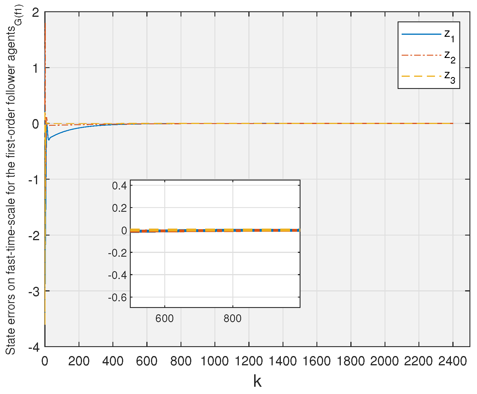
In order to clearly and intuitively observe the change of the state observation error of each follower agent in the whole MAS, the sum of the absolute value of the observation error of each dimensional state variable of each follower agent on the slow-time scale and the fast-time scale is considered (that is, the 1-norm of the state observation errors of each follower agent). Moreover, its change trajectory along with k is shown in Figure 7 and Figure 8. As can be seen from the figures, the state errors of the whole MAS converge to zero.

Finally, the initial states, final states and trajectories of all followers are shown in Figure 9. First-order and second-order agents are marked with circles and asterisks, respectively.

7. Conclusions

This paper presents and investigates for the first time the observability of discrete-time two-time-scale MASs with heterogeneous features under leader-based architecture, which complements the existing results on the observability of MASs. During the study, this class of MASs was first modeled based on the theory of singularly perturbed systems and then reduced to a slow-time-scale subsystem and a fast-time-scale subsystem based on the boundary layer method of singularly perturbed systems, avoiding the possible numerical ill-posedness problem when the systems are directly analyzed by classical methods. Then, some more practical and operational criteria were obtained in conjunction with matrix theory. Finally, an example was given whose simulation results verified the validity of the conclusions. The next step of the work will consider the observability of MASs with multiple time scales.

References

1. Wang, X.; Wang, X.; Su, H.; Lam, J. Reduced-order interval observer based consensus for MASs with time-varying interval uncertainties. Automatica 2022, 135, 109989. [Google Scholar] [CrossRef]
2. Wang, X.; Su, H.; Zhang, F.; Zemouche, A.; Chen, G. Interval observer design and consensus of multiagent systems with time-varying interval uncertainties. SIAM J. Control Optim. 2021, 59, 3392–3417. [Google Scholar] [CrossRef]
3. Lu, X.; Li, H. An improved stability theorem for nonlinear systems on time scales with application to multi-agent systems. IEEE Trans. Circuits Syst. II Express Briefs 2020, 67, 3277–3281. [Google Scholar] [CrossRef]
4. Gu, M.; Jiang, G.P.; Qian, J.; Wu, Y. Group controllability of discrete-time second-order multi-agent systems with two-time-scale feature. Asian J. Control 2022, 24, 755–770. [Google Scholar] [CrossRef]
5. Wang, X.; Su, H.; Zhang, F.; Chen, G. A robust distributed interval observer for LTI systems. IEEE Trans. Autom. Control 2022. [Google Scholar] [CrossRef]
6. Ning, B.; Han, Q.L.; Ding, L. Distributed finite-time secondary frequency and voltage control for islanded microgrids with communication delays and switching topologies. IEEE Trans. Cybern. 2020, 51, 3988–3999. [Google Scholar] [CrossRef]
7. Tanner, H.G. On the controllability of nearest neighbor interconnections. In Proceedings of the 2004 43rd IEEE Conference on Decision and Control (CDC) (IEEE Cat. No. 04CH37601), Nassau, Bahamas, 14–17 December 2004; IEEE: Piscataway, NJ, USA, 2004; Volume 3, pp. 2467–2472. [Google Scholar]
8. Sundaram, S.; Hadjicostis, C.N. Structural controllability and observability of linear systems over finite fields with applications to multi-agent systems. IEEE Trans. Autom. Control 2012, 58, 60–73. [Google Scholar] [CrossRef]
9. Liu, Y.Y.; Slotine, J.J.; Barabási, A.L. Observability of complex systems. Proc. Natl. Acad. Sci. USA 2013, 110, 2460–2465. [Google Scholar] [CrossRef]
10. Lozano, R.; Spong, M.W.; Guerrero, J.A.; Chopra, N. Controllability and observability of leader-based multi-agent systems. In Proceedings of the 2008 47th IEEE Conference on Decision and Control, Cancun, Mexico, 9–11 December 2008; IEEE: Piscataway, NJ, USA, 2008; pp. 3713–3718. [Google Scholar]
11. Sabattini, L. Controllability and Observability Preservation for Networked Systems with Time Varying Topologies. IFAC Proc. Vol. 2014. [Google Scholar] [CrossRef]
12. Liu, B.; Xu, N.; Su, H.; Wu, L.; Bai, J. On the observability of leader-based multiagent systems with fixed topology. Complexity 2019, 2019, 1–10. [Google Scholar] [CrossRef]
13. Tian, L.; Guan, Y.; Wang, L. Controllability and observability of switched multi-agent systems. Int. J. Control 2019, 92, 1742–1752. [Google Scholar] [CrossRef]
14. Zelazo, D.; Mesbahi, M. On the observability properties of homogeneous and heterogeneous networked dynamic systems. In Proceedings of the 2008 47th IEEE Conference on Decision and Control, Cancun, Mexico, 9–11 December 2008; IEEE: Piscataway, NJ, USA, 2008; pp. 2997–3002. [Google Scholar]
15. Tian, L.; Guan, Y.; Wang, L. Controllability and observability of multi-agent systems with heterogeneous and switching topologies. Int. J. Control 2020, 93, 437–448. [Google Scholar] [CrossRef]
16. Dwivedy, S.K.; Eberhard, P. Dynamic analysis of flexible manipulators, a literature review. Mech. Mach. Theory 2006, 41, 749–777. [Google Scholar] [CrossRef]
17. Pósfai, M.; Gao, J.; Cornelius, S.P.; Barabási, A.L.; D’Souza, R.M. Controllability of multiplex, multi-time-scale networks. Phys. Rev. E 2016, 94, 032316. [Google Scholar] [CrossRef] [PubMed]
18. Long, M.; Su, H.; Liu, B. Group controllability of two-time-scale multi-agent networks. J. Frankl. Inst. 2018, 355, 6045–6061. [Google Scholar] [CrossRef]
19. Long, M.; Su, H.; Liu, B. Second-order controllability of two-time-scale multi-agent systems. Appl. Math. Comput. 2019, 343, 299–313. [Google Scholar] [CrossRef]
20. Long, M.; Su, H.; Liu, B. Second-order controllability of two-time-Scale discrete-time multi-agent systems. IET Control Theory Appl. 2019, 13, 2356–2364. [Google Scholar] [CrossRef]
21. Su, H.; Long, M.; Zeng, Z. Controllability of two-time-scale discrete-time multiagent systems. IEEE Trans. Cybern. 2018, 50, 1440–1449. [Google Scholar] [CrossRef]
22. Long, M.; Su, H.; Wang, X.; Liu, B. Controllability of heterogeneous multiagent systems with two-time-scale feature. Chaos Interdiscip. J. Nonlinear Sci. 2019, 29, 043116. [Google Scholar] [CrossRef]
23. Kokotović, P.; Khalil, H.K.; O’reilly, J. Singular Perturbation Methods in Control: Analysis and Design; SIAM: Philadelphia, PA, USA, 1999. [Google Scholar]
24. Boyd, S.; El Ghaoui, L.; Feron, E.; Balakrishnan, V. Linear Matrix Inequalities in System and Control Theory; SIAM: Philadelphia, PA, USA, 1994. [Google Scholar]
25. Chow, J.; Kokotovic, P. A decomposition of near-optimum regulators for systems with slow and fast modes. IEEE Trans. Autom. Control 1976, 21, 701–705. [Google Scholar] [CrossRef]
26. Mahmoud, M.S. Design of observer-based controllers for a class of discrete systems. Automatica 1982, 18, 323–328. [Google Scholar] [CrossRef]
27. Litkouhi, B.; Khalil, H. Multirate and composite control of two-time-scale discrete-time systems. IEEE Trans. Autom. Control 1985, 30, 645–651. [Google Scholar] [CrossRef]
28. Kokotovic, P. A Riccati equation for block-diagonalization of ill-conditioned systems. IEEE Trans. Autom. Control 1975, 20, 812–814. [Google Scholar] [CrossRef]
29. Kalman, R.E.; Bertram, J.E. Control system analysis and design via the “second method” of Lyapunov: I—Continuous-time systems. J. Basic Eng. 1960, 82, 371–393. [Google Scholar] [CrossRef]
Figure 1. Legend for a discrete-time MAS with heterogeneous and two-time-scale features in the leader–follower architecture.
Mathematics 11 01907 g001
Figure 2. A MAS composed of nine agents.
Mathematics 11 01907 g002
Figure 3. State errors on slow-time-scale for the first-order follower agents.
Mathematics 11 01907 g003
Figure 4. State errors on slow-time scale for the second-order follower agents.
Mathematics 11 01907 g004
Figure 5. State errors on fast-time scale for the first-order follower agents.
Mathematics 11 01907 g005
Figure 6. State errors on fast-time scale for the second-order follower agents.
Mathematics 11 01907 g006
Figure 7. The 1-norm of the state observation errors of all the follower agents on slow-time scale.
Mathematics 11 01907 g007
Figure 8. The 1-norm of the state observation errors of all the follower agents on fast-time scale.
Mathematics 11 01907 g008
Figure 9. Trajectories of all follower agents.
Mathematics 11 01907 g009
Disclaimer/Publisher’s Note: The statements, opinions and data contained in all publications are solely those of the individual author(s) and contributor(s) and not of MDPI and/or the editor(s). MDPI and/or the editor(s) disclaim responsibility for any injury to people or property resulting from any ideas, methods, instructions or products referred to in the content.