ICMFed: An Incremental and Cost-Efficient Mechanism of Federated Meta-Learning for Driver Distraction Detection

Abstract

Driver distraction detection (3D) is essential in improving the efficiency and safety of transportation systems. Considering the requirements for user privacy and the phenomenon of data growth in real-world scenarios, existing methods are insufficient to address four emerging challenges, i.e., data accumulation, communication optimization, data heterogeneity, and device heterogeneity. This paper presents an incremental and cost-efficient mechanism based on federated meta-learning, called ICMFed, to support the tasks of 3D by addressing the four challenges. In particular, it designs a temporal factor associated with local training batches to stabilize the local model training, introduces gradient filters of each model layer to optimize the client–server interaction, implements a normalized weight vector to enhance the global model aggregation process, and supports rapid personalization for each user by adapting the learned global meta-model. According to the evaluation made based on the standard dataset, ICMFed can outperform three baselines in training two common models (i.e., DenseNet and EfficientNet) with average accuracy improved by about 141.42%, training time saved by about 54.80%, communication cost reduced by about 54.94%, and service quality improved by about 96.86%.

1. Introduction

Currently, even though vehicles are upgraded to support a higher level of autonomy, humans are still their primary operators. Therefore, driver distraction is still a major problem that can disrupt and jeopardize transportation systems [1,2]. In general, driver distraction occurs when a driver’s attention is diverted, leading to a delay in recognizing vital information to keep vehicles running safely [3]. Especially with the proliferation of in-vehicle multimedia devices and personal smart gadgets, diverse in-vehicle activities exacerbate driver distraction. To prevent potential hazards and incidents, warnings to distracted drivers need to be fast and precise, which shows the necessity of driver distraction detection (3D).

With the rapid development of advanced technologies, e.g., Artificial Intelligence and Internet of Things (IoT), the capabilities of in-vehicle devices have improved, such as sensing, communication, computing, etc. Intelligent vehicle systems are often equipped with rich computing capabilities to support various tasks. Particularly, data-driven approaches to deep learning models have been widely developed and applied to support 3D, e.g., with various core models that are trained on driver face poses [4], driving actions [5], electroencephalography signals [6], and other sensed information to detect distractions, such as unfocused eyesight [7], inattention [6], and inappropriate operation [5].

Traditional deep learning methods centrally process data, namely, vehicles need to upload signals, images, and other sensed data to a central server. After the collection of sensed data, the server will train the required model based on the data consolidated from multiple sensing devices, also known as smart vehicles. However, in this process, the data to be transmitted may contain private or sensitive information, such as travel trajectories and passenger profiles. It is vulnerable to being intercepted and attacked via network connections between vehicles and servers. Under the restrictions listed in recently announced data protection laws and regulations, more isolated data silos are formed and become unbreakable barriers to applying centralized model learning solutions [8]. Therefore, federated learning (FL) is emerging as a feasible solution that can train models without private and sensitive information leaving its local repository [8,9].

Even though various solutions are proposed by using FL to upgrade the model learning paradigm of 3D [10,11,12], they are still incapable of handling the dynamics and heterogeneity encountered in the daily usage of 3D. First, most recent research is conducted based on predefined experimental settings, in which clients possess preassigned data and exchange model parameters directly without any optimizations. Specifically, in more realistic scenarios, data can be sensed continuously. Since current solutions focus more on old data, if they are applied to the incremental data directly, it may make the model learning inefficient, leading to catastrophic forgetting of knowledge [13]. Second, even though current solutions based on FL do not need to transmit raw data, it is still costly to train high-performance models based on more frequent and excessive client–server interactions [9]. Finally, it is common to see that the availability of local data and computing powers of moving vehicles may change over time and place, and this may make current solutions inefficient at not only accommodating heterogeneous devices but also data with various distributions, uneven sizes, and missing label classes [9,14,15].

To tackle the aforementioned challenges, this paper proposes an incremental and cost-efficient mechanism for federated meta-learning, named ICMFed, to support 3D. In general, ICMFed integrates incremental learning and meta-learning with federated learning to provide a novel learning paradigm that can be applied to address the dynamics and heterogeneity within real-world 3D scenarios. The main contributions of this work can be summarized as follows:

• ICMFed introduces temporal factors on batches created according to sample sensed time ascendingly, which can ensure rapid and balanced extraction of features from gradually accumulated data. Meanwhile, by calculating the gradient similarity of model layers, a layer-wise model uploading process is implemented to reduce communication costs without degrading the model performance.
• Taking advantage of meta-learning and federated learning, ICMFed can remedy the impact of heterogeneity in data and devices to learn the global meta-model by employing a weighted model aggregation strategy, which enhances the model aggregation process by an adaptive weight calculated based on the richness of local information.
• Through the evaluation based on the 3D dataset collected by State Farm and two classical models, ICMFed can not only significantly elevate the learning performance, i.e., communication cost and learning accuracy, but also dramatically improve related service quality.

The remainder of this paper is organized as follows. Section 2 summarizes related challenges and solutions. Then, ICMFed is presented and evaluated in Section 3 and Section 4, respectively. Finally, Section 5 concludes this work and presents future research directions.

2. Challenges and Related Work

This section first introduces four challenges regarding the dynamics and heterogeneity encountered in incremental federated meta-learning (IFM), and accordingly, related solutions are discussed.

2.1. Emerging Challenges

First, as for the dynamics in real-world scenarios, the following two critical challenges are faced by 3D:

• C1.1 Data Accumulation. While the 3D service is installed, the vehicles can continuously sense driver status and increase the samples to be used for model updates. In comparison to static scenarios where the training samples will not change frequently, data accumulation can cause pre-trained knowledge to be obsolete in processing new data [13,16].
• C1.2 Communication Optimization. To train a model jointly, 3D services require frequent interaction between the clients and the server. Even though in IFM, model parameters are exchanged instead of entire data, which can reduce the network traffic [8], the client–server interaction frequency increases to update the model iteratively, resulting in high latency to update the model on the fly [9,17,18].

Moreover, the heterogeneity embedded in 3D is represented by two main aspects, namely:

• C2.1 Data Heterogeneity. Due to the restriction in IFM, data sensed are stored locally to protect user privacy, and as a result, the local data of different users may vary to be non-iid (non-independent and identically distributed), i.e., different distribution of samples, uneven data quality, etc. Such heterogeneity can significantly complicate the learning process of IFM [15,18].
• C2.2 Device Heterogeneity. The devices to support 3D may have different configurations in terms of software and hardware, e.g., operation systems, sensing capabilities, storage spaces, computing powers, etc. Moreover, on the device, more than one service is running in parallel, and as a result, the availability of learning resources may vary among them. Therefore, how to select proper clients becomes an emerging challenge in IFM to remedy the impact of such heterogeneity [19,20,21].

2.2. Related Solutions

To tackle the abovementioned challenges, related solutions are proposed.

2.2.1. Solutions to Data Accumulation

The data accumulation of IFM can be solved by timely updating of global models or optimizing local training patterns. While considering incremental scenarios, if the global model or training task is not updated adequately and in a timely manner, it will lead to poor performance [22,23]. Current research commonly adopts a predefined configuration for model learning [8,15,24]. Moreover, without modifying the model structure, several methods optimize local training patterns to improve knowledge retention on both old and new samples. For example, Wei et al. [22] proposed a method named FedKL utilizing knowledge lock to maintain the previously learned knowledge. Yoon et al. [25] introduced FedWeIT, allowing clients to leverage indirect experience from other clients to support continuous learning of federated knowledge. Le et al. [26] suggested a weighted processing strategy for model updating to prevent catastrophic forgetting. However, to achieve the optimal performance of these methods, the training will become less efficient, especially to process non-iid data.

2.2.2. Solutions to Communication Optimization

There are two major approaches for communication optimization, i.e., minimizing the amount of data exchanges or reducing the size of data transmitted. Specifically, the first approach can be achieved by reducing model upload frequency [27,28], adjusting aggregation schedules [28,29,30], and optimizing network topology [9,31]. In addition, technologies such as knowledge distillation [10,24] and sparse compression [25,32] can be used to compress parameters exchanged without degrading model performance. Finally, the significance of each model layer can be determined in order to perform layer-wise uploading based on user similarity [33], model similarity [34,35], etc.

2.2.3. Solutions to Data Heterogeneity

Data heterogeneity, in general, can be addressed by knowledge distillation or meta-learning. Specifically, as for knowledge distillation, Lin et al. [24] proposed a FedDF framework, combining federated learning with knowledge distillation. Shang et al. [10] presented FedBiKD, which is a simple and effective federated bidirectional knowledge distillation framework. Moreover, meta-learning as the process of learning how to learn can guide local learning for better performance. There are many meta-learning algorithms, e.g., Model-Agnostic Meta-learning (MAML) [36], First-Order Model-Agnostic Meta-learning (FOMAML) [37], and Reptile [38]. The joint utilization of meta-learning algorithms and federated learning enables quick, personalized, and heterogeneity-supporting training [14,15,39]. Federated meta-learning (FM) offers various similar applications in transportation to overcome data heterogeneity, such as parking occupancy prediction [40,41] and bike volume prediction [42].

2.2.4. Solutions to Device Heterogeneity

In general, client heterogeneity can be resolved by client selection prior to task start and weighting during global aggregation. To simplify the learning process, random or full client selection is commonly utilized [8,26,34], under the prerequisite that all clients need to be available with little performance disparity. Thus, more advanced strategies are designed to mitigate the unreliability among clients, e.g., a compensatory first-come-first-merge algorithm adopted by Wu et al. [43], and the dynamic selection based on the status and availability of clients considered by Huang et al. [44]. Moreover, aggregation weights are also widely discussed. Particularly, the size of local samples [8,31,34] is the most common weight, but with drawbacks to handling IFM as the size of samples can change over time and place. Hence, weights relevant to the characteristics of devices are introduced, such as information richness [30], temporal weight [28,30], etc.

In summary, as summarized in Table 1, existing methods focus more on solving the optimization issues related to communication (i.e., C1.2), and also present visible progress in addressing the two challenges in heterogeneity (i.e., C2.1 and C2.2). However, it is still missing a solution that can resolve the four challenges encountered in IFM. Therefore, ICMFed is proposed with dedicatedly designed model learning and adaptation processes to not only boost the learning performance but also improve the service quality.

Table 1. The overview of related works (○ NOT SUPPORTED and ● SUPPORTED).

Related Work	C1.1	C1.2	C2.1	C2.2
FedAVG [8]	○	●	●	○
FedBiKD [10]	○	●	●	○
Per-FedAvg [14]	○	○	●	○
FedMeta [15]	○	○	●	○
FedKL [22]	○	○	●	○
FedDF [24]	●	●	○	○
FedWeIT [25]	●	○	●	○
FCL-BL [26]	●	●	○	○
Fed2a [28]	○	●	○	●
ASO-Fed [29]	○	●	●	○
TrisaFed [30]	○	●	○	●
HFL [31]	○	●	○	●
STC [32]	○	●	●	○
COFEL [34]	○	●	○	●
FedReptile [39]	○	○	●	○
SAFA [43]	○	●	○	●
RBCS-F [44]	○	●	○	●
This paper (ICMFed)	●	●	●	●

3. Methodology

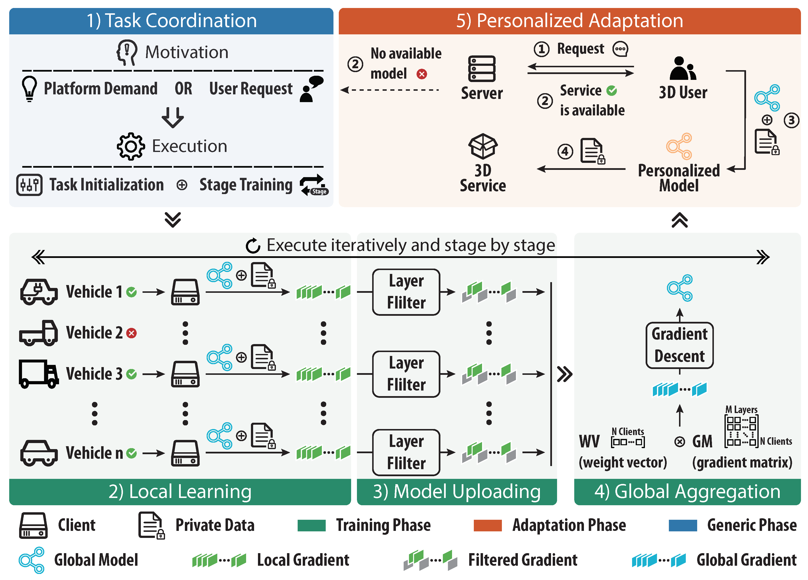
To tackle the challenges mentioned above, an incremental and cost-efficient mechanism of federated meta-learning called ICMFed is proposed. As illustrated in Figure 1, essentially, it comprises five consecutive stages, i.e., (1) Task Coordination: The server will start the task on demand and perform stage transition periodically in incremental scenarios; (2) Local learning: The participant vehicles, i.e., clients, will execute local meta-training based on their own data accumulated continuously; (3) Model uploading: Each client calculates and filters the gradients of layers of the updated local model, and then uploads them to the server dynamically; (4) Global aggregation: The server receives and aggregates the local model gradients to update the global model; (5) Personalized adaptation: Based on the trained global meta-knowledge, user vehicles can execute few rounds of local training to gain their personalized models. Additionally, stages 2–4 belong to the training phase, stage 5 is the adaptation phase, and stage 1 is the generic phase supporting both the training and adaptation phases.

Figure 1. The overall workflow of ICMFed. Specifically, stage 1 is the generic phase supporting both training and adaptation phases; stages 2 to 4 belong to the training phase, executing training iteratively and stage by stage; and stage 5 is the adaptation phase to quickly train personalized models for the clients.

In this section, we first define the problem and then describe in detail the five stages of ICMFed. In addition, the key notations and their explanations appearing below are summarized in Table 2.

Table 2. Notations and explanations.

Module	Notation	Description
Client	C	The client set. A client can be represented by c, $c\in C$
	$C_s$	The client set for training in a stage s.
	$C_e$	The client set for evaluation.
	u	The target user, who requires 3D services.
Coefficient	$CI{R}_{c,s}$	Client information richness, e.g., calculated by information entropy.
	$cs{l}_{c,s}^{r,l}$	Cosine similarity of layer l in learning round r, whose values range from $[-1,1]$.
	$CS{V}_{c,s}^r$	Cosine similarity vector composed by $cs{l}_{c,s}^{r,l}$, whose size is $1\times L$.
	$G{M}_s^r$	Gradient matrix composed by $g_{c,s}^{r,l}$, whose size is $\left|C\right|\times L$.
	$SI{P}_{c,s}$	Stage incremental proportion of clients.
	$w_{c,s}$	Aggregation weight calculated based on $SI{P}_{c,s}$ and $CI{R}_{c,s}$.
	$W{V}_s$	Weight vector composed by $w_{c,s}$, whose size is $1\times \left|C\right|$.
Data	B	Number of batches split for training. Each batch can also be represented by b.
	$D_c$	Data of client c, generally consisting of feature $X_c$ and label $Y_c$.
	$D_{c,s}$	Data at the initial stage.
	$D_{c,s:s+1}$	Incremental data between two adjacent stages.
	$D_{c,s}^{spt}$	Support set for FM.
	$D_{c,s}^{qry}$	Query set for FM.
Function	$\mathcal{L}(\theta ,D)$	Loss function based on model parameters $\theta$ and the data D.
	$N\left(x\right)$	Simplified representation of the normalization function.
	$sum\left(X\right)$	Function to sum the elements in matrix X.
Hyperparameter	$\alpha$	Local learning rate, also called inner learning rate.
	$\beta$	Global learning rate, also called outer learning rate.
	$\gamma$	Adaptation learning rate for target users.
	$\mu$	The threshold for layer filter.
	R	Total number of rounds within a stage. Each round can also be represented by r.
	S	Total number of stages. Each stage can also be represented by s.
Model	${\theta }_{c,s}^r$	Local model parameter.
	${\widehat{\theta }}_{c,s}^r$	Intermediate model parameter.
	${\theta }_{glo,s}^r$	Global model parameter.
	$g_{c,s}^r$	Gradient of local model. Each layer of it can also be represented by $g_{c,s}^{r,l}$.
	$g_{glo,s}^r$	Gradient of global model. Each layer of it can also be represented by $g_{glo,s}^{r,l}$.
	L	Layer number of the model. A individual layer is marked as l, $l\in L$.

3.1. Problem Definition

For typical FL tasks, the basic framework typically consists of a server and client set C. Each client $c\in C$ will perform local learning using private data, denoted as $D_c=\{X_c,Y_c\}$. Especially in FM, $D_c$ will be further split into a support set $D_c^{spt}$ and a query set $D_c^{qry}$. Based on the support and query sets, FM aims to find a model initialization (i.e., meta-knowledge) that can perform well on heterogeneous clients to be quickly adapted with the local gradient descent defined in Formula (1).

$$\begin{array}{c}{\displaystyle \underset{\theta \in {\mathbb{R}}^d}{min}}\frac{1}{\left|C\right|}{\displaystyle \sum _{c\in C}}{\mathcal{L}}_c(\theta -\alpha ▿{\mathcal{L}}_c(\theta ,D_c^{spt}),D_c^{qry})\end{array}$$

(1)

where $\theta \in {\mathbb{R}}^d$ are the model parameters; $\alpha$ stands for the local learning rate, also commonly called inner learning rate; and ${\mathcal{L}}_c$ represents the loss function of client c (by default, cross-entropy for 3D).

In the case of real-world applications of FM as in 3D, both the number of available clients and the size of local data may change dynamically, i.e., online statuses of participant vehicles and driver conditions sensed by in-vehicle devices may vary over time and place. Therefore, we divide the learning task into multiple stages, since the pre-trained knowledge in incremental scenarios may become invalid as it may drift while new data are sensed.

Therefore, the timing of stage transitions shall be determined, which is based on the number of training rounds in this work. The training objects within a stage s are as static as FM, i.e., the client set for training $C_s$ is fixed and takes data at initialization of stage $D_s$ as training samples. When discussing the transition to a new stage $s+1$, new clients are selected as $C_{s+1}$ while the incremental data $D_{s:s+1}$ are updated according to Formula (2).

$$\begin{array}{c}{D}_{s+1}=D_s\cap D_{s:s+1}\end{array}$$

(2)

In general, as indicated by Formula (3), the goal of IFM is to maintain high model performance in each stage. Accordingly, ICMFed is designed to minimize the usage of communication resources and reduce the time consumption of model training through the five stages, i.e., task coordination, local learning, model uploading, global aggregation, and personalized adaptation.

$$\begin{array}{c}{\displaystyle \underset{{\theta }_s\in {\mathbb{R}}^d}{min}}\frac{1}{|C_s|}{\displaystyle \sum _{c\in C_s}}{\mathcal{L}}_c({\theta }_s-\alpha ▿{\mathcal{L}}_c({\theta }_S,D_{c,s}^{spt}),D_{c,s}^{qry})\end{array}$$

(3)

3.2. Task Coordination

The main tasks of the server are to (1) start the learning tasks according to the actual needs, and (2) coordinate learning participants for the meta-knowledge. In general, the initialization of learning tasks is triggered by the server, when the performance of the deployed model decreases significantly, or users with limited local data in the learning consortium require a model to assist the 3D task. Moreover, the server is also responsible for the management of clients and the transition of stages. Note that when a task begins, the server will first select adequate clients as learning participants and then dispatch training-related information (such as the current global model, predefined hyperparameters, etc.) to them.

3.3. Local Learning

In each client, ICMFed conducts the local training through four steps, i.e., (1) training initialization, (2) data sampling, (3) model training, and (4) gradient calculation, which are described below.

3.3.1. Step 1: Training Initialization

Since the mechanism is targeted synchronously, each client will receive the most recent global model parameters ${\theta }_{glo}$ from the server at the beginning of each learning round. The initial model parameters of client c in round r of stage s can be represented by Formula (4).

$$\begin{array}{c}{\theta }_{c,s}^r={\theta }_{glo,s}^{r-1}\end{array}$$

(4)

where ${\theta }_{glo,s}^0$ is the initialized global model parameters of stage s.

3.3.2. Step 2: Data Sampling

Within a client c, the local data are sampled into a support set $D_{c,s}^{spt}$ and a query set $D_{c,s}^{qry}$. Then, $D_{c,s}^{spt}$ will again be split into B batches with their samples ordered ascendingly according to the created time. The main purpose of batch splitting is to maintain the temporal information in the model-updating step as described below.

3.3.3. Step 3: Model Updating

After the preparation of training samples, the client will update its local model parameters based on the support set, as shown in Formula (5).

$$\begin{array}{c}{\widehat{\theta }}_{c,s}^r={\theta }_{c,s}^r-\alpha {\displaystyle \sum _{b\in [1,B]}}{e}^{-\frac{b}{B}}{▿}_{{\theta }_{c,s}^{r,b-1}}{\mathcal{L}}_c({\theta }_{c,s}^{r,b-1},D_{c,s}^{spt,b})\end{array}$$

(5)

where ${\widehat{\theta }}_{c,s}^r$ is the intermediate model parameter; b stands for batch id; $D_{c,s}^{spt,b}$ represents the $b^{th}$ batch of $D_{c,s}^{spt}$; and $e^{-\frac{b}{B}}$ is named as timing factor to adjust the step size of gradient descent according to the temporal information of each batch.

Local models in ICMFed conduct multiple batch gradient descent inside a round, whereas the general local training of FM processes the dataset to generate one gradient descent for the model parameter learning. Moreover, ICMFed employs the optimization on the temporal batches based on the timing factors, to ensure that the model feature extraction process can be quickly adapted among clients to simplify and unify the model learning behavior.

3.3.4. Step 4: Gradient Calculation

ICMFed can support FOMAML or Reptile to calculate the gradient required in updating the global meta-model. In general, besides the gradient calculated based on the support set as in Reptile, FOMAML also needs the gradient from the query set. The two modes are expressed in Formula (6) (FOMAML) and Formula (7) (Reptile), respectively.

$$\begin{array}{c}{g}_{c,s}^r={▿}_{{\widehat{\theta }}_{c,s}^r}\mathcal{L}({\widehat{\theta }}_{c,s}^r,D_{c,s}^{qry,b})\end{array}$$

(6)

$$\begin{array}{c}{g}_{c,s}^r={\widehat{\theta }}_{c,s}^r-{\theta }_{glo,s}^{r-1}\end{array}$$

(7)

where $g_{c,s}^r$ is the uploaded gradient of client c in round r of stage s.

3.4. Model Uploading

After obtaining the uploaded gradients, clients need to upload the gradients to the server via the network. Note that as the number of clients grows or the model structure becomes more complicated, uploading multi-layer parameters will incur large communication costs. Therefore, an adaptive filter is proposed to upload valuable and critical layers without jeopardizing the overall model performance.

Accordingly, ICMFed applies the cosine similarity vector (CSV) as the measure of the layer filter [45,46]. CSV, expressed by Formula (8), calculates the directional correlation of each layer between the local and global parameters in the adjacent round.

$$\begin{array}{c}CS{V}_{c,s}^r={\left. [\begin{array}{cccc}cs{l}_{c,s}^{r,1}& cs{l}_{c,s}^{r,2}& \cdots & cs{l}_{c,s}^{r,L}\end{array}\right]}_{1\times L}\end{array}$$

(8)

where L is the number of model layers, which is a constant value in a task; $cs{l}_{c,s}^{r,l}\in [-1,1]$ is the cosine similarity of layer l, which can be expressed by Formula (9).

$$\begin{array}{c}cs{l}_{c,s}^{r,l}=\frac{sum(g_{c,s}^{r,l} \circ g_{glo,s}^{r,l})}{\sqrt{sum(g_{c,s}^{r,l} \circ g_{c,s}^{r,l})} \times \sqrt{sum(g_{glo,s}^{r,l} \circ g_{glo,s}^{r,l})}}\end{array}$$

(9)

where ∘ is the Hadamard Product; and $sum\left(X\right)$ is a function to sum the elements in matrix X. Based on hyperparameter $\mu$ designed as a threshold for the layer filter, client c will not upload the parameter of layer l when $cs{l}_{c,s}^{r,l}\ge \mu$.

However, while the global model is already distributed in the form of model parameters, broadcasting the global parameters to clients every round would significantly increase communication costs. To reduce such cost, the global gradient can be obtained from continuous alterations in global models, as shown in Formula (10).

$$\begin{array}{c}{g}_{glo,s}^{r,l}\approx -({\theta }_{glo,s}^r-{\theta }_{glo,s}^{r-1})\end{array}$$

(10)

where ${\theta }_{glo,s}^0={\theta }_{glo,s-1}^R$, i.e., the parameters in the last round of the previous stage, where R is the total learning rounds per stage. Note that no layer filtering is required in the first round of the first stage.

Following the layer filter, clients can upload parameters via the network, e.g., wireless communication with roadside devices.

3.5. Global Aggregation

After the receipt of local updates from the clients, the global aggregation is executed in the server in three steps, e.g., parameter collation, weight analysis, and model updating.

3.5.1. Step 1: Parameter Collation

The server will continuously receive the gradient parameters submitted by clients. In synchronous mode, the server will wait for all clients to upload parameters and then use the formed gradient matrix (GM, as defined in Formula (11)) for the aggregation.

$$\begin{array}{c}G{M}_s^r={\left. [\begin{array}{cccc}{g}_{1,s}^{r,1}& g_{1,s}^{r,2}& \cdots & g_{1,s}^{r,L}\\ g_{2,s}^{r,1}& g_{2,s}^{r,2}& \cdots & g_{2,s}^{r,L}\\ ⋮& ⋮& \ddots & ⋮\\ g_{C,s}^{r,1}& g_{C,s}^{r,2}& \cdots & g_{C,s}^{r,L}\end{array}\right]}_{\left|C\right|\times L}\end{array}$$

(11)

Note that if $g_{c,s}^{r,l}$ is not successfully received in a predefined amount of waiting time, i.e., the value is null, it would be substituted by the corresponding layer of the previous global gradient, as indicated in Formula (12).

$$\begin{array}{c}{g}_{c,s}^{r,l}=\left\{\begin{array}{cc}{g}_{c,s}^{r,l},\hfill & g_{c,s}^{r,l}\ne None\hfill \\ g_{glo,s}^{r-1,l},\hfill & g_{c,s}^{r,l}=None\hfill \end{array}\right.\end{array}$$

(12)

3.5.2. Step 2: Weight Analysis

Existing FM mechanisms tend to aggregate $GM$ directly to update the global model, but this is not suitable in IFM scenarios. As in incremental scenarios, the data heterogeneity of clients is amplified, and treating them equally will impact the overall model performance.

To tackle it, ICMFed designs a weight vector (WV) based on stage incremental proportion (SIP) and client information richness (CIR). Specifically, SIP indicates the proportion of newly sensed data in a stage, as shown in Formula (13). CIR is the information entropy of the training data. WV can be quantified in three ways, i.e., SIP, CIR, and a mixture of the two, as given by Formula (14).

$$\begin{array}{c}SI{P}_{c,s}=\frac{|D_{c,s-1:s}|}{|D_{c,s}|}\end{array}$$

(13)

$$\begin{array}{c}W{V}_s={\left. [\begin{array}{cccc}{w}_{1,s}& w_{2,s}& \cdots & w_{C,s}\end{array}\right]}_{1\times \left|C\right|}\\ s.t.w_{c,s}=\{N\left(SI{P}_{c,s}\right),N\left(CI{R}_{c,s}\right),N(SI{P}_{c,s},CI{R}_{c,s})\}\end{array}$$

(14)

where $N\left(x\right)$ is a normalization function, i.e., Softmax.

3.5.3. Step 3: Model Updating

Finally, global gradient and updated global model parameters in round r of stage s can be obtained according to Formula (15) and Formula (16), respectively.

$$\begin{array}{c}{g}_{glo,s}^r=W{V}_s\times G{M}_s^r\end{array}$$

(15)

$$\begin{array}{c}{\theta }_{glo,s}^r={\theta }_{glo,s}^{r-1}-\beta g_{glo,s}^r\end{array}$$

(16)

where $\beta$ stands for the global learning rate.

After the model updating, related training content will be distributed to the clients. The training contents include training configurations, updated model parameters, and flags to harmonize tasks.

3.6. Personalized Adaptation

Users who use 3D services can download the current global meta-model to train personalized models based on their local data as illustrated in Formula (17).

$$\begin{array}{c}{\theta }_u={\theta }_{glo}-\gamma {▿}_{{\theta }_{glo}}\mathcal{L}({\theta }_{glo},D_u)\end{array}$$

(17)

where u represents the target user; and $\gamma$ is the adaptation learning rate, which is recommended to be equal to $\alpha$. With one or a few epochs of gradient descent, a personalized model can be learned and applied.

3.7. Algorithm of ICMFed

Besides the preparation of the learning in phase 1 of ICMFed, the training and adaptation phases present the main workflow of ICMFed in each stage. The algorithms of these two phases are described below, respectively.

3.7.1. Algorithm of Training Phase

As listed in Algorithm 1, this phase consists of two parts, namely:

Algorithm 1 Training phase of ICMFed

PART 1:  Pseudocode for the server. 1: Initialize and start a task; 2: for stage $s\in [1,S]$ do 3:       Select clients and send the “SELECTED” signal; 4:       Distribute the training configuration, e.g., model structure, hyperparameters, etc.; 5:       for round $r\in [1,R]$ do 6:             Distribute current global model parameters ${\theta }_{glo,s}^{r-1}$ to the selected clients; 7:             Send “TRAIN” signal to the selected clients; 8:             Wait for local parameters from the selected clients; 9:             Receive local model gradient $g_{c,s}^r$ from each selected client; 10:           Calculate aggregation weight $w_{c,s}$; 11:           Update global model parameters ${\theta }_{glo,s}^r$ according to Formula (16); 12:     end for 13:     if Task termination conditions are met then 14:           Send “STOP” signal and distribute the latest global model to all clients; 15:     else 16:           Transit to the next stage; 17:     end if 18: end for PART 2:  Pseudocode for the client; 19: if “SELECTED” signal is received then 20:       Prepare itself according to the training configurations; 21:       Sample a support set $D_{c,s}^{spt}$ with B batches and a query set $D_{c,s}^{qry}$; 22:       Initialize local model according to Formula (4); 23: else if “TRAIN” signal is received then 24:       Update local model according to Formula (5); 25:       Calculate gradient according to Formula (6) or Formula (7); 26:       Upload local gradient and the required parameters to calculate aggregation weight; 27: else if “STOP” signal is received then 28:       Stop local training; 29: end if

1.

Part 1 at the server. After the initialization of the task, the server will iteratively and periodically perform model training according to the settings. First, the server will choose qualified clients at the beginning of each learning round. Note that the server will perform model aggregation only after all selected clients upload their parameters or the predefined waiting time is exceeded. The termination conditions will be determined once a single training stage is completed. Particularly, the conditions can be the performance target, task execution time, etc.

2.

Part 2 at each client. The clients will take various actions based on the signals received from the server. When a client is selected to perform a training stage, it will sample the training dataset and initialize the local model training. In each training round, clients update and upload their local model after the receipt of the global meta-model parameters from the server. Clients perform their learning tasks through continuous interactions with the server.

3.7.2. Algorithm of Adaptation Phase

As indicated in Algorithm 2, this phase also consists of two parts. The server periodically makes the recently trained global meta-model available to be downloadable by users who require 3D capabilities (also known as the target users). Accordingly, the target clients can download available models on demand. Due to the advantages of FM, the model to support 3D services can benefit from the fast adaptation of meta-knowledge to be personalized.

Algorithm 2 Adaptation phase of ICMFed

PART 1:  Pseudocode for the server. 1: Make the newly updated meta-model available; 2: if The model download request is received then 3:       Validate the identity of the user; 4:       Send the current model parameter ${\theta }_{glo}$ to the client; 5: end if PART 2:  Pseudocode for the target client. Require:  The client has sent a model download request to the server; 6: Receive the latest meta-model from the server; 7: Start local adaptation and personalize meta-model according to Formula (17). 8: Deploy the personalized model.

4. Evaluation

In this section, the performance of ICMFed is evaluated and discussed. First, common settings are introduced. Next, ICMFed is compared with baselines by training different models to demonstrate its supremacy in supporting 3D in IFM. Finally, the discussion is presented to provide some insights from the results.

4.1. Common Settings

For fairness, common settings for evaluation dataset, models, scenarios, methods, and metrics are configured, and note that random operations mentioned below are executed under the same seed.

4.1.1. Evaluation Dataset

IFM tasks are evaluated through the State-Farm-Distracted-Driver-Detection (https://www.kaggle.com/competitions/state-farm-distracted-driver-detection/data (accessed on 13 February 2023)) dataset. The dataset contains 10 classes of distracted driving situations, with a total of 22,424 labeled samples from 26 drivers. As summarized in Table 3, each driver is considered as a client with heterogeneous data, where six drivers are randomly selected as evaluation clients and the remaining 20 are training clients. Local data of clients are split into support sets and query sets randomly and evenly while FOMAML is used. Moreover, images are zoomed in to focus on drivers and cropped to the size of $224\times 224$ during pre-processing.

Table 3. Details of State-Farm-Distracted-Driver-Detection dataset.

Driver ID	Role	c0	c1	c2	c3	c4	c5	c6	c7	c8	c9	Total
p002	Training	76	74	86	79	84	76	83	72	44	51	725
p012	Training	84	95	91	89	97	96	75	72	62	62	823
p014	Training	100	103	100	100	103	102	101	77	38	52	876
p015	Training	79	85	88	94	101	101	99	81	86	61	876
p016	Training	111	102	101	128	104	104	108	101	99	120	1078
p021	Training	135	131	127	128	132	130	126	98	99	131	1237
p022	Evaluation	129	129	128	129	130	130	131	98	98	131	1233
p024	Training	130	129	128	130	129	131	129	101	99	120	1226
p026	Training	130	129	130	131	126	130	128	97	97	98	1196
p035	Evaluation	94	81	88	89	89	89	94	87	56	81	848
p039	Training	65	63	70	65	62	64	63	64	70	65	651
p041	Training	60	64	60	60	60	61	61	61	59	59	605
p042	Evaluation	59	59	60	59	58	59	59	59	59	60	591
p045	Training	75	75	76	75	75	76	71	67	66	68	724
p045	Evaluation	75	76	75	75	76	71	67	66	68	80	724
p047	Training	80	91	81	86	82	87	81	82	82	83	835
p049	Training	84	85	119	110	109	116	119	74	79	116	1011
p050	Training	123	45	52	98	83	91	82	81	65	70	790
p051	Training	182	81	81	83	81	83	95	80	62	92	920
p052	Training	72	71	84	75	72	72	77	71	71	75	740
p056	Training	81	80	80	78	82	81	80	74	83	75	794
p061	Evaluation	84	81	81	83	79	81	80	79	81	80	809
p064	Training	83	81	83	84	86	85	82	79	81	76	820
p066	Training	129	100	106	101	102	102	105	86	114	90	1034
p072	Evaluation	63	62	36	31	34	6	35	2	21	56	346
p075	Training	81	81	85	79	89	79	82	82	79	77	814
p081	Training	100	90	96	82	77	81	79	77	61	80	823
Total		2489	2267	2317	2346	2326	2312	2325	2002	1911	2129	22,424

4.1.2. Evaluation Models

Evaluations are performed on two representative models, i.e., DenseNet-121 [47] and EfficientNet-B0 [48]. Training settings of each model are shown in Table 4. Note that in general, to achieve a better performance, Reptile requires different update epochs and learning rates from FAMOML, but in this study, all these configurations remain the same to ease the comparison.

Table 4. Training settings of tasks.

Model	$\mathit{\alpha }$	$\mathit{\beta }$	$\mathit{\gamma }$	Batch Size
DenseNet-121	0.03	0.03	0.03	32
EfficientNet-B0	0.0005	0.0005	0.0005	32

4.1.3. Evaluation Scenarios

To mimic real-world 3D tasks, namely, incremental scenarios implicated by IFM, two scenario settings are considered:

• Stage Transition. Stage transition simulates the continuous upgrade of the meta-model for 3D services. For each task, 40 stages are created. To reduce the experimental variables and support the assumption of changes in data sensed, five training rounds are executed at each stage regularly.
• Data Growth. Data growth simulates continuous sensing of driver data. For each training client, 5% data is given when a task is initialized, and in each subsequent round, it will have a 50% chance to increase by 0% to 0.5%. The new data may contain a copy of existing data to mimic user behaviors (i.e., some common actions happen more often). Note that this configuration is not applied in evaluation clients, i.e., the data for evaluation clients are static.

Meanwhile, a delay of 3–20 s is added to each client to simulate the realistic network status, while communication cost is measured by the actual volume of exchanged data. Note that a more realistic scenario would also consider the client growth, but due to the limitation in the number of drivers in the dataset, it is not implemented in this experiment.

4.1.4. Evaluation Methods

Based on the above models to process the datasets prepared in configured scenarios, the following four methods are compared to reveal the performance difference:

• FedAvg [8]: FedAvg is the most recognized and representative synchronous FL algorithm. It aggregates models with a weighted average based on size of client data. Although FedAvg does not involve meta-learning, it is considered here as an evaluation baseline.
• FedMeta [15]: FedMeta considers a combination of FL and three types of meta-learning algorithms, namely, MAML, FOMAML, and Meta-SGD. The one with FOMAML is chosen for this experiment. FedMeta aggregates the gradients through the average function.
• FedReptile [39]: FedReptile is a combination of FL and Reptile. FedReptile also aggregates the gradients through the average function.
• ICMFed: ICMFed is the proposed method. It adopts two classical meta-learning algorithms for local training, namely, FOMAML [37] and Reptile [38]. Moreover, based on the importance of each layer update, local gradients will be filtered before uploading. Finally, ICMFed aggregates the gradients based on both SIP and CIR.

4.1.5. Evaluation Metrics

To comprehensively evaluate the performance of each method, two types of metrics are designed, namely, general metrics and service-quality metrics. Specifically, four general metrics are utilized, namely:

• Average Accuracy (AA): Accuracy is the most common measurement in machine learning. AA of all evaluation clients is recorded in each round, as expressed by Formula (18), where $TP$, $TN$, $FP$, and $FN$ represent true positives, true negatives, false positives, and false negatives, respectively.
• Average Loss (AL): Cross-entropy is employed as the loss function for this experiment. AL of all evaluation clients is recorded in each round, as by Formula (19), where X refers to data samples; I is the number of label categories (i.e., 10 for the dataset used in this study), and y and p are ground truth and prediction result, respectively.
• Training Time (TT): TT is the cumulative time of trained rounds, including both time spent at the server $T_s$ and all clients $T_c$, as defined in Formula (20). Note that since clients work in parallel, the maximum elapsed time among all clients is used as $T_c$.
• Communication Cost (CC): Major communication cost occurs when clients upload gradients $C{C}_{up}$ and the server distributes models $C{C}_{down}$, as shown in Formula (21).

$$\begin{array}{c}AA=\frac{1}{|C_e|}{\displaystyle \sum _{c\in C_e}}\frac{T{P}_c + T{N}_c}{T{P}_c + T{N}_c + F{P}_c + F{N}_c}\end{array}$$

(18)

$$\begin{array}{c}AL=\frac{1}{|C_e|}{\displaystyle \sum _{c\in C_e}}\left(\frac{1}{\left|X\right|}{\displaystyle \sum _{x\in [1,|X\left|\right]}}(-{\displaystyle \sum _{i\in [1,I]}}{y}_{c,x,i}ln{p}_{c,x,i})\right)\end{array}$$

(19)

$$\begin{array}{c}TT={\displaystyle \sum _{r\in [1,R]}}(T_s+max\left(T_c\right))\end{array}$$

(20)

$$\begin{array}{c}CC={\displaystyle \sum _{r\in [1,R]}}(C{C}_{down}+C{C}_{up})\end{array}$$

(21)

Moreover, three service-quality metrics are designed as follows:

• Best Service Quality (BSQ): BSQ is the maximum AA for all stages in the task. It is the maximum $AA$ among all rounds and stages, as defined in Formula (22).
• Improvement of Service Quality (ISQ): ISQ indicates performance improvement during the continuous model upgrades. It is the average variation of $AA$ in each stage, as shown in Formula (23).
• Stability of Service Quality (SSQ): SSQ stands for performance stability during the model updating. It is the proportion of AA decline during the task, as defined in Formula (24), where $dec$ is a mark of performance decline, and $decavg$ is the average value of $dec$.

$$\begin{array}{c}BSQ=max\left(A{A}_s^r\right)\end{array}$$

(22)

$$\begin{array}{c}ISQ=\frac{1}{S-1}{\displaystyle \sum _{s\in [2,S]}}(\frac{1}{R}{\displaystyle \sum _{r\in [1,R]}}A{A}_s^r-\frac{1}{R}{\displaystyle \sum _{r\in [1,R]}}A{A}_{s-1}^r)\end{array}$$

(23)

$$\begin{array}{c}SSQ=\frac{1}{1 + decavg}\\ s.t.\left\{\begin{array}{c}decavg=\frac{1}{S\times R}{\displaystyle \sum _{s\in [1,S]}}{\displaystyle \sum _{r\in [1,R]}}de{c}_s^r\hfill \\ de{c}_s^r=\left\{\begin{array}{cc}1,\hfill & r<R\&A{C}_s^r\ge A{C}_s^{r+1}\hfill \\ 1,\hfill & r=R\&s<S\&A{C}_s^r\ge A{C}_{s+1}^1\hfill \\ 0,\hfill & r<R\&A{C}_s^r<A{C}_s^{r+1}\hfill \\ 0,\hfill & r=R\&s<S\&A{C}_s^r<A{C}_{s+1}^1\hfill \\ 0,\hfill & s=S\hfill \end{array}\right.\hfill \end{array}\right.\end{array}$$

(24)

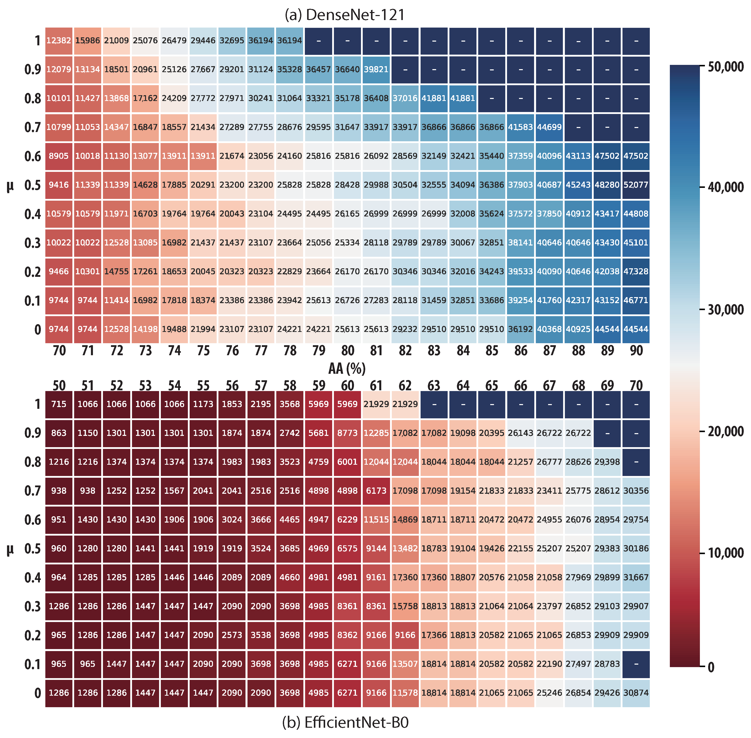
4.2. Evaluation of Gradient Filter

Before the comparison with baselines, the effect of the threshold for the gradient filter should be analyzed, i.e., the value of $\mu$. In general, $\mu$ controls the cosine similarity, and $\mu \in [-1,1]$, based on the fact that when the cosine similarity is negative, there exist opposite components of the two vectors. Thus, only non-negative $\mu$ is considered. As shown in Figure 2 and Figure 3, the performance of the two tested models with different $\mu$ is examined by using FOMAML.

Figure 2. Heat map of the communication cost required to reach different AAs in (a) DenseNet-121 and (b) EfficientNet-B0. Note that “-” indicates that the AA cannot be reached.

Figure 3. Overall distribution of AA under different $\mu$, where $\mu =0.6$ and evaluation without gradient filters are highlighted.

First, as shown in Figure 2, different communication costs and rounds are required to reach AAs as indicated by the x-axis. It can be seen that when $\mu =0.6$ is used, a more significant improvement in learning performance can be achieved, as ICMFed can save 3121.57% and 23.39% on average in DenseNet-121 and EfficientNet-B0, respectively. This shows the efficiency of the gradient filter in saving communication costs.

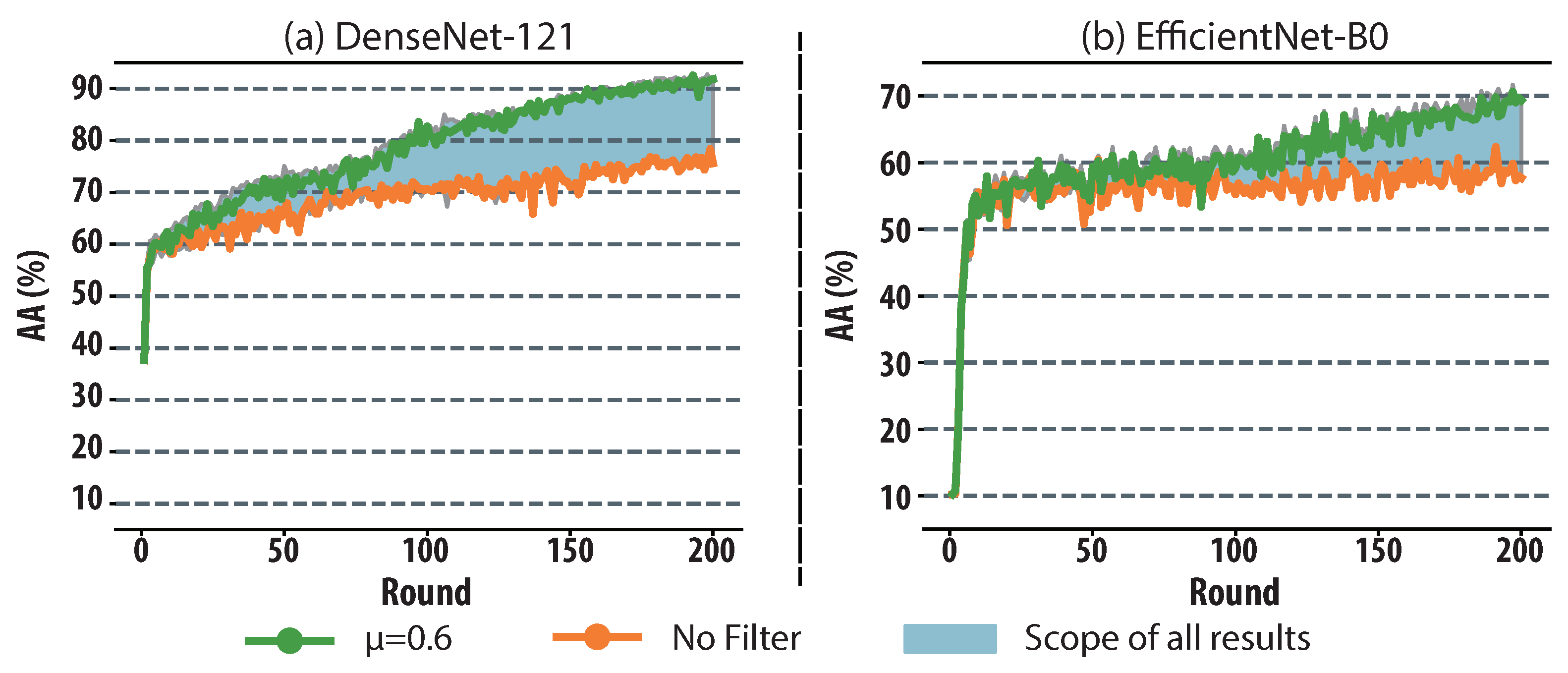
Moreover, as for learning stability, the AA curve under different $\mu$ is presented in Figure 3, in which the optimal results with $\mu =0.6$ and the basic result without gradient filters are highlighted, respectively. It shows that the maximum and average improvement in AA are 29.57% and 13.47% in DenseNet-121, and 20.38% and 7.97% in EfficientNet-B0, respectively. Such results show that the amount of information to be transmitted through the network can be significantly reduced in each learning round.

4.3. Evaluation of General Metrics

Based on the above analysis, $\mu =0.6$ is used by default and accordingly, the three general metrics are used to compare the proposed ICMFed with the baselines.

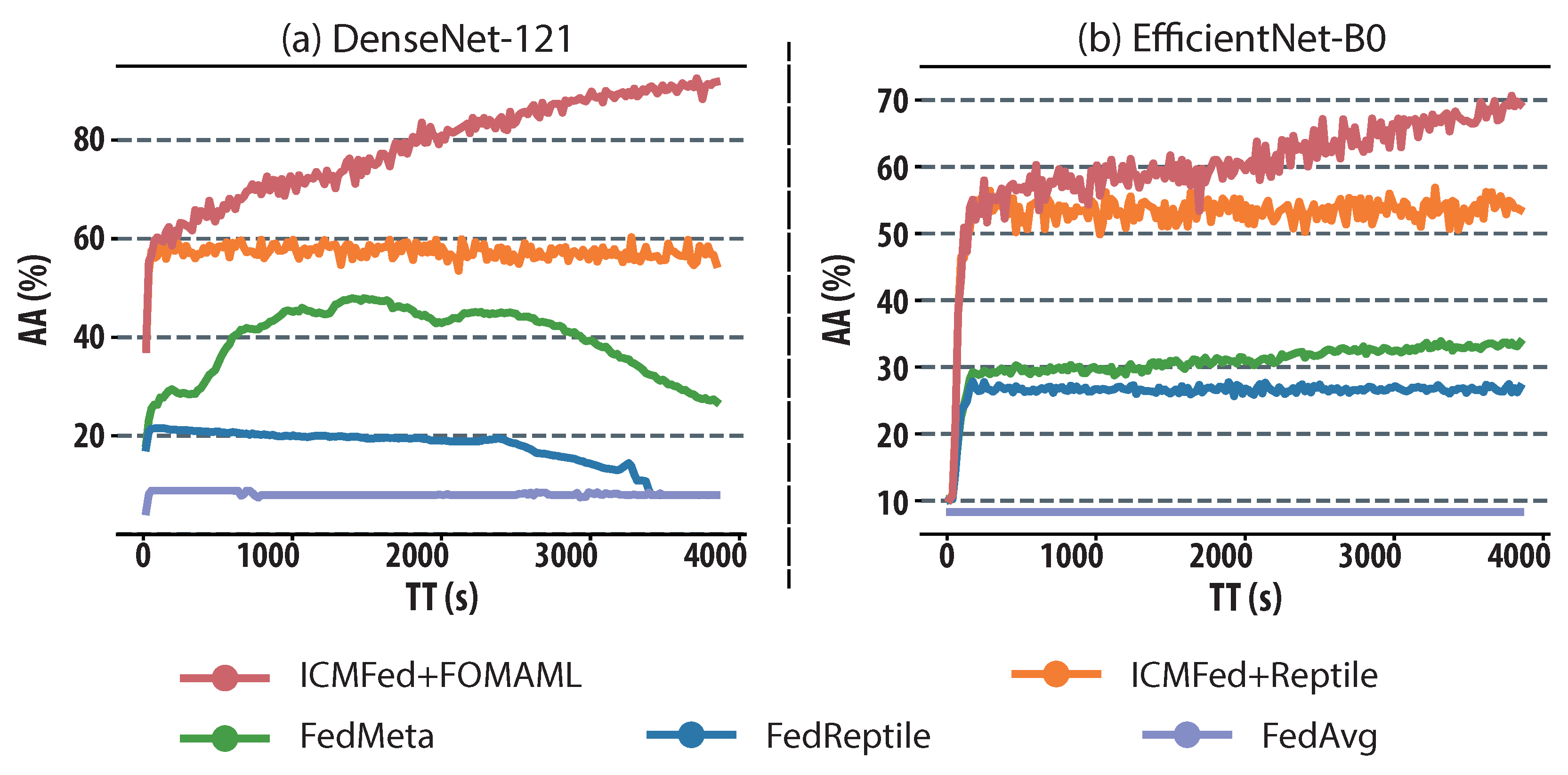
First, as shown in Figure 4, under the same configuration, all the methods can surpass the baseline FedAvg, and FedMeta outperforms FedReptile with a clear gap between their AA curves. Unsurprisingly, ICMFed with FOMAML and Reptile show the same results as illustrated in the compared results between FedMeta (using FOMAML) and FedReptile, and more importantly, regardless of models to be trained; ICMFed can significantly improve AA, i.e., on average by 105.81% and 95.46% with FOMAML and 265.08% and 99.32% with Reptile.

Figure 4. Relationship between AA and TT in (a) DenseNet-121 and (b) EfficientNet-B0.

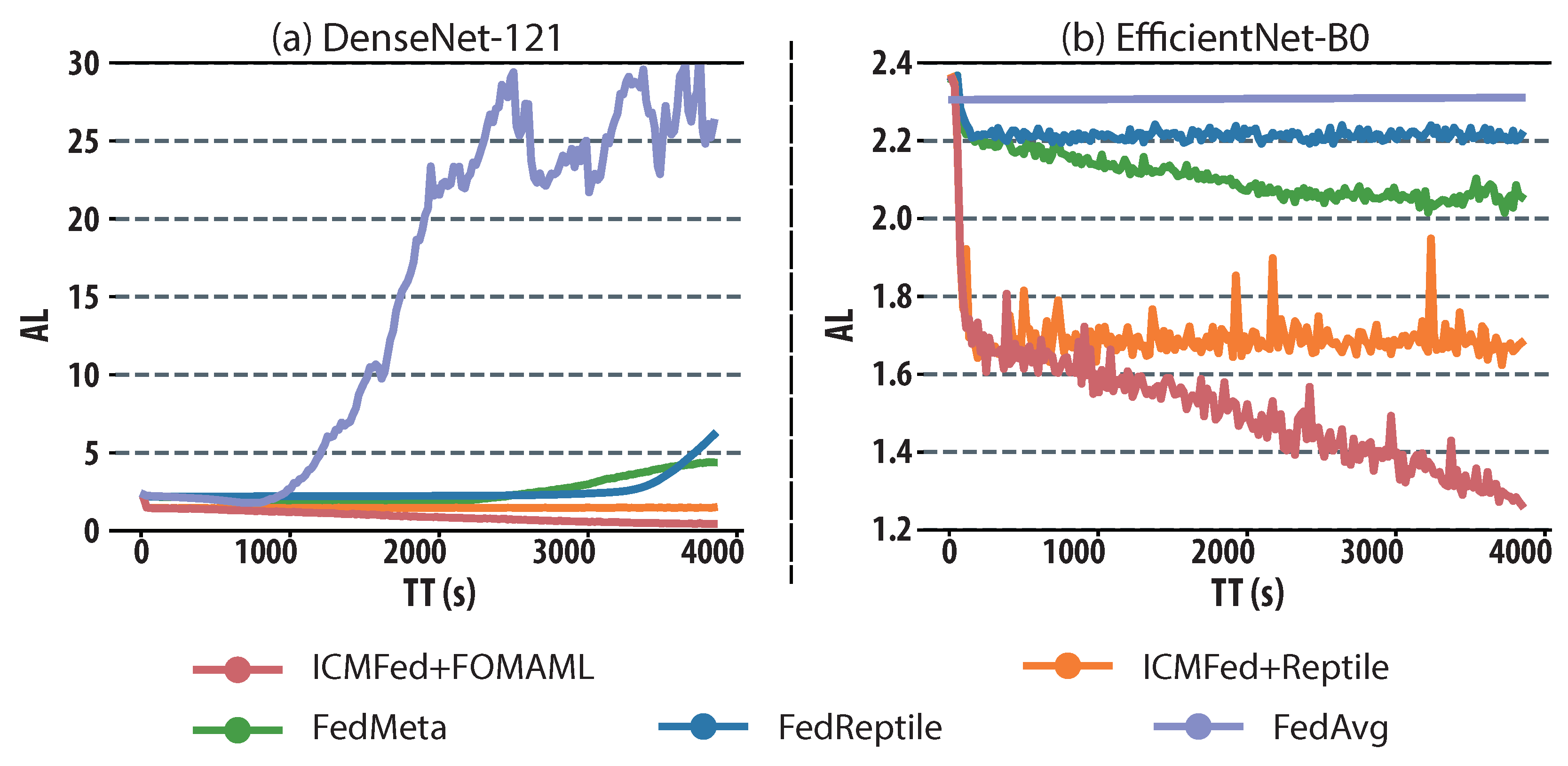
Second, as presented in Figure 5, ICMFed can boost AL by about 57.03% and 28.52% with FOMAML and 38.58% and 23.27% with Reptile, while comparing to the baselines. Specifically, as shown in Figure 5a, ICMFed can remediate the overfitting experienced in the baselines to train DenseNet-121. As shown in Figure 5b, even though the AL curves of two ICMFed variants fluctuate, it can still have the best performance compared to the baselines.

Figure 5. Relationship between AL and TT in (a) DenseNet-121 and (b) EfficientNet-B0.

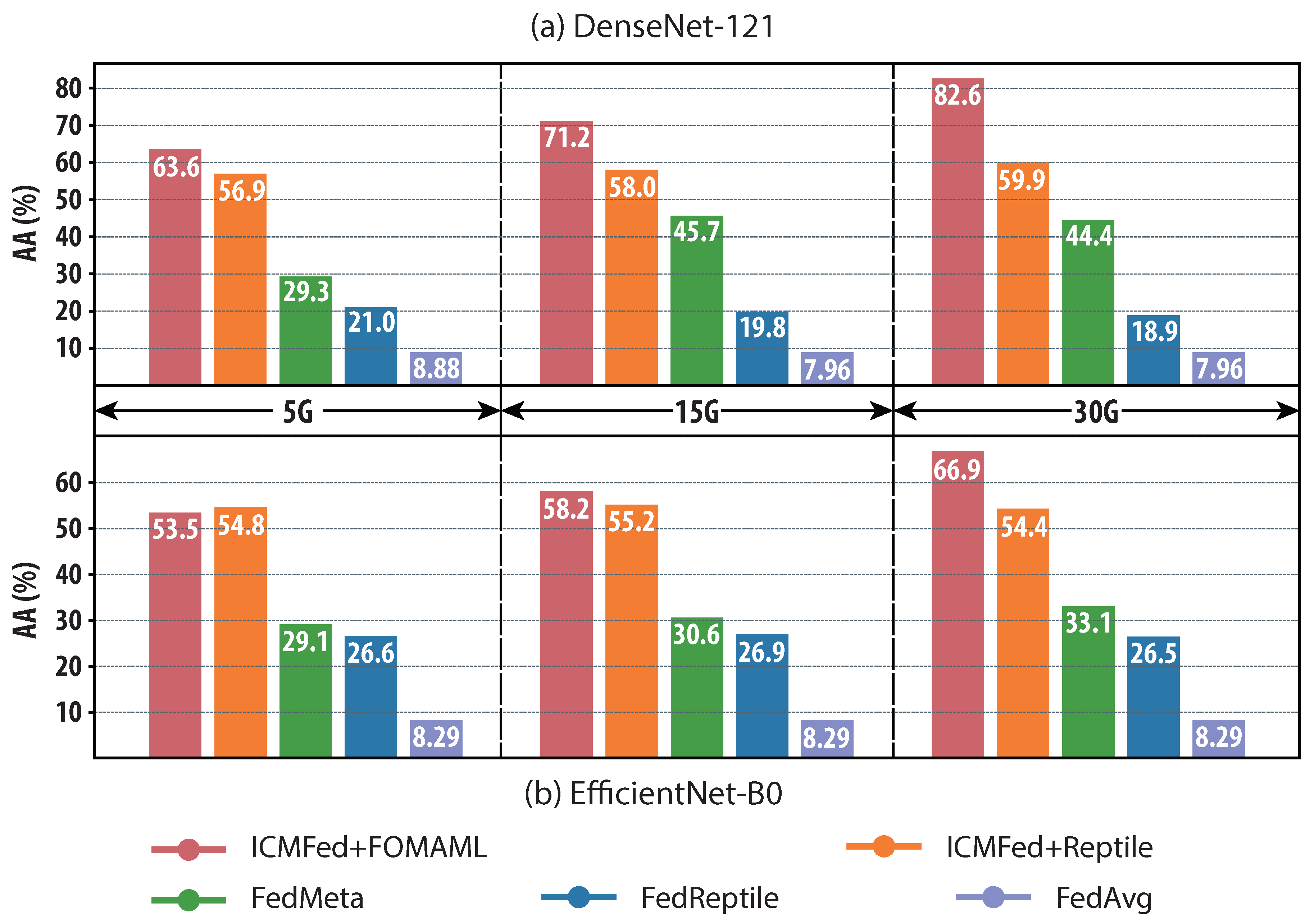
Finally, Figure 6 demonstrates AA reached with the specified communication cost for each evaluated method. Five gigabytes (GB), fifteen GB, and thirty GB are chosen as the three communication cost thresholds. In general, DenseNet-121 requires less cost than EfficientNet-B0 to reach a higher AA. For the three testing cases in DenseNet-121, ICMFed can improve the reached AA on average by 312.34%, 369.50%, and 453.33% with FOMAML and 269.06%, 282.73%, and 301.55% with Reptile, respectively. As for the three cases in EfficientNet-B0, ICMFed can improve the reached AA on average by 243.25%, 269.31%, and 320.84% with FOMAML and 251.67%, 250.53%, and 241.83% with Reptile, respectively. In summary, ICMFed can improve overall performance by 297.16%.

Figure 6. AA reached with the specified communication cost, namely, 5G, 15G, and 30G, in (a) DenseNet-121 and (b) EfficientNet-B0.

The above analyses show that compared to the baselines, ICMFed (especially the one equipped with FOMAML) can not only significantly reduce the communication cost but also dramatically improve the learning accuracy for both tested models.

4.4. Evaluation of Service-Quality Metrics

Based on the three service-quality metrics, the proposed ICMFed is further compared with the baselines. As illustrated in Table 5, in general, ICMFed with FOMAML is better than the one with Reptile, even though they can both outperform other methods. Specifically, while compared to the three baselines, ICMFed with FOMAML can enhance service quality by 193.46% in DenseNet-121 and 116.42% in EfficientNet-B0, which is 71.24% and 77.57% for Reptile. Note that SSQ of ICMFed is slightly lower in EfficientNet-B0, which can be interpreted as its slight sacrifice of stability for better service quality.

Table 5. Evaluation result of service-quality metrics.

Model	Metric	ICMFed+FOMAML	ICMFed+Reptile	FedMeta	FedReptile	FedAvg
DenseNet-121	BSQ	0.399 *	0.260${ }^{†}$	0.207	0.094	0.039
	ISQ	0.501	0.180	0.169	0.014	0.137
	SSQ	0.210	0.208	0.204	0.193	0.185
EfficientNet-B0	BSQ	0.356	0.287	0.172	0.142	0.043
	ISQ	0.340	0.247	0.186	0.146	0.081
	SSQ	0.208	0.207	0.209	0.205	0.171

* The best value among the compared methods is bolded. ${}^{†}$ The second best value among the compared methods is underlined.

In summary, an average improvement of 96.86% is achieved by ICMFed in service quality for both tested models.

4.5. Discussion

For experiment settings, the following two points are worth elaborating:

• Heterogeneous Setting. Even though the abovementioned settings do not include a specific section to describe the heterogeneous settings, there are three heterogeneous settings in our experimental scenario. First, in the State-Farm-Distracted-Driver-Detection dataset, there is heterogeneity across driver data, as shown in Table 3, and the clients are divided according to drivers to obtain data heterogeneity across clients. Second, random time delays for the clients are added to simulate heterogeneous communication conditions. Finally, during data increment, both the proportion of data growth and the probability of its occurrence may vary greatly between clients to simulate the heterogeneous data-aware process.
• Model Selection. To fairly evaluate the methods, DenseNet-121 and EfficientNet-B0 are selected to perform the experiments. These are chosen because they are classic and widely used models, and can achieve state-of-the-art performance in computer vision with a representative and indicative value [49,50]. They are also widely used in other works as testing models [51,52,53].

According to the above evaluations, the following observations can be drawn, namely:

• Gradient filters are helpful in optimizing both learning cost and accuracy. Gradient filters are originally designed to save communication costs. Since the amount of information to be updated is reduced, the filter may impact the overall learning accuracy. However, the results show that the usage of gradient filters will not affect the model performance, and instead, it can slightly improve AA by using an appropriate threshold $\mu$.
• Meta-learning is effective to support 3D tasks in a personalized context. Based on the fast adaptation enabled by the meta-model, meta-learning combined with FL, i.e., FM, can enable the personalization of local models to better support 3D. Moreover, by using dedicated strategies proposed by ICMFed, the performance can be significantly improved to support IFM, which is more realistic.
• ICMFed shows significant improvements compared to the baselines. According to the evaluation results in generic and service-quality metrics, ICMFed is cost-efficient to support IFM in 3D regardless of the models to be trained. Specifically, ICMFed equipped with FOMAML can outperform the one with Reptile under the same configuration.

5. Conclusions

To protect user privacy and gradually increasing process data, IFM is starting to be discussed to support 3D. In particular, four emerging challenges, i.e., data accumulation, communication optimization, data heterogeneity, and device heterogeneity, need to be addressed and hence, this paper proposes ICMFed, which can (1) achieve retention of knowledge by introducing a temporal factor associated with the batches created by sorting data created time-ascendingly in local training, (2) optimize the client–server interaction according to gradient filters of each model layer with communication costs reduced, (3) update the global model based on the weights measuring the differences of local updates in information richness to learn meta-learning efficiently, and (4) enhance 3D capability for each user based on the adaptation of the global meta-model to improve personalization.

According to the evaluation made on the State-Farm-Distracted-Driver-Detection dataset, ICMFed with FOMAML or Reptile can outperform the baselines to train both DenseNet-121 and EfficientNet-B0 models. Particularly, ICMFed can boost model accuracy by about 297.16% (when the target communication cost is reached), and improve service quality by about 96.86%.

In the future, first, the asynchronous mode of ICMFed will be studied to further improve the learning performance, especially the model update speed. Meanwhile, in asynchronous mode, the inference of global gradients on clients needs to be taken into account, i.e., due to the asynchronization, it cannot be inferred directly from the alterations between two adjacent rounds. In addition, the local gradients, whose creation time may vary, shall be aggregate-adaptive to remedy the impact of temporal difference. Finally, incentive mechanisms will be designed for ICMFed to attract more users to share their knowledge.

References

- Qin, L.; Li, Z.R.; Chen, Z.; Bill, M.A.; Noyce, D.A. Understanding driver distractions in fatal crashes: An exploratory empirical analysis. J. Saf. Res. 2019, 69, 23–31. [Google Scholar] [CrossRef] [PubMed]
- Wundersitz, L. Driver distraction and inattention in fatal and injury crashes: Findings from in-depth road crash data. Traffic Inj. Prev. 2019, 20, 696–701. [Google Scholar] [CrossRef] [PubMed]
- Lee, J.D.; Young, K.L.; Regan, M.A. Defining driver distraction. Driv. Distraction Theory Eff. Mitig. 2008, 13, 31–40. [Google Scholar]
- Hari, C.; Sankaran, P. Driver distraction analysis using face pose cues. Expert Syst. Appl. 2021, 179, 115036. [Google Scholar] [CrossRef]
- Aljasim, M.; Kashef, R. E2DR: A deep learning ensemble-based driver distraction detection with recommendations model. Sensors 2022, 22, 1858. [Google Scholar] [CrossRef]
- Li, G.; Yan, W.; Li, S.; Qu, X.; Chu, W.; Cao, D. A temporal–spatial deep learning approach for driver distraction detection based on EEG signals. IEEE Trans. Autom. Sci. Eng. 2021, 19, 2665–2677. [Google Scholar] [CrossRef]
- Fang, J.; Yan, D.; Qiao, J.; Xue, J.; Yu, H. DADA: Driver attention prediction in driving accident scenarios. IEEE Trans. Intell. Transp. Syst. 2021, 23, 4959–4971. [Google Scholar] [CrossRef]
- McMahan, B.; Moore, E.; Ramage, D.; Hampson, S.; y Arcas, B.A. Communication-efficient learning of deep networks from decentralized data. In Proceedings of the Artificial Intelligence and Statistics, PMLR, Fort Lauderdale, FL, USA, 20–22 April 2017; pp. 1273–1282. [Google Scholar]
- Li, T.; Sahu, A.K.; Talwalkar, A.; Smith, V. Federated learning: Challenges, methods, and future directions. IEEE Signal Process. Mag. 2020, 37, 50–60. [Google Scholar] [CrossRef]
- Shang, E.; Liu, H.; Yang, Z.; Du, J.; Ge, Y. FedBiKD: Federated Bidirectional Knowledge Distillation for Distracted Driving Detection. IEEE Internet Things J. 2023. [Google Scholar] [CrossRef]
- Javed, A.R.; Hassan, M.A.; Shahzad, F.; Ahmed, W.; Singh, S.; Baker, T.; Gadekallu, T.R. Integration of blockchain technology and federated learning in vehicular (iot) networks: A comprehensive survey. Sensors 2022, 22, 4394. [Google Scholar] [CrossRef]
- Novikova, E.; Fomichov, D.; Kholod, I.; Filippov, E. Analysis of privacy-enhancing technologies in open-source federated learning frameworks for driver activity recognition. Sensors 2022, 22, 2983. [Google Scholar] [CrossRef] [PubMed]
- Feng, T.; Wang, M.; Yuan, H. Overcoming Catastrophic Forgetting in Incremental Object Detection via Elastic Response Distillation. In Proceedings of the IEEE/CVF Conference on Computer Vision and Pattern Recognition, New Orleans, LA, USA, 18–24 June 2022; pp. 9427–9436. [Google Scholar]
- Fallah, A.; Mokhtari, A.; Ozdaglar, A. Personalized federated learning: A meta-learning approach. arXiv 2020, arXiv:2002.07948. [Google Scholar]
- Chen, F.; Luo, M.; Dong, Z.; Li, Z.; He, X. Federated meta-learning with fast convergence and efficient communication. arXiv 2018, arXiv:1802.07876. [Google Scholar]
- Hussain, M.A.; Huang, S.A.; Tsai, T.H. Learning with Sharing: An Edge-optimized Incremental Learning Method for Deep Neural Networks. IEEE Trans. Emerg. Top. Comput. 2022. [Google Scholar] [CrossRef]
- Konečnỳ, J.; McMahan, H.B.; Yu, F.X.; Richtárik, P.; Suresh, A.T.; Bacon, D. Federated learning: Strategies for improving communication efficiency. arXiv 2016, arXiv:1610.05492. [Google Scholar]
- Nori, M.K.; Yun, S.; Kim, I.M. Fast federated learning by balancing communication trade-offs. IEEE Trans. Commun. 2021, 69, 5168–5182. [Google Scholar] [CrossRef]
- Nishio, T.; Yonetani, R. Client selection for federated learning with heterogeneous resources in mobile edge. In Proceedings of the ICC 2019-2019 IEEE International Conference on Communications (ICC), Shanghai, China, 20–24 May 2019; pp. 1–7. [Google Scholar]
- AbdulRahman, S.; Tout, H.; Ould-Slimane, H.; Mourad, A.; Talhi, C.; Guizani, M. A survey on federated learning: The journey from centralized to distributed on-site learning and beyond. IEEE Internet Things J. 2020, 8, 5476–5497. [Google Scholar] [CrossRef]
- Lu, Y.; Huang, X.; Zhang, K.; Maharjan, S.; Zhang, Y. Blockchain empowered asynchronous federated learning for secure data sharing in internet of vehicles. IEEE Trans. Veh. Technol. 2020, 69, 4298–4311. [Google Scholar] [CrossRef]
- Wei, G.; Li, X. Knowledge Lock: Overcoming Catastrophic Forgetting in Federated Learning. In Proceedings of the Pacific-Asia Conference on Knowledge Discovery and Data Mining, Chengdu, China, 16–19 May 2022; pp. 601–612. [Google Scholar]
- Dong, J.; Wang, L.; Fang, Z.; Sun, G.; Xu, S.; Wang, X.; Zhu, Q. Federated class-incremental learning. In Proceedings of the IEEE/CVF Conference on Computer Vision and Pattern Recognition, New Orleans, LA, USA, 18–24 June 2022; pp. 10164–10173. [Google Scholar]
- Lin, T.; Kong, L.; Stich, S.U.; Jaggi, M. Ensemble distillation for robust model fusion in federated learning. Adv. Neural Inf. Process. Syst. 2020, 33, 2351–2363. [Google Scholar]
- Yoon, J.; Jeong, W.; Lee, G.; Yang, E.; Hwang, S.J. Federated continual learning with weighted inter-client transfer. In Proceedings of the International Conference on Machine Learning, PMLR, Virtual, 18–24 July 2021; pp. 12073–12086. [Google Scholar]
- Le, J.; Lei, X.; Mu, N.; Zhang, H.; Zeng, K.; Liao, X. Federated continuous learning with broad network architecture. IEEE Trans. Cybern. 2021, 51, 3874–3888. [Google Scholar] [CrossRef]
- Qin, Z.; Li, G.Y.; Ye, H. Federated learning and wireless communications. IEEE Wireless Commun. 2021, 28, 134–140. [Google Scholar] [CrossRef]
- Liu, S.; Chen, Q.; You, L. Fed2a: Federated learning mechanism in asynchronous and adaptive modes. Electronics 2022, 11, 1393. [Google Scholar] [CrossRef]
- Chen, Y.; Ning, Y.; Slawski, M.; Rangwala, H. Asynchronous online federated learning for edge devices with non-iid data. In Proceedings of the 2020 IEEE International Conference on Big Data (Big Data), Atlanta, GA, USA, 10–13 December 2020; pp. 15–24. [Google Scholar]
- You, L.; Liu, S.; Chang, Y.; Yuen, C. A triple-step asynchronous federated learning mechanism for client activation, interaction optimization, and aggregation enhancement. IEEE Internet Things J. 2022, 9, 24199–24211. [Google Scholar] [CrossRef]
- Mhaisen, N.; Abdellatif, A.A.; Mohamed, A.; Erbad, A.; Guizani, M. Optimal user-edge assignment in hierarchical federated learning based on statistical properties and network topology constraints. IEEE Trans. Netw. Sci. Eng. 2021, 9, 55–66. [Google Scholar] [CrossRef]
- Sattler, F.; Wiedemann, S.; Müller, K.R.; Samek, W. Robust and communication-efficient federated learning from non-iid data. IEEE Trans. Neural Netw. Learn. Syst. 2019, 31, 3400–3413. [Google Scholar] [CrossRef]
- Ma, X.; Zhang, J.; Guo, S.; Xu, W. Layer-wised model aggregation for personalized federated learning. In Proceedings of the IEEE/CVF Conference on Computer Vision and Pattern Recognition, New Orleans, LA, USA, 18–24 June 2022; pp. 10092–10101. [Google Scholar]
- Lian, Z.; Wang, W.; Su, C. COFEL: Communication-efficient and optimized federated learning with local differential privacy. In Proceedings of the ICC 2021-IEEE International Conference on Communications, Montreal, QC, Canada, 14–23 June 2021; pp. 1–6. [Google Scholar]
- Lian, Z.; Wang, W.; Huang, H.; Su, C. Layer-based communication-efficient federated learning with privacy preservation. IEICE Trans. Inf. Syst. 2022, 105, 256–263. [Google Scholar] [CrossRef]
- Finn, C.; Abbeel, P.; Levine, S. Model-agnostic meta-learning for fast adaptation of deep networks. In Proceedings of the International Conference on Machine Learning, PMLR, Sydney, Australia, 6–11 August 2017; pp. 1126–1135. [Google Scholar]
- Nichol, A.; Achiam, J.; Schulman, J. On first-order meta-learning algorithms. arXiv 2018, arXiv:1803.02999v3. [Google Scholar]
- Nichol, A.; Schulman, J. Reptile: A scalable metalearning algorithm. arXiv 2018, arXiv:1803.02999v1. [Google Scholar]
- Jiang, Y.; Konečnỳ, J.; Rush, K.; Kannan, S. Improving federated learning personalization via model agnostic meta learning. arXiv 2019, arXiv:1909.12488. [Google Scholar]
- Qu, H.; Liu, S.; Li, J.; Zhou, Y.; Liu, R. Adaptation and Learning to Learn (ALL): An Integrated Approach for Small-Sample Parking Occupancy Prediction. Mathematics 2022, 10, 2039. [Google Scholar] [CrossRef]
- Qu, H.; Liu, S.; Guo, Z.; You, L.; Li, J. Improving Parking Occupancy Prediction in Poor Data Conditions Through Customization and Learning to Learn. In Proceedings of the Knowledge Science, Engineering and Management: 15th International Conference, KSEM, Singapore, 6–8 August 2022; pp. 159–172. [Google Scholar]
- Li, W.; Wang, S. Federated meta-learning for spatial-temporal prediction. Neural Comput. Appl. 2022, 34, 10355–10374. [Google Scholar] [CrossRef]
- Wu, W.; He, L.; Lin, W.; Mao, R.; Maple, C.; Jarvis, S. SAFA: A semi-asynchronous protocol for fast federated learning with low overhead. IEEE Trans. Comp. 2020, 70, 655–668. [Google Scholar] [CrossRef]
- Huang, T.; Lin, W.; Wu, W.; He, L.; Li, K.; Zomaya, A.Y. An efficiency-boosting client selection scheme for federated learning with fairness guarantee. IEEE Trans. Parallel Distrib. Syst. 2020, 32, 1552–1564. [Google Scholar] [CrossRef]
- Li, D.; Li, J.; Fan, Y.; Lu, G.; Ge, J.; Liu, X. Printed label defect detection using twice gradient matching based on improved cosine similarity measure. Expert Syst. Appl. 2022, 204, 117372. [Google Scholar] [CrossRef]
- Yu, T.; Kumar, S.; Gupta, A.; Levine, S.; Hausman, K.; Finn, C. Gradient surgery for multi-task learning. Adv. Neural Inf. Process. Syst. 2020, 33, 5824–5836. [Google Scholar]
- Huang, G.; Liu, Z.; Van Der Maaten, L.; Weinberger, K.Q. Densely connected convolutional networks. In Proceedings of the IEEE Conference on Computer Vision and Pattern Recognition, Honolulu, HI, USA, 21–26 July 2017; pp. 4700–4708. [Google Scholar]
- Tan, M.; Le, Q. Efficientnet: Rethinking model scaling for convolutional neural networks. In Proceedings of the International Conference on Machine Learning, PMLR, Long Beach, CA, USA, 9–15 June 2019; pp. 6105–6114. [Google Scholar]
- Nandhini, S.; Ashokkumar, K. An automatic plant leaf disease identification using DenseNet-121 architecture with a mutation-based henry gas solubility optimization algorithm. Neural Comput. Appl. 2022, 34, 5513–5534. [Google Scholar] [CrossRef]
- Yang, B.; Bender, G.; Le, Q.V.; Ngiam, J. Condconv: Conditionally parameterized convolutions for efficient inference. Adv. Neural Inf. Process. Syst. 2019, 32. [Google Scholar]
- Chetoui, M.; Akhloufi, M.A. Automated Detection of COVID-19 Cases using Recent Deep Convolutional Neural Networks and CT images. In Proceedings of the 2021 43rd Annual International Conference of the IEEE Engineering in Medicine & Biology Society (EMBC), Virtual, 1–5 November 2021; pp. 3297–3300. [Google Scholar]
- Oztekin, F.; Katar, O.; Sadak, F.; Yildirim, M.; Cakar, H.; Aydogan, M.; Ozpolat, Z.; Talo Yildirim, T.; Yildirim, O.; Faust, O.; et al. An Explainable Deep Learning Model to Prediction Dental Caries Using Panoramic Radiograph Images. Diagnostics 2023, 13, 226. [Google Scholar] [CrossRef]
- Jana, S.; Middya, A.I.; Roy, S. Participatory Sensing Based Urban Road Condition Classification using Transfer Learning. Mob. Netw. Appl. 2023, 45, 1–17. [Google Scholar] [CrossRef]