A Passive-Constrained Observer and Controller Applied to an In-Wheel Synchronous Machine Implemented on a Fixed-Point DSP

Abstract

In this paper, we describe a passivity-based control (PBC) approach for in-wheel permanent magnet synchronous machines that expands on the conventional passivity-based controller. We derive the controller and observer parameter constraints in order to maintain the passivity of the interconnected system and thus improve the control system’s robustness to varying loads and plant parameters. The advantages of the proposed PBC technique are demonstrated in contrast with conventional PBC. The control technique is implemented on an electronic development board equipped with a fixed-point digital signal processor and coupled to a gallium nitride voltage source inverter and 350 W electric machine. Test bench results and numerical simulations in Matlab-Simulink demonstrate the control performance and behaviour under varying loads and parameters.

1. Introduction

E-mobility is one of the most promising approaches to sustainable transportation. Vehicles with electric drive trains have a lower environmental impact as well as improved vehicle performance. Significant progress has been made in the electrification of drive trains in recent years. Although it is still in its early stages, electromobility has large market potential because governments have begun to support customers by lowering tax rates and constructing the necessary infrastructure. Energy storage technology advancements, on the other hand, are critical for the future of electrical propulsion drive trains. Electrical power trains are commonly powered by induction machines, externally excited synchronous machines, or permanent magnet synchronous machines. Despite their higher price, the latter are preferred due to their reliability and higher power density. A special case of permanent magnet synchronous machine is the direct current synchronous machine. Because the stator windings are concentrated rather than distributed, they become less expensive than current alternative counterparts. The winding process in the latter case is easier to implement in large-scale production. They are mass-produced items. The multi-pole in-wheel synchronous machine (IWSM) is an outrunner permanent magnet synchronous machine with 30 or more magnetic poles mounted on a ring or sleeve on the outside of the stator coils. IWSMs offer adequate power density for mobile robots and tiny and compact e-vehicles, such as e-scooters, electric wheelchairs, and electric bicycles, etc. IWSMs can be exposed to unnatural, harsh climates (e.g., planets exploration). The Martian research rovers Opportunity and Spirit, which were launched in 2004, endured dust storms, temperature variations ranging from −125 to +25 °C, vibrations, and mechanical stresses. These mobile robots are equipped with similar electrical machines.

Several initiatives have been taken to design control algorithms that improve dynamic efficiency and robustness. We highlight some of the key accomplishments in this field. The authors in [1] provide a sliding mode speed control approach. Adaptive control is utilized in some circumstances, such as when the parameters of an electrical machine are prone to large variation [2]. The authors propose an adaptive fuzzy controller in [3]. Phase advance techniques can be used to expand the speed range of BLDCs [4]. Researchers propose finite-set MPCs for BLDC and PMSM devices in [5,6]. Passive electrical machines use the passivity characteristics of rotating machines to govern the dissipated power [7,8]. The authors discuss a predictive flux regulator with virtual vectors in [9]. In [10], a passivity-based MPC without state or input limitations is studied. Several studies have considered introducing a dissipation-based limitation into model predictive regulators [11,12,13]. Current interest in nonlinear control theory has been focused on passivity-based control (PBC) due to its robustness, good performance, and relatively simple design. Authors in [14] discuss the principles of a mixed controller–observer strategy where the controlled variables are voltages across machine phases. The algorithm is sensorless to some extent, without the need for measuring phase currents or rotor speed. An adaptive law reconstructs rotor velocity and stator currents; however, the method is based on a PI speed controller and provides advances in the area of parameter robustness [14]. Another PBC strategy designed in the $dq$ rotor reference frame is used in conjunction with an active disturbance rejection controller in the outer loop [15]. The extended observer can be used to estimate the total internal and external disturbances [15]. In order to increase the robustness to parameter variations, we included both electrical and mechanical disturbance observers in our proposed method. PBC is used in power converters [16,17]. A control algorithm based on a port-controlled Hamiltonian structure with adaptive immersion and invariance schemes is proposed for the $dq$ reference frame. In their design, the authors take into account how the phase resistance and friction coefficient change over time [18]. A conventional PBC design is described by the authors in [19]. We considered parameter variations in this research since we noticed steady-state errors in the classic PBC and we derived the conditions to maintain the passivity property of the inter-connected controller–observer. In the rotor reference frame, a PBC method based on a port-controlled Hamiltonian structure has been devised [20]. The approach has some similarities with [18] and paves the path for many advancements in port-controlled Hamiltonian structures. In the construction of a PBC sensorless control scheme, an observer is utilized to assess the motor position and velocity. The technique employs an incremental controller to guarantee that there is no steady-state error [21]. In this context, our findings suggest a control technique based on passivity-based control with guaranteed passivity of the controller–observer. An IWSM in motor mode is being considered. The control strategy is designed using the Euler-Lagrange (EL) mathematical model of the electrical machine. As can be observed, the plant defines some specific passive mappings, and as a result, the dynamics are considered as two distinct EL passive subsystems: mechanical and electrical. Feedforward commands ensure tolerance to parameter variations. As can be observed, the plant defines some specific passive mappings, and as a result, the dynamics are considered as two distinct EL passive subsystems: mechanical and electrical. The mechanical subsystem’s dynamics are handled as passive disturbances of the electrical subsystem. A damping term is introduced to strengthen the electrical dynamics’ passivity. Furthermore, current tracking is accomplished by re-modelling the internal closed-loop energy. Finally, control laws are established to assure internal stability with global current and speed tracking. The control strategy proposed in this work is compared against a strategy that relies on conventional PBC and PI controllers. The proposed control structure has better dynamic performances and is more effective in terms of robustness to parameter fluctuations.

This paper continues with Section 2, where we introduce the mathematical model of the process used in the design of the controller. In Section 3, we define the passivity of the IWSM and discuss the concept of the controller. We impose desired dissipating and energy-storing functions. We provide the description of the joint controller–observer and argue the conditions for preserving the passivity property of the interconnected system. In Section 4, we describd the hardware setup. In Section 5, we implement the control structure on a fixed-point DSP which controls a gallium-nitride voltage source inverter (VSI) connected to the IWSM. We evaluate the control performance on a 350 W power test bench along with numerical simulations in Matlab-Simulink.

2. Mathematical Modeling in Stationary Frame

In order to obtain the electrical and mechanical equilibrium equations of the synchronous permanent magnet machine, we apply the Hamilton principle, commonly referred to as the ‘least action’ principle [22]. If only conservative forces are acting on the system, then the dynamics path $q\left(t\right)={\left[q_e{\left(t\right)}^T{q}_m\left(t\right)\right]}^T$ of the electrical machine will evolve from one configuration $q\left(t_1\right)$ to another $q\left(t_2\right)$ in such a way that it minimizes the cost functional (1):

$$I={\int }_{t_1}^{t_2}L(q\left(t\right),\dot{q}\left(t\right),t)dt,$$

(1)

where L is the Lagrangian and is defined as follows [22,23]:

$$L(q\left(t\right),\dot{q}\left(t\right),t)=K(q_e\left(t\right),{\dot{q}}_e\left(t\right),q_m\left(t\right))-V\left(q_m\left(t\right)\right)$$

(2)

In the previous equation, K denotes the total kinetic energy, and V denotes the total potential energy. The charge velocities are denoted by ${\dot{q}}_e\left(t\right)={\left[i_{\alpha }{i}_{\beta }\right]}^T$, which are the stator currents in the stationary frame. The mechanical angle is denoted by $q_m\left(t\right)$, and the mechanical angular frequency is denoted by ${\dot{q}}_m\left(t\right)$. $q_e\left(t\right)$ defines the charge potential. A problem involving optimization is formulated. The actual path that defines the dynamics of the synchronous permanent magnet machine is the solution $q\left(t\right)={\left[q_e\left(t\right)q_m\left(t\right)\right]}^t$, which minimizes the cost functional (1). This solution satisfies the set of nonlinear ordinary differential equations, referred to as Euler-Lagrange equations:

$$\frac{d}{dt}\frac{\partial L}{\partial \dot{q}}-\frac{\partial L}{\partial q}=0,$$

(3)

where q and $\dot{q}$ are standard notations for the generalized coordinates and velocities, respectively. Non-conservative forces and dissipative effects act on the electrical machine and are modelled as external disturbances Q:

$$Q=u-\frac{\partial F}{\partial \dot{q}}$$

(4)

The EL equation of the system affected by disturbance Q is [23]

$$\frac{d}{dt}\frac{\partial L}{\partial \dot{q}}-\frac{\partial L}{\partial q}=Q$$

(5)

In the previous equation, the input signal is $u={\left[u_e^T{u}_m\right]}^T$. The input voltage vector at the input of the process is $u_e={\left[u_{\alpha }{u}_{\beta }\right]}^T$ and $u_m=-T_l$ is the load torque. The external disturbance is defined by the electrical and mechanical counterparts $Q={\left[Q_e^T{Q}_m\right]}^T$. The dissipative forces are defined by $-\partial F/\partial \dot{q}$. The Rayleigh quadratic dissipation function is denoted by $F\left(\dot{q}\right)$:

$$F\left(\dot{q}\right)=\frac{1}{2}{\dot{q}}_e^T{R}_e{\dot{q}}_e+\frac{1}{2}{r}_m{\dot{q}}_m^2,$$

(6)

where matrix $R_e$ is defined by (7) and models the electrical resistance of the stator windings, while $r_m$ models the viscous friction coefficient at the shaft bearings.

$$R_e=diag\{r_s,r_s\}$$

(7)

2.1. Deriving Motion Equations from an Energy Model

The magnetic field co-energy of the synchronous permanent magnet machine is defined as follows [23]:

$$K_e^{\prime }({\dot{q}}_e,q_m)=\sum _{i=1}^2{\int }_0^{{\dot{q}}_i}{\lambda }_i\left({\dot{q}}_i\right)d{\dot{q}}_i$$

(8)

Consequently, $\lambda ={\left[{\lambda }_{\alpha }{\lambda }_{\beta }\right]}^t$ represents the flux linkage of stationary frame components:

$$\lambda =D_e\left(q_m\right){\dot{q}}_e+\mu \left(q_m\right)$$

(9)

Substituting (9) into (8) yields

$$K_e^{\prime }({\dot{q}}_e,q_m)=\frac{1}{2}{\dot{q}}_e^T{D}_e\left(q_m\right){\dot{q}}_e+{\mu }^T\left(q_m\right){\dot{q}}_e$$

(10)

The permanent magnet flux linkage components in the stator frame are defined:

$$\mu \left(q_m\right)={\lambda }_{pm}\left[\begin{array}{c}cos\left(p_p{q}_m\right)\\ sin\left(p_p{q}_m\right)\end{array}\right],$$

(11)

where ${\lambda }_{pm}$ is the flux amplitude of the permanent magnet and $p_p$ is the number of pole pairs. Finally, $D_e\left(q_m\right)=D_e^t\left(qm\right)>0$ represents the inductance matrix in $\alpha \beta$ coordinates and is defined by

$$D_e\left(q_m\right)=\left[\begin{array}{cc}{\overline{L}}_s-\Delta L_{s}cos\left(2p_p{q}_m\right),& -\Delta L_{s}sin\left(2p_p{q}_m\right)\\ -\Delta L_{s}sin\left(2p_p{q}_m\right),& {\overline{L}}_s+\Delta L_{s}cos\left(2p_p{q}_m\right)\end{array}\right],$$

(12)

where $\Delta L_s=\frac{1}{2}(L_q-L_d)$ is the inductance variations driven by saliency effects and ${\overline{L}}_s=\frac{1}{2}(L_d+L_q)$ is the average inductance owing to air gap flux. We simplify the control problem considering that the cogging torque is zero and thus potential energy is $V\left(q_m\right)=0$ (cogging torque could be higher at low speeds depending on the air gap). The mechanical kinetic energy is the following [23]:

$$K_m^{\prime }\left({\dot{q}}_m\right)=\frac{1}{2}{D}_m{\dot{q}}_m^2$$

(13)

and the rotor’s moment of inertia is $D_m>0$. From (2), (10), and (13), we obtain the Lagrangian of the electrical machine:

$$L({\dot{q}}_e,{\dot{q}}_m,q_m)=\frac{1}{2}{\dot{q}}_e^T{D}_e\left(q_m\right){\dot{q}}_e+{\mu }^T\left(q_m\right){\dot{q}}_e+\frac{1}{2}{D}_m{\dot{q}}_m^2$$

(14)

Substituting (14) in (5) yields the equation system describing the dynamics of the electrical subsystem (15) and the equation of the mechanical subsystem (16):

$$D_e\left(q_m\right){\ddot{q}}_e+W_p\left(q_m\right){\dot{q}}_m{\dot{q}}_e+W_q\left(q_m\right){\dot{q}}_m+R_e{\dot{q}}_e=u_e$$

(15)

$$D_m{\ddot{q}}_m-T_e({\dot{q}}_e,q_m)+r_m{\dot{q}}_m=u_m,$$

(16)

where $W_p$ and $W_q$ are defined as

$$W_p\left(q_m\right)=\frac{\partial D_e\left(q_m\right)}{\partial q_m}$$

(17)

$$W_q\left(q_m\right)=\frac{\partial \mu \left(q_m\right)}{\partial q_m}$$

(18)

Furthermore, the generated electromagnetic is obtained from the Lagrangian (14) as

$$T_e=\frac{\partial L({\dot{q}}_e,{\dot{q}}_m,q_m)}{\partial q_m}=\frac{1}{2}{\dot{q}}_e^T\frac{\partial D_e\left(q_m\right)}{\partial q_m}{\dot{q}}_e+{\left(\frac{\partial \mu \left(q_m\right)}{\partial q_m}\right)}^T{\dot{q}}_e$$

(19)

Figure 1 summarizes the model structure containing the electrical and mechanical subsystems and the associated inputs and outputs.

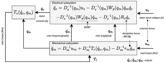
Figure 1. Illustration of the electrical machine model.

2.2. Passivity Property of the Process

Permanent magnet synchronous machines are passive systems with passive maps defined between the input $u={\left[u_e^T{u}_m\right]}^t$ and the output $\dot{q}={\left[{\dot{q}}_e^T{\dot{q}}_m\right]}^t$. The total energy determined by the Hamiltonian $H(q\left(t\right),\dot{q}\left(t\right),t)$ is

$$H(q\left(t\right),\dot{q}\left(t\right),t)=K(q_e\left(t\right),{\dot{q}}_e\left(t\right),q_m\left(t\right))+V\left(q_m\left(t\right)\right)$$

(20)

From (20), given that $V\left(qm\right)=0$, the total amount of energy is obtained:

$$H({\dot{q}}_e,{\dot{q}}_m,q_m)=\frac{1}{2}{\dot{q}}_e^T{D}_e\left(q_m\right){\dot{q}}_e+{\mu }^T\left(q_m\right){\dot{q}}_e+\frac{1}{2}{D}_m{\dot{q}}_m^2$$

(21)

From (21), the power balance equation is obtained by taking the time derivative of H:

$$\frac{dH}{dt}=\frac{\partial H}{\partial {\dot{q}}_e}{\ddot{q}}_e+\frac{\partial H}{\partial {\dot{q}}_m}{\ddot{q}}_m+\frac{\partial H}{\partial q_m}{\dot{q}}_m$$

(22)

Calculating the partial derivatives of H yields the expression for the power supplied to the energy-storing components of the electrical machine:

$$\dot{H}={\dot{q}}_e^T{D}_e\left(q_m\right){\ddot{q}}_e+{\mu }^T\left(q_m\right){\ddot{q}}_e+D_m{\dot{q}}_m{\ddot{q}}_m+{\dot{q}}_m{W}_q\left(q_m\right){\dot{q}}_e$$

By multiplying (15) and (16) with the current vector ${\dot{q}}_e$ and with the load torque $T_l$, respectively, and then substituting the results into (23), the power balance is obtained:

$$\frac{dH}{dt}={\dot{q}}^{T}u-{\dot{q}}^{T}Rq+\frac{d}{dt}\left({\mu }^T\left(q_m\right){\dot{q}}_e\right)$$

(23)

By integrating (23) over time, we obtain the energy equilibrium equation:

$$\begin{array}{c}\hfill \underset{\mathrm{stored}\mathrm{energy}}{\underbrace{H\left(T\right)-H\left(0\right)}}=\underset{\mathrm{supplied}\mathrm{energy}}{\underbrace{{\int }_0^T{\dot{q}}^{T}udt+{\mu }^T{\dot{q}}_e{|}_0^T}}-\underset{\mathrm{dissipated}\mathrm{energy}}{\underbrace{{\int }_0^T{\dot{q}}^{T}R\dot{q}dt}}\end{array}$$

(24)

In the previous equation, the positive definiteness of $R=diag\{R_e,r_m\}>0$ indicates that the stored energy is not greater than the supplied energy. It is thus defined as a passive map from the input u to the output $\dot{q}$.

3. Stator Frame Currents Controller

The passivity controller achieves the control goal by imposing the passivity property on the closed-loop system. This is accomplished by assigning desired dissipation and storage functions to the closed-loop system.

The mechanical dynamics (16) are regarded as a passive disturbance of the electrical subsystem, whereas the electrical subsystem is regarded as the system to be controlled.

The passivity of the electrical machine is straightened to strict passivity by injecting an additional command with dissipating factor $\mathsf{\Lambda }=diag({\lambda }_{\alpha },{\lambda }_{\beta })$. The mapping from $u_e$ to ${\dot{q}}_e$ is strictly passive if the input of the process is $u_e=v-\mathsf{\Lambda }(q_m,{\dot{q}}_m){\dot{q}}_e+W_p\left(q_m\right){\dot{q}}_m{\dot{q}}_e+W_q\left(q_m\right){\dot{q}}_m$. This leads to the closed-loop system defined by

$$v=D_e\left(q_m\right){\ddot{q}}_e+\left[R_e+\mathsf{\Lambda }(q_m,{\dot{q}}_e)\right]{\dot{q}}_e$$

(25)

Equation (25) defines the linear dynamics of the process, now decoupled from the permanent magnetic circuit with the convergence rate raised by $\mathsf{\Lambda }$. The power supplied to the magnetic field of the inductances becomes $\dot{H}={\dot{q}}_e^{T}v-{\dot{q}}_e^T\left[R_e+\mathsf{\Lambda }(q_m,{\dot{q}}_m)\right]{\dot{q}}_e$. Time integration of the power balance equation leads to the following energy equilibrium equation:

$$\underset{\mathrm{stored}\mathrm{energy}}{\underbrace{H\left(T\right)-H\left(0\right)}}=\underset{\mathrm{supplied}\mathrm{energy}}{\underbrace{{\int }_0^T{\dot{q}}_e^{T}vdt}}-\underset{\mathrm{dissipated}\mathrm{energy}}{\underbrace{{\int }_0^T{\dot{q}}_e^T\left[R_e+\mathsf{\Lambda }(q_m,{\dot{q}}_m)\right]{\dot{q}}_{e}dt}}$$

(26)

In practice, the permanent magnet flux $\mu$ varies with temperature, and the inductance with the amplitude of the current and with the electrical angle $p_p·q_m$. Therefore, $W_p$ and $W_q$ vary. Since $W_p$ and $W_q$ act on the system’s inputs, they can be estimated by a disturbance observer. We design the observer to maintain the passivity property of the closed-loop system.

3.1. Design of the Passive Observer

For the system to be controlled, we developed a passive observer starting from the process dynamics. The observer determines the disturbance acting on the input of the system, which is usually the speed-dependent counter electromotive force and the perturbations caused by varying resistance and inductance (e.g., $W_p$, $W_q$). We denote the observed disturbance by $\widehat{F}\in {\mathbb{R}}^{2\times 1}$. Further, $\widehat{F}$ is added as a feedforward command to compensate for the estimated disturbances:

$$v=u_e^{*}-\widehat{F},$$

(27)

where $u_e^{*}\in {\mathbb{R}}^{2\times 1}$ is the voltage reference, which will be defined in the following pages. We determine the transfer function of the observer from the damped process model:

$$\widehat{F}\left(s\right)=W\left(s\right)\mathcal{L}\left[D_{en}{\ddot{q}}_e+\left(\mathsf{\Lambda }+R_{en}\right){\dot{q}}_e-v\right],$$

(28)

where index n designates the nominal value of the parameter (e.g., nominal phase resistance $R_{en}$). The low-pass filter compensates the zero-poles deficiency:

$$W\left(s\right)=diag\left(\frac{k_{\alpha }}{s+q_{\alpha }},\frac{k_{\beta }}{s+q_{\beta }}\right)$$

(29)

From the previous two equations, it results that $\widehat{F}$ is the solution of the following equation:

$$\frac{d}{dt}\widehat{F}\left(t\right)=diag(k_{\alpha },k_{\beta })\left[D_{en}{\ddot{q}}_e\left(t\right)+\left(\mathsf{\Lambda }+R_{en}\right){\dot{q}}_e\left(t\right)-v\left(t\right)\right]-diag(q_{\alpha },q_{\beta })\widehat{F}\left(t\right)$$

(30)

Substituting (27) in (28) yields $\widehat{F}$ as function of the system output ${\dot{q}}_e$, the gradient of the current ${\ddot{q}}_e$, and the reference voltage $u_e^{*}$:

$$\widehat{F}\left(s\right)=W\left(s\right){(I_2-W\left(s\right))}^{-1}\mathcal{L}\left[D_{en}{\ddot{q}}_e+(\mathsf{\Lambda }(q_m,{\dot{q}}_m)+R_e){\dot{q}}_e\right]-W\left(s\right){(I_2-W\left(s\right))}^{-1}{U}_e^{*}\left(s\right)$$

(31)

3.2. Closed-Loop Dynamics

To fulfil the control objective, we imposed the energy function of the electrical subsystem:

$$H_e^{*}(q_m,\Delta {\dot{q}}_e)=\frac{1}{2}\Delta {\dot{q}}_e^T{D}_{en}\Delta {\dot{q}}_e,$$

(32)

where $\Delta {\dot{q}}_e={\dot{q}}_e-{\dot{q}}_e^{*}$. Let $\Delta u_e=u_e-u_e^{*}$ and $\widehat{F}=0$, where $u_e^{*}$ is the reference voltage command. Then, the equation below defines the dynamics of the current vector error:

$$D_{en}\left(q_m\right)\Delta {\ddot{q}}_e+\left[R_{en}+\mathsf{\Lambda }\right]\Delta {\dot{q}}_e=\Delta u_e$$

(33)

For ${lim}_{t\to \infty }\Delta {\dot{q}}_e=0$, the reference voltage is

$$u_e^{*}=D_{en}\left(q_m\right){\ddot{q}}_e^{*}+\left[R_{en}+\mathsf{\Lambda }\right]{\dot{q}}_e^{*}$$

(34)

If we let $\Delta u_e=0$, we determine the power supplied to the electrical subsystem (from (32) and (33)):

$$\frac{d{H}_e^{*}}{dt}=-\Delta {\dot{q}}_e^T\left[R_{en}+\mathsf{\Lambda }\right]\Delta {\dot{q}}_e$$

(35)

Since $R_{en}$ and $\mathsf{\Lambda }$ are symmetric, positively defined matrices, they yield the following rate of decay of the system energy:

$${\dot{H}}_e^{*}=-\Delta {\dot{q}}_e^T\left[R_{en}+\mathsf{\Lambda }\right]\Delta {\dot{q}}_e\le -{\lambda }_{min}(R_{en}+\mathsf{\Lambda })\left|\right|\Delta {\dot{q}}_e{\left|\right|}^2,$$

(36)

where ${\lambda }_{min}$ defines the minimum eigenvalue. It results that

$$\left|\right|\Delta {\dot{q}}_e\left(t\right)\left|\right|\le \left|\right|\Delta {\dot{q}}_e\left(0\right)\left|\right|e^{-{\alpha }_{e}t},$$

where ${\alpha }_e=\frac{{\lambda }_{min}(R_{en}+\mathsf{\Lambda })}{{\lambda }_{max}\left(D_{en}\right)}$. Finally, from the above deductions the control law is

$$u_e=\underset{U_e^{*}\left(s\right)}{\underbrace{D_{en}\left(q_m\right){\ddot{q}}_e^{*}+\left[R_{en}+\mathsf{\Lambda }\right]{\dot{q}}_e^{*}}}-\widehat{F}-\underset{\mathrm{damping}}{\underbrace{\mathsf{\Lambda }(q_m,{\dot{q}}_m){\dot{q}}_e}}$$

(37)

From (15), (27), and (31), the closed-loop system is obtained:

$$\underset{{\dot{q}}_e}{\underbrace{\left[\begin{array}{c}{i}_{\alpha }\left(s\right)\\ i_{\beta }\left(s\right)\end{array}\right]}}=(1-W\left(s\right))W{\left(s\right)}^{-1}\underset{\begin{array}{l}\mathbf{N}ominal\\ parameters{P}_{sp}\left(s\right)\end{array}}{\underbrace{P_{sp}^{\left(n\right)}\left(s\right)}}\widehat{F}\left(s\right)+\underset{\begin{array}{l}\mathbf{N}ominal\\ parameters{P}_{sp}\left(s\right)\end{array}}{\underbrace{P_{sp}^{\left(n\right)}\left(s\right)}}{u}_e^{*}$$

(38)

From $C\left(s\right)=(1-W\left(s\right))W{\left(s\right)}^{-1}{P}_{sp}^{\left(n\right)}\left(s\right)$, we can determine the disturbance attenuation characteristics in the frequency domain $\left|C\right(jw\left)\right|$:

$$\left|C\left(j\omega \right)\right|=\left(\begin{array}{cc}\frac{\sqrt{{(k_{\alpha }-q_{\alpha })}^2+w^2}}{\left|k_{\alpha }\right|\sqrt{{\mathrm{d}}_{\mathrm{e}}^{\left(n\right)2}11w^2+{({\lambda }_{\alpha }+{\mathrm{r}}_{\mathrm{s}}^{\left(n\right)}11)}^2}}& 0\\ 0& \frac{\sqrt{{(k_{\beta }-q_{\beta })}^2+w^2}}{\left|k_{\beta }\right|\sqrt{{\mathrm{d}}_{\mathrm{e}}^{\left(n\right)2}22w^2+{({\lambda }_{\beta }+{\mathrm{r}}_{\mathrm{s}}^{\left(n\right)}22)}^2}}\end{array}\right),$$

(39)

where (n) denotes nominal.

It can be seen in (39) that increasing the passive system’s dissipation factor with ${\lambda }_{\alpha }$ and ${\lambda }_{\beta }$ results in better suppression of the low-frequency components of $\widehat{F}$.

The variations caused by saliency effects have an insignificant impact on the control of the currents, therefore we assume that $\Delta L_s=0$, so that $D_e=D_e^T>0$. Therefore, the strictly passive, damped system is synthesized as

$$P_{sp}\left(s\right)=diag\left(\frac{1}{d_{e_{11}}s+r_{s_{11}}+{\lambda }_{\alpha }},\frac{1}{d_{e_{22}}s+r_{s_{22}}+{\lambda }_{\beta }}\right)$$

(40)

In (40), the $d_{e_{11}}$ and $d_{e_{22}}$ are the main diagonal elements of inductance matrix $D_e$ defined in (12). $r_{s_{11}}$ and $r_{s_{22}}$ are the main diagonal elements of the stator resistance matrix $R_e$, defined by (7), and ${\lambda }_{\alpha }$ and ${\lambda }_{\beta }$ are the damping injection factors.

3.3. Passivity of the Inter-Connected System: Constraints of Parameters

To argue the conditions for inter-connected system passivity, we determined the feedback transfer function $H\left(s\right)=W\left(s\right)P_{sp}^{{\left(n\right)}^{-1}}$, the open-loop transfer function $G_d\left(s\right)={(I_2-W\left(s\right))}^{-1}{P}_{sp}\left(s\right)$, and the strictly passive system $P_{sp}$. We found the constraints of the observer and controller parameters so that the inter-connected system could preserve its passivity property. $P_{sp}\left(s\right)$ is strictly positive real if and only if

• the transfer function is Hurwitz;
• $Re\left[P_{sp}\left(j\omega \right)\right]>0\forall \omega \in \left[0,\infty \right)$;
• $P_{sp}(\infty )>0$ or ${lim}_{\omega \to \infty }{\omega }^{2}Re\left[P_{sp}\left(j\omega \right)\right]>0$.

The poles of the transfer function matrix are $\left(-\frac{r_{s_{11}}+{\lambda }_{\alpha }}{d_{e_{11}}},-\frac{r_{s_{22}}+{\lambda }_{\beta }}{d_{e_{22}}}\right)$. Since the stator resistance matrix is positive-defined $R_e>0$, the inductance matrix is positive-defined $D_e>0$, and $\mathsf{\Lambda }>0$, the poles of the transfer function matrix $P_{sp}$ are in the left-hand side of the imaginary plane and thus the matrix is Hurwitz. Additionally,

$$Re\left[P_{sp}\left(j\omega \right)\right]=\left(\begin{array}{cc}\frac{{\lambda }_{\alpha }+{\mathrm{r}}_{{\mathrm{s}}_{11}}}{{\left({\lambda }_{\alpha }+{\mathrm{r}}_{{\mathrm{s}}_{11}}\right)}^2+d_{e_{11}}^2{\omega }^2}& 0\\ 0& \frac{{\lambda }_{\beta }+{\mathrm{r}}_{{\mathrm{s}}_{22}}}{{\left({\lambda }_{\beta }+{\mathrm{r}}_{{\mathrm{s}}_{22}}\right)}^2+d_{e_{22}}^2{\omega }^2}\end{array}\right)>0,$$

(41)

and

$$\underset{\omega \to \infty }{lim}{\omega }^{2}Re\left[P_{sp}\left(j\omega \right)\right]\to \left(\begin{array}{cc}\frac{{\lambda }_{\alpha }+r_{s_{11}}}{d_{e_{11}}^2}& 0\\ 0& \frac{{\lambda }_{\beta }+r_{s_{22}}}{d_{e_{22}}^2}\end{array}\right)>0$$

(42)

Therefore, from (41) and (42), the inequality constrains ${\lambda }_{\alpha }+r_{s_{11}}>0$ and ${\lambda }_{\beta }+r_{s_{22}}>0$ are obtained. The open-loop transfer function is

$$G_d\left(s\right)={(I_2-W\left(s\right))}^{-1}{P}_{sp}\left(s\right)=\left(\begin{array}{cc}\frac{q_{\alpha }+s}{\left(q_{\alpha }-k_{\alpha }+s\right)\left({\lambda }_{\alpha }+r_{s_{11}}+d_{e_{11}}s\right)}& 0\\ 0& \frac{q_{\beta }+s}{\left(q_{\beta }-k_{\beta }+s\right)\left({\lambda }_{\beta }+r_{s_{22}}+d_{e_{22}}s\right)}\end{array}\right)$$

(43)

and the real part is

$$Re\left[G_d\left(j\omega \right)\right]=\left(\begin{array}{cc}\frac{{\lambda }_{\alpha }{q_a}^2+{\lambda }_{\alpha }{w}^2+r_{s_{11}}{q_a}^2+r_{s_{11}}{w}^2-{\lambda }_{\alpha }{k}_a{q}_a-r_{s_{11}}{k}_a{q}_a-d_{e_{11}}{k}_a{w}^2}{\left({k_a}^2-2k_a{q}_a+{q_a}^2+w^2\right)\left({d_{e_{11}}}^2{w}^2+{{\lambda }_{\alpha }}^2+2{\lambda }_{\alpha }{r}_{s_{11}}+{r_{s_{11}}}^2\right)}& 0\\ 0& \frac{{\lambda }_{\beta }{q_b}^2+{\lambda }_{\beta }{w}^2+r_{s_{22}}{q_b}^2+r_{s_{22}}{w}^2-{\lambda }_{\beta }{k}_b{q}_b-r_{s_{22}}{k}_b{q}_b-d_{e_{22}}{k}_b{w}^2}{\left({k_b}^2-2k_b{q}_b+{q_b}^2+w^2\right)\left({d_{e_{22}}}^2{w}^2+{{\lambda }_{\beta }}^2+2{\lambda }_{\beta }{r}_{s_{22}}+{r_{s_{22}}}^2\right)}\end{array}\right)>0\forall \omega \in \left[0,\infty \right)$$

(44)

Moreover,

$$\underset{\omega \to \infty }{lim}{\omega }^{2}Re\left[G_d\left(j\omega \right)\right]\to \left(\begin{array}{cc}\frac{{\lambda }_{\alpha }+r_{s_{11}}-d_{e_{11}}{k}_{\alpha }}{d_{e_{11}}^2}& 0\\ 0& \frac{{\lambda }_{\beta }+r_{e_{22}}-d_{e_{22}}{k}_{\beta }}{d_{e_{22}}^2}\end{array}\right)>0$$

(45)

From (43)–(45), considering that $k_{\alpha }\approx q_{\alpha }$ and $k_{\beta }\approx q_{\beta }$, the inequality constraints ${\lambda }_{\alpha }+r_{s_{11}}>d_{e_{11}}{k}_{\alpha }$ and ${\lambda }_{\beta }+r_{s_{22}}>d_{e_{22}}{k}_{\beta }$ are obtained. The approximation above is due to the need to estimate the amplitude of the disturbance, which requests that the gain of the filter introduced for the realizability of the observer is approximately one, thus $k_{\alpha }\approx q_{\alpha }$ and $k_{\beta }\approx q_{\beta }$. The feedback transfer function is defined by $H\left(s\right)$:

$$H\left(s\right)=\left(\begin{array}{cc}\frac{k_{\alpha }\left({\lambda }_{\alpha }+r_{e{n}_{11}}+d_{e{n}_{11}}s\right)}{q_{\alpha }+s}& 0\\ 0& \frac{k_{\beta }\left({\lambda }_{\beta }+r_{e{n}_{22}}+d_{e{n}_{22}}s\right)}{q_{\beta }+s}\end{array}\right)$$

(46)

The real part of H is

$$Re\left[H\left(j\omega \right)\right]=\left(\begin{array}{cc}\frac{k_a\left(d_{e{n}_{11}}{\omega }^2+{\lambda }_{\alpha }{q}_{\alpha }+q_{\alpha }{r}_{e{n}_{11}}\right)}{{q_a}^2+{\omega }^2}& 0\\ 0& \frac{k_{\beta }\left(d_{e{n}_{22}}{\omega }^2+{\lambda }_{\beta }{q}_{\beta }+q_{\beta }{r}_{e{n}_{22}}\right)}{{q_{\beta }}^2+{\omega }^2}\end{array}\right)>0\forall \omega \in \left[0,\infty \right)$$

(47)

Moreover,

$$\underset{\omega \to \infty }{lim}{\omega }^{2}Re\left[H\left(j\omega \right)\right]\to \left(\begin{array}{cc}\left\{\begin{array}{cc}\infty & \mathrm{if}0<d_{e{n}_{11}}{k}_{\alpha }\hfill \\ -\infty & \mathrm{if}{d}_{e{n}_{11}}{k}_{\alpha }<0\hfill \\ 0& \mathrm{if}{d}_{e{n}_{11}}=0\vee k_{\alpha }=0\hfill \end{array}\right.& 0\\ 0& \left\{\begin{array}{cc}\infty & \mathrm{if}0<d_{e{n}_{22}}{k}_{\beta }\hfill \\ -\infty & \mathrm{if}{d}_{e{n}_{22}}{k}_{\beta }<0\hfill \\ 0& \mathrm{if}{d}_{e{n}_{22}}=0\vee k_{\beta }=0\hfill \end{array}\right.\end{array}\right)$$

(48)

Therefore, the inter-connected system is passive as long as ${\lambda }_{\alpha }+r_{s_{11}}>d_{e_{11}}{k}_{\alpha }$, ${\lambda }_{\beta }+r_{s_{22}}>d_{e_{22}}{k}_{\beta }$, $d_{e{n}_{11}}{k}_{\alpha }>0$, $d_{e{n}_{22}}{k}_{\beta }>0$. We applied the coordinate transformation of the stator quantities to rotor quantities to obtain invariant currents and control commands ${\left[i_{dq}^{*}{i}_0\right]}^T=P{\left[{\dot{q}}_e^{*}{\dot{q}}_o\right]}^T$ and ${\left[{\dot{q}}_e{\dot{q}}_0\right]}^T=C{\left[i_a{i}_b{i}_c\right]}^T$, where P and C are the coordinate transformation matrices from three-phase quantities to bi-phase invariant quantities, commonly known as Clarke and Park transformations with the homopolar component ${\dot{q}}_0$.

$$P=\left[\begin{array}{ccc}cos\left(p_p{q}_m\right)& sin\left(p_p{q}_m\right)& 0\\ -sin\left(p_p{q}_m\right)& cos\left(p_p{q}_m\right)& 0\\ 0& 0& 1\end{array}\right];C=\frac{2}{3}\left[\begin{array}{ccc}1& -\frac{1}{2}& -\frac{1}{2}\\ 0& \frac{\sqrt{(}3)}{2}& -\frac{\sqrt{(}3)}{2}\\ \frac{1}{2}& \frac{1}{2}& \frac{1}{2}\end{array}\right]$$

(49)

3.4. Angular Speed Controller

The angular speed controller is determined similarly to the current loop from the dynamics of the mechanical subsystem. Thus, a mechanical disturbance observer (50) is employed in the outer loop, whereas $W_m\left(s\right)=\frac{k_{\gamma }}{s+q_{\gamma }}$.

$${\widehat{F}}_m\left(s\right)=W_m\left(s\right){(1-W_m\left(s\right))}^{-1}\mathcal{L}\left[D_m{\ddot{q}}_m+({\lambda }_{\gamma }+r_m){\dot{q}}_m\right]-W_m\left(s\right){(1-W_m\left(s\right))}^{-1}{T}^{*}\left(s\right)$$

(50)

$$T_e^{*}=\underset{T^{*}\left(s\right)}{\underbrace{D_m{\ddot{q}}_m^{*}+\left[r_m+{\lambda }_{\gamma }\right]{\dot{q}}_m^{*}}}-{\widehat{F}}_m-{\lambda }_{\gamma }{\dot{q}}_m$$

(51)

The reference currents ${\dot{q}}_e^{*}$ are determined as

$${\dot{q}}_e^{*}=P^{-1}[0T_e^{*}\frac{2}{3}\frac{1}{p_p{\lambda }_{pm}}{]}^T$$

(52)

Considering $k_{\gamma }\approx q_{\gamma }$ results in the inequality constraint ${\lambda }_{\gamma }+r_m>D_m{k}_{\gamma }$.

Figure 2 resumes the control structure containing the outer and inner control loops, the feedback interconnections, and the observers.

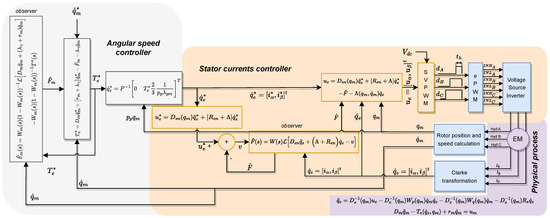
Figure 2. Illustration of the control strategy.

4. Hardware Setup

• Overview
  The test bench’s primary components are highlighted in Figure 3 and are self-explanatory. The main components are (a) a DSP dual-core 200 MHz–800 MIPS development board; (b) a three-phase gallium nitride (GaN) inverter with a nominal power of 480 W; (c) a 5 V to 3.3 V voltage translator for Hall sensor connection to the DSP; (d) an electric machine with a nominal power of 350 W; (e) a CAN interface; and (f) open- and short-circuit stator phase switches. Figure 4 highlights the main electrical connections. Via a Serial Communication Interface (SCI) over USB, the control board interfaces with the acquisition GUI shown in Figure 5. The communication is full-duplex established through the receiver (SCI_RX) and transmitter (SCI_TX) ports. This communication channel is used for parameter tuning the transmission of set points, and for the measurement of the controlled variables. The CAN adapter, based on an integrated circuit ADM3053, is used for debugging. The JTAG connector is used for writing the binary HEX file to the DSPs program and data memory modules. To eliminate unwanted power ripples caused by the fast switching of the Enhanced Pulse Width Modulation (ePWM) block and possibly slower switching or a reaction of the power supply, a linear DC supply was employed instead of a switching DC supply.
• GaN inverter specifications
  The three-phase GaN inverter has an input voltage range of 12 V to 60 V and a peak output current of 7 ARMS or 10A. It was tested up to 100 kHz PWM (by manufacturer). The GaN power stage features low switching losses, allowing for high PWM switching frequencies and a peak efficiency of up to 98.5% at 100 kHz PWM. Switch node voltage overshoot and undershoot are at low levels with a low 12.5 ns deadband. The inverter minimizes phase voltage ringing while also reducing phase voltage distortions and electromagnetic interfaces. The LMG5200 gate driver and 3.3 V band-gap reference are powered by a 5 V rail, while the INA240 current sense amplifiers and temperature switch are powered by a 3.3 V rail [24].
• DSP-Inverter data acquisition
  The use of peripherals on the DSP side is seen in Figure 4. Data from the hall sensor are collected from general input-output ($GPIO$) ports. The three-phase terminal voltages obtained from the ADC inputs are denoted as $VSENx$, while the ADC current measurements are provided by a shunt resistor amplified by linear amplifiers. The electrical machine connection to the voltage source inverter is denoted by $MOTx$. The high-side and low-side connections to the gate driver are denoted by $INHx$ and $INLx$, respectively. $ENGATE$ is the gate driver enable signal, and $PVDD$ is a DC voltage-proportional analog signal. The Enhanced Capture and Compare (ECAP) ports are used to determine the time interval between a rising and lower edge of the Hall signals, as a redundant speed measurement method.

Figure 3. (a) DSP control board; (b) Three-phase GaN inverter; (c) Hall voltage level translator; (d) Electrical machine; (e) CAN interface; (f) Open- and short-circuit stator phase switches.

Figure 4. Illustration of the electrical connections between DSP and GAN inverter.

Figure 5. View of the real-time SCI interface GUI implemented in Simulink.

Figure 5 is an image of the GUI used for transmitting and receiving data through the SCI interface. Primarily, the transmitted data are set points and controller parameters, and the received data are the controlled variable. The GUI implements five operating modes for the electrical machine, of which three are used in experiments: $inverterOFF$, $currentcontrol$, and $speedcontrol$. The fields $param1\dots param4$ are used for controller tuning at run time (i.e., dissipating factors and observer coefficients). The currents and speed references are set through the GUI, which further transmits the data via a USB-to-SCI converter to the DSP receiving buffer. The inverter switch seen in Figure 5 is implemented as a measure of protection to prevent damage to the system during tests. The communication speed over SCI was configured at a maximum of 5 Mb/s as can be seen in the GUI image. The block CalcTBPRD calculates the value of the register timer base period (TBPRD) of the ePWM module, setting the frequency of the PWM. The blocks asynchronous rate transitions are buffers used to synchronise data generated and consumed at different recurrences.

The control software was implemented in a model-based development (MBD) paradigm. We developed a Simulink model that can execute model-in-the-loop (MIL) and software-in-the-loop (SIL) simulations and can generate C code using the embedded coder feature in Matlab. In MIL mode, we simulated the control algorithm and the process model with 64-bit floating point data types. In SIL mode, the simulation was performed with a 32-bit fixed-point representation, while the generated code uses a 32-bit fixed-point data type with varying Q-format depending on the range of each signal or variable. The generated C code was compiled and linked and then loaded into the DSP flash memory by the JTAG programmer. Figure 6 depicts the Simulink model with the main tasks and their recurrences:

• The rotor speed controller task;
• The ADC interrupt-based input data acquisition task (i.e., phase currents, phase voltages);
• The rotor and position speed calculation task (determines the electrical angle and rotor speed from the three-phase Hall sensors);
• The current controller task;
• The SCI data transmitter task;
• The SCI data receiver task.

When generating code, the process model is not considered by the code generator; therefore, the same Simulink file was used for both simulations and code generation. Table 1 and Table 2 provide the control and motor parameters.

Table 1. Control parameters.

Parameter	Value
Current ($\alpha$) dissipating factor (${\lambda }_{\alpha }$)	9 [$\mathsf{\Omega }$]
Current ($\beta$) dissipating factor (${\lambda }_{\beta }$)	9 [$\mathsf{\Omega }$]
$W\left(s\right)$ numerator coefficients ($k_{\alpha }$, $k_{\beta }$)	1000 [-]
$W\left(s\right)$ denominator coefficients ($q_{\alpha }$, $q_{\beta }$)	1000 [-]
Outer loop dissipating factor (${\lambda }_{\gamma }$)	0.01
$W_m\left(s\right)$ numerator coefficient ($k_{\gamma }$)	5
$W_m\left(s\right)$ denominator coefficient ($q_{\gamma }$)	5
Recurrence time of angle processing chain	0.0002 [s]
Recurrence time of current control loop	0.0001 [s]
Recurrence time of angular speed control loop	0.0005 [s]
ADC acquisition time	Interrupt-based (end-of-conversion) ∼ 50 [uS])
Inverter PWM frequency ($F_{PWM}$)	20 [kHz]

Table 2. IWSM parameters.

Parameter	Value
Number of poles ($p_p$)	15 [-]
Nominal stator resistance ($r_s$)	0.5 [$\mathsf{\Omega }$]
Nominal stator inductance ($L_d,L_q$)	5 × 10${}^{-4}$ [H]
Permanent magnet flux (${\lambda }_{pm}$)	0.012 [$Wb$]
Torque constant ($K_{tn}$)	0.285 [$Nm/A_{rms}$]
Rotor inertia ($D_m$)	4.4 × 10${}^{-3}$ [kg m${}^2$]
Rotor viscous damping ($r_m$)	0.015 [Nm/rad/s]
Nominal power ($P_n$)	350 [W]
Nominal voltage ($V_n$)	36 [V]

Figure 6. View of the Simulink model.

5. Experimental Results

5.1. Test Bench Results

We present below the experimental result of the fixed-point implementation of the control algorithm on DSP TMS320F28379D [25]. We considered two test scenarios. In the first test case presented in Figure 7, we evaluated the control performance of the inner loop (i.e., current control). We set up the experimental test bench in current control mode through the main panel (Figure 5). We transmitted the current set point through the communication interface. The communication delay is noticeable on the data bus; however, the control loop is executed on the DSP side, so there is no impact on the control performance. The communication delay can be as high as 300 ms on two-way transmission. Experiments have shown response times between 1 and 2 ms. The results are good, since the free response time, which is 4–5 times the ratio between inductance and resistance at standstill, is approximately 5 ms. The overshoot can be seen on the right side of Figure 7 and is usually below $2.5\%$. The current ripple is caused by the space vector modulator.

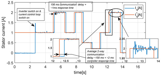
Figure 7. Stator quadrature current (experimental test I).

In the test scenario depicted in Figure 8 and Figure 9, we tested the outer control loop with a reference speed step. The ripple seen in the figures is not due to the control misbehaviour, but due to the low resolution of the speed-sensing elements—constituted out of three Hall sensors positioned at 120 electrical degrees apart. In fact, we can see that the control behaves very well under this circumstance The measured response and steady-state time are 90 ms with an overshoot of no more than $8\%$. Figure 9 shows the stator current under the same test scenario. The communication latency on the SCI port varies between 100 and 500 ms; however, we only transmitted set-point values and controller calibrations. The cascaded control loops are executed in real time on the processor side and are not affected by the high latency of the data port.

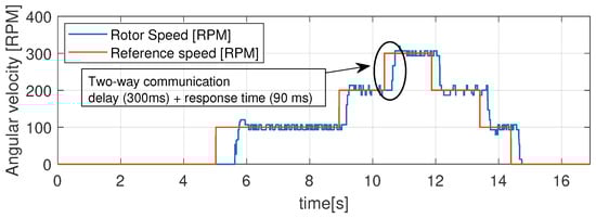
Figure 8. Rotor speed (experimental test II).

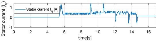
Figure 9. Stator quadrature current (experimental test II).

The response time performance of the control system can be judged better if we consider the forced response of the current loop. Therefore, in Figure 10, we input a current step to the inner loop to time the forced response. In approximately 700 ms, the wheel accelerates from 0 to 420 RPM. The acceleration is relatively slow due to the higher inertia of the wheel. Therefore, the response time of 90 ms depicted in Figure 8 can be considered a good result.

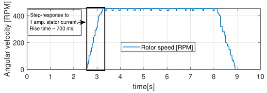
Figure 10. Rotor speed (experimental test III).

In the test case represented in Figure 11 and Figure 12, we provide a sequence of negative and positive speed steps as set points. We evaluated the transient time and the overshoot. As expected, when switching from negative to positive speed set points, the wheel reaches zero speed and the wheel inertia effect is more obvious. The overall response time is slower, 180 ms, and the transient time is 390 ms. Figure 12 shows the stator current under the same test scenario.

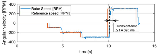
Figure 11. Rotor speed (experimental test IV).

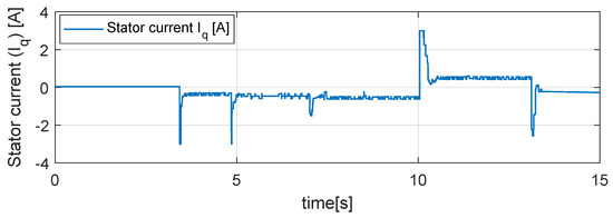
Figure 12. Stator quadrature current (experimental test IV).

5.2. Numerical Results

Below are the numerical results in SIL mode obtained based on fixed-point operations according to the DSP under consideration. In the test case represented in Figure 13, we simulated the ramp response of the control system under a series of load torque steps. The observed response time is 200 ms, the transient time is 250 ms, the steady-state error is below $0.1\%$, which can be caused solely by the fixed-point representation. Generally, the tracking of the ramp reference is good, and the overshoot is below $2\%$.

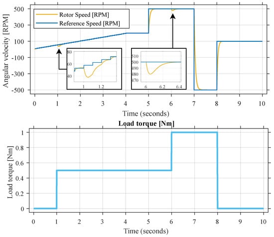
Figure 13. Rotor speed and load torque.

In the scenarios depicted in Figure 14, the control system was tested with a sequence of positive and negative speed steps under a succession of load torque steps. The observed response time is 200 ms, while the transient time is below 250 ms. The steady-state error is below $0.1\%$. The three-phase currents are recorded; the duty cycles as seen in Subfigure (d) include the third harmonic of the space vector modulator. Generally, the control performances are good, and the behavior is similar to that seen on the test bench.

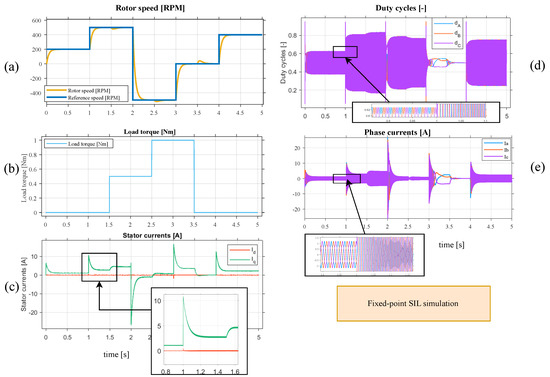
Figure 14. Software-in-the-loop simulation of the speed controller: (a) rotor speed [RPM]; (b) load torque [Nm] (c) stator currents [A]; (d) three-phase duty cycles; (e) three-phase currents [A].

In the test scenarios figured in Figure 15, we evaluated solely the current loop by providing a series of current steps. The current ripple seen in Subfigure (a) is due to the space vector modulator and can be reduced by reducing the commutation time; however, this can lead to an increase in power losses on the inverter switches. The problem of power loss is partially resolved by using GaN inverters (i.e., faster transient times between saturation and cut-off), such as the one that equips the test bench presented above. In practice, a current ripple like the one simulated in this test case, of approximately 0.3 A, is acceptable. The response time of the controller is $1.1$ ms, similar to the the test bench experiment.

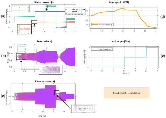
Figure 15. Software-in-the-loop simulation of the currents controller: (a) stator currents [A]; (b) three-phase duty cycles; (c) three-phase currents [A]; (d) rotor speed [RPM]; (e) load torque [Nm].

In the test cases represented in Figure 16 we evaluated the response of the current loop under varying electrical resistances. We analyzed a scenario in which the stator’s phase resistance fluctuates with a high gradient as seen in Figure 16c. This scenario would be possible in a failure event; otherwise, the phase resistance deviation is slower and caused by variations in temperature in the winding of the electrical machine. However, this scenario highlights the robust behaviour of the controller. At the time $t=1.5$ s, a sudden variation in resistance causes a higher voltage drop across the phase resistance, which in turn reduces the phase current. At the output of the passive observer, the resulting higher voltage was estimated and we computed the feed forward command applied to the process’s input. The control performances were compared against a conventional PBC controller and PI for reference. The PI is tuned by the Ziegler–Nichols method, but we adjusted the obtained parameters manually to fine tune the control performance. It is worth mentioning that the controlled system is non-linear and coupled, therefore the cross coupling of the axis has a strong impact on the PI control performance; hence, the transient time is higher. In the case of the conventional PBC, the dissipating function used in the computation of the reference voltage deviates from the nominal plant, causing a deviation in the steady-state current. Generally, the algorithm improves the behaviour of the control system to varying parameters [8,23]. In this circumstance, the overshoot of the proposed controller was 6.5%, the transient time was 1.2 ms, and the steady-state error was 0.5%. For the conventional PBC, the following performance indicators were obtained: 6.6% overshoot, greater than 5 ms transient time, and 0.4% steady-state error, while the PI controller resulted in 9% overshoot, greater than 5 ms transient time, and 0.4% steady-state error. The steady-state inaccuracy is a cumulative effect of the emulation of the PWM modulator and the implementation of the fixed-point in the SIL environment.

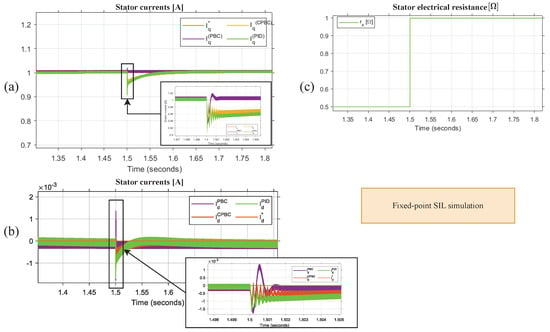
Figure 16. Comparison of software-in-the-loop simulation of currents controller under variation of phase resistance (conventional PBC, PBC, PID): (a) quadrature current [A]; (b) direct axis current [A]; (c) stator electrical resistance [$\mathsf{\Omega }$].

6. Discussion

The theoretical results are supported by simulation and experimental data, which demonstrate the effectiveness of the method. We arrive at the conditions for strict passivity in terms of the inequality constraints of the observer and controller parameters. Hence, if it is known in advance that the system to be controlled is passive, the system’s passivity can be increased to strict passivity to assure robust behaviour if the inequality constraints are preserved. In the conventional PBC, the additionally injected dissipation does not ensure null steady-state error, nor the imposed storage function, even though the stability is guaranteed by the storage function of the interconnected system. To reduce steady-state errors, we introduced the feedforward command computed from the output of the observer, and we provided the constraints of the observer and controller parameters so that the closed-loop system preserved the stability and remained farther from the instability point on the left-half plane. Generally, the control performances are improved, especially the transient time, which is reduced by more than 3–4 ms, as in the case of varying phase resistance scenarios, compared to conventional PBC and PI. The issues on the practical side relate to the lack of precision of the position detection system, which uses as input the integrated three-phase square-wave Hall sensors. The precision could be improved with linear Hall sensors. Therefore, the computed angle and speed are marginal; however, the control algorithm can generally cope with the uncertainty of the position and speed signals. We conclude that the paper brings a modest but important contribution to conventional PBC control by discussing the conditions for the passivity of the controller–observer control system and by providing an example of implementation in MBD methodology on a fixed-point DSP.

From the theoretical and practical sides, the following points could be addressed as a continuation of this study:

• The increase in the commutation frequency of the GaN inverter, but keeping the focus on balancing the torque ripple vs. power losses;
• In terms of observer design and voltage compensation terms, the presented control scheme has some similarities with the model-free controller, thus a comparison between the two should be carried out;
• The derivation of the passivity constraints for higher-order observers;
• A comparison between floating-point and fixed-point numerical implementation for the controlled and control variables, and possibly fine tuning the fixed-point’s Q-number to increase numerical precision.

References

- Xiaojuan, Y.; Jinglin, L. A novel sliding mode control for BLDC motor network control system. In Proceedings of the 2010 3rd International Conference on Advanced Computer Theory and Engineering(ICACTE), Chengdu, China, 20–22 August 2010; Volume 2, pp. 289–293. [Google Scholar] [CrossRef]
- Melkote, H.; Khorrami, F. Nonlinear adaptive control of direct-drive brushless DC motors and applications to robotic manipulators. IEEE/ASME Trans. Mechatron. 1999, 4, 71–81. [Google Scholar] [CrossRef]
- Krishnan, P.H.; Arjun, M. Control of BLDC motor based on adaptive fuzzy logic PID controller. In Proceedings of the 2014 International Conference on Green Computing Communication and Electrical Engineering (ICGCCEE), Coimbatore, India, 6–8 March 2014; pp. 1–5. [Google Scholar] [CrossRef]
- Arifiyan, D.; Riyadi, S. Hardware Implementation of Sensorless BLDC Motor Control To Expand Speed Range. In Proceedings of the 2019 International Seminar on Application for Technology of Information and Communication (iSemantic), Semarang, Indonesia, 21–22 September 2019; pp. 476–481. [Google Scholar] [CrossRef]
- Wen, H.; Yin, J. A Duty Cycle Based Finite-Set Model Predictive Direct Power Control for BLDC Motor Drives. In Proceedings of the IECON 2020 The 46th Annual Conference of the IEEE Industrial Electronics Society, Singapore, 18–21 October 2020; pp. 821–825. [Google Scholar] [CrossRef]
- Koiwa, K.; Kuribayashi, T.; Zanma, T.; Liu, K.; Wakaiki, M. Optimal current control for PMSM considering inverter output voltage limit: Model predictive control and pulse-width modulation. IET Electr. Power Appl. 2019, 13, 2044–2051. [Google Scholar] [CrossRef]
- de la Guerra, A.; Alvarez-Icaza, L. Robust Control of the Brushless DC Motor with Variable Torque Load for Automotive Applications. Electr. Power Components Syst. 2020, 48, 117–127. [Google Scholar] [CrossRef]
- Mocanu, R.; Onea, A. Robust Control of Permanent Magnet Synchronous Machine Based on Passivity Theory. Asian J. Control 2018, 20, 2034–2041. [Google Scholar] [CrossRef]
- Luo, Y.; Liu, C. A Flux Constrained Predictive Control for a Six-Phase PMSM Motor with Lower Complexity. IEEE Trans. Ind. Electron. 2019, 66, 5081–5093. [Google Scholar] [CrossRef]
- Raff, T.; Ebenbauer, C.; Allgöwer, F. Nonlinear Model Predictive Control: A Passivity-Based Approach; Springer: Berlin/Heidelberg, Germany, 2007; Volume 358, pp. 151–162. [Google Scholar] [CrossRef]
- Chen, H.; Scherer, C.W. Moving horizon H8 control with performance adaptation for constrained linear systems. Automatica 2006, 42, 1033–1040. [Google Scholar] [CrossRef]
- Tran, T.; Ha, Q. Networked control systems with accumulative quadratic constraint. Electron. Lett. 2011, 47, 108–110. [Google Scholar] [CrossRef]
- Tippett, M.J.; Bao, J. Distributed model predictive control based on dissipativity. AIChE J. 2013, 59, 787–804. [Google Scholar] [CrossRef]
- Achour, A.Y.; Mendil, B. Passivity based voltage controller-observer design with unknown load disturbance for Permanent Magnet Synchronous Motor. In Proceedings of the 2014 IEEE 23rd International Symposium on Industrial Electronics (ISIE), Istanbul, Turkey, 1–4 June 2014; pp. 201–206. [Google Scholar]
- Tao, L.; Jiuhe, W.; Yi, T.; Lei, W. A new nonlinear control stragety for PMSM. In Proceedings of the 2010 International Conference On Computer Design and Applications, Qinhuangdao, China, 25–27 June 2010; Volume 3, pp. 1152–3755. [Google Scholar]
- Riffo, S.; Gil-González, W.; Montoya, O.D.; Restrepo, C.; Muñoz, J. Adaptive Sensorless PI+ Passivity-Based Control of a Boost Converter Supplying an Unknown CPL. Mathematics 2022, 10, 4321. [Google Scholar] [CrossRef]
- Beltrán, C.A.; Diaz-Saldierna, L.H.; Langarica-Cordoba, D.; Martinez-Rodriguez, P.R. Passivity-Based Control for Output Voltage Regulation in a Fuel Cell/Boost Converter System. Micromachines 2023, 14, 187. [Google Scholar] [CrossRef] [PubMed]
- Liu, Z.; Du, J.; Stimming, U.; Wang, Y. Adaptive passivity-based control for speed regulation of permanent magnet synchronous motor. In Proceedings of the 2014 9th IEEE Conference on Industrial Electronics and Applications, Hangzhou, China, 9–11 June 2014; pp. 645–649. [Google Scholar]
- Belabbes, B.; Lousdad, A.; Meroufel, A.; Larbaoui, A. Simulation and modelling of passivity based control of PMSM under controlled voltage. J. Electr. Eng. 2013, 64, 298–304. [Google Scholar] [CrossRef]
- Cheng, Z.; Jiao, L. Hamiltonian Modeling and Passivity-based Control of Permanent Magnet Linear Synchronous Motor. J. Comput. 2013, 8, 501–508. [Google Scholar] [CrossRef]
- Bas, O.Y.; Stankovic, A.M.; Tadmor, G. Passivity based sensorless control of a smooth rotor permanent magnet synchronous motor. In Proceedings of the 36th IEEE Conference on Decision and Control, San Diego, CA, USA, 12 December 1997; Volume 1, pp. 239–244. [Google Scholar]
- Vanier, J.; Tomescu, C. Universe Dynamics: The Least Action Principle and Lagrange’s Equations; CRC Press: Boca Raton, FL, USA, 2019. [Google Scholar]
- Ortega, R.; Perez, J.A.L.; Nicklasson, P.J.; Sira-Ramirez, H.J. Passivity-Based Control of Euler-Lagrange Systems: Mechanical, Electrical and Electromechanical Applications; Springer Science & Business Media: Berlin/Heidelberg, Germany, 2013. [Google Scholar]
- 48-V, 10-A, High-Frequency PWM, 3-Phase GaN Inverter Reference Design for High-Speed Motor Drives; Texas Instruments: Dallas, TX, USA, 2017.
- TMS320F2837xD Dual-Core Microcontrollers: Technical Reference Manual; Texas Instruments: Dallas, TX, USA, 2019.
Disclaimer/Publisher’s Note: The statements, opinions and data contained in all publications are solely those of the individual author(s) and contributor(s) and not of MDPI and/or the editor(s). MDPI and/or the editor(s) disclaim responsibility for any injury to people or property resulting from any ideas, methods, instructions or products referred to in the content. |
© 2023 by the authors. Licensee MDPI, Basel, Switzerland. This article is an open access article distributed under the terms and conditions of the Creative Commons Attribution (CC BY) license (https://creativecommons.org/licenses/by/4.0/).