Deep Learning Nonhomogeneous Elliptic Interface Problems by Soft Constraint Physics-Informed Neural Networks

Abstract

It is a great challenge to solve nonhomogeneous elliptic interface problems, because the interface divides the computational domain into two disjoint parts, and the solution may change dramatically across the interface. A soft constraint physics-informed neural network with dual neural networks is proposed, which is composed of two separate neural networks for each subdomain, which are coupled by the connecting conditions on the interface. It is beneficial to capture the singularity of the solution across the interface. We formulate the PDEs, boundary conditions, and jump conditions on the interface into the loss function by means of the physics-informed neural network (PINN), and the different terms in the loss function are balanced by optimized penalty weights. To enhance computing efficiency for increasingly difficult issues, adaptive activation functions and the adaptive sampled method are used, which may be improved to produce the optimal network performance, as the topology of the loss function involved in the optimization process changes dynamically. Lastly, we present many numerical experiments, in both 2D and 3D, to demonstrate the proposed method’s flexibility, efficacy, and accuracy in tackling nonhomogeneous interface issues.

1. Introduction

Elliptic interface problems with discontinuous coefficients and singular sources are found in many applications, such as incompressible two-phase flow [1,2], computational electro-magnetics [3], heat conduction between materials of different heat capacity and conductivity [4,5,6], thermal convection in a Forchheimer–Brinkman model [7,8], etc. The solution of elliptic interface problems with discontinuous coefficients has low global regularity and usually belongs to $H^1\left(\mathsf{\Omega }\right)$ if the jump conditions are homogeneous. When the jump conditions are nonhomogeneous, the solutions to the elliptic interface problems are often discontinuous [9]. It is a difficult job to construct an efficient numerical method for such problems. In the past decades, various numerical methods have been provided to solve these kinds of problems. According to the geometric relationship between the computational grid and the material interface, the numerical method can be generally divided into two categories: (1) The interface-fitted methods [10,11,12,13,14]. In this kind of method the computational mesh fits the interface, which means that an element of the underlying mesh is required to intersect with the interface only through its edges. This approach is beneficial for the numerical scheme to reach optimal convergence. Material interactions in real-world applications can be geometrically complex and very heterogeneous. Geometric singularities, such as sharp edges, cusps, and tips, may be encountered in some extreme circumstances with nonsmooth surfaces or interfaces with Lipschitz continuity. Yet, creating high-quality meshes for some exotically complicated geometries may be challenging and time-consuming. Such a challenge drives the development of numerical algorithms that employ structured meshes and allow the interface to cut through elements. (2) The interface-unfitted method [15,16,17,18,19,20]. By allowing the interface to cut computational elements, the immersed interface approach lessens the effort of creating meshes for complicated domains and interface geometry. Specific interface techniques are required to manage interface jump conditions, which are essential for the well-posedness of the interface problem. The convergence order in the $L_{\infty }$ norm oscillates while using the interface immersed numerical approach, and the point-by-point error across the interface elements is often large.

To secure accuracy near the interface, the jump conditions on the interface have to be incorporated into the numerical discretization in a certain manner, and some special treatment needs to be introduced on the elements through which the interface passes. Although both sorts of solutions have had some success in tackling interface difficulties, implementing such numerical schemes is not an easy undertaking, due to the inhomogeneous jump conditions on the interface. High dimensional interface difficulties, nonlinear interface problems, and other generic interface problems continue to provide significant hurdles to traditional numerical methods.

Deep neural networks (DNNs) have recently received a lot of interest in the field of scientific machine learning (SciML) and have been used to build new ways of solving partial differential equations, e.g., the deep Ritz method (DRM) [21], deep Galerkin method [22] and physics-informed neural networks (PINNs) [23]. DNNs provide nonlinear approximation through the composition of hidden layers because of their universal approximation capabilities, which do not limit the approximation to linear spaces. In SciML, PINN has become one of the most prominent deep learning approaches. While the differential operators in the governing PDEs are approximated by automated differentiation, PINNs provide a mesh-free approach. Such techniques have also been applied in solving different types of partial differential equations (PDEs), including integro-differential equations [24], fractional PDEs [25], and stochastic PDEs [26,27]. Furthermore, PINNs have been effectively used to tackle a variety of issues in other domains, such as optics [28,29], fluid mechanics [30], systems biology [31], etc.

Several initiatives have been launched in recent years to employ neural networks to tackle interface problems, since neural network approaches are meshless and may benefit from deep learning techniques, such as automated differentiation and GPU acceleration. In particular, the use of multiple neural networks based on the domain decomposition method (DDM) have attracted increasing attention as they are more accurate and flexible in dealing with the interface and have shown remarkable success in various interface problems [32,33,34,35,36,37,38].

In [34], a deep-learning-based domain decomposition approach (DeepDDM) was introduced, which uses deep neural networks to discretize the subproblems split by domain decomposition methods (DDMs) to solve PDEs with complicated interfaces in the computational domain. Wang [35] proposed a mesh-free method based on DRM to solve interface problems with high-contrast discontinuous coefficients. He et al. [37] proposed a mesh-free method using piecewise DNN for elliptic interface problems with discontinuous solution and derivatives across the interface. In order to ensure that the solution is smooth in each subdomain, they approximate the solution using two neural networks that correspond to two distinct subdomains. In [33], it was suggested to use a conservative physics-informed neural network (cPINN) on discrete subdomains for nonlinear conservation laws. The computing domain is subdivided into discrete subdomains, with a different PINN applied in each subdomain. The conservation property of the cPINN is then attained by enforcing flux continuity in the strong form along the subdomain interfaces. A generalized space–time domain decomposition framework, named eXtended PINN (xPINN) was proposed in [32] to solve nonlinear PDEs in arbitrary complex-geometry domains. Wu et al. [38] performed a convergence analysis of neural network combined with domain decomposition technologies and gradient-enhanced strategies for solving second-order elliptic interface problems. It was demonstrated that, as the number of samples increased, the neural network sequence generated by minimizing a Lipschitz regularized loss function converged to the unique solution to the interface problem in $H_2$.

In this paper, we propose a soft constraint physics-informed neural network to solve the nonhomogeneous elliptic interface problems with discontinuous solutions and derivatives across the interface. Since the interface divides the domain into two disjoint parts, the solution may change dramatically across the interface. Instead of representing the approximate solutions on the whole domain with a single DNN structure, we employ two DNN structures to approximate the solution when the interface splits the domain into two subdomains. The solution is approximated by the PINNs, which formulate the PDEs and jump condition on the interface into the loss of the neural network. To improve the computational efficiency for more challenging problems, the adaptive activation function, as well as the adaptive sampling strategy, are employed to achieve the best performance as the network is optimized in the learning process. Lastly, we present many numerical experiments, in both 2D and 3D, to demonstrate the flexibility, efficacy, and accuracy of the proposed technique for handling interface issues.

The remainder of the paper is structured as follows. Section 2 describes the second-order elliptic interface issue and its three types of boundary conditions. The topology of neural networks with adaptive activation functions is discussed in Section 3. We present physical-informed neural networks with soft constraints in Section 4. Section 5 shows numerical data to demonstrate the efficacy of the suggested technique. Lastly, in Section 6, we draw some conclusions.

2. Problem Formulation

Let $\mathsf{\Omega }$ be a bounded domain in ${\mathcal{R}}^d,d=2,3$, with a border $\partial \mathsf{\Omega }$ and an interface $\mathsf{\Gamma }$ that separates $\mathsf{\Omega }$ into two disjoint subdomains, ${\mathsf{\Omega }}^{+}$ and ${\mathsf{\Omega }}^{-}$. The border $\partial \mathsf{\Omega }$ and the interface $\mathsf{\Gamma }$ are assumed to be Lipschitz continuous. The interface is defined by a piecewise smooth level-set function $\varphi \in \mathsf{\Omega }$, such that $\mathsf{\Gamma }=\left\{\overrightarrow{x}\right|\varphi \left(\overrightarrow{x}\right)=0,\forall \overrightarrow{x}\in \mathsf{\Omega }\}$. As such, two subdomains can be given by ${\mathsf{\Omega }}^{+}=\left\{\overrightarrow{x}\right|\varphi \left(\overrightarrow{x}\right)\ge 0,\forall \overrightarrow{x}\in \mathsf{\Omega }\}$ and ${\mathsf{\Omega }}^{-}=\left\{\overrightarrow{x}\right|\varphi \left(\overrightarrow{x}\right)<0,\forall \overrightarrow{x}\in \mathsf{\Omega }\}$. In some practical applications, the interface may be given as an iso value of a scalar field. $\overrightarrow{n}=\frac{\nabla \varphi }{|\nabla \varphi |}$ is the outward unit normal vector of the interface. The following second-order semi-linear elliptic interface issue is taken into consideration.

$$\left\{\begin{array}{c}-\nabla ·(\kappa \nabla u)=f\left(\overrightarrow{x}\right),\overrightarrow{x}\in {\mathsf{\Omega }}^{+}\cup {\mathsf{\Omega }}^{-},\hfill \\ \left[\right[u\left]\right]=u^{+}-u^{-}=\varphi ,\overrightarrow{x}on\mathsf{\Gamma },\hfill \\ \left[\right[\overrightarrow{\kappa }\nabla u·\overrightarrow{n}\left]\right]={\kappa }^{+}{u}_n^{+}-{\kappa }^{-}{u}_n^{-}=\psi ,\overrightarrow{x}on\mathsf{\Gamma },\hfill \\ u=\left\{\begin{array}{c}{g}_d,\overrightarrow{x}\in \partial {\mathsf{\Omega }}_d,\hfill \\ \kappa \nabla u·\overrightarrow{n}=q,\overrightarrow{x}\in \partial {\mathsf{\Omega }}_q,\hfill \\ \kappa \nabla u·\overrightarrow{n}=h(u_{\infty }-u),\overrightarrow{x}\in \partial {\mathsf{\Omega }}_h.\hfill \end{array}\right.\hfill \end{array}\right.$$

(1)

where the function $f\left(\overrightarrow{x}\right)$ describes acting source, the physical meaning of which is determined by the nature of the considered processes. The boundary $\partial \mathsf{\Omega }$ has been split into partitions $\partial {\mathsf{\Omega }}_d$, $\partial {\mathsf{\Omega }}_q$, and $\partial {\mathsf{\Omega }}_h$, each of which is mutually exclusive. Here, $\partial {\mathsf{\Omega }}_d$ corresponds to the Dirichlet boundary condition for the given temperature $g_d$ and $\partial {\mathsf{\Omega }}_q$ corresponds to the Neumann boundary condition with the heat flux $q:\partial {\mathsf{\Omega }}_q\to \mathcal{R}$, and $\partial {\mathsf{\Omega }}_h$ denotes the region with Robin (convective) boundary conditions with the heat transfer coefficient $h:\partial {\mathsf{\Omega }}_h\to \mathcal{R}$, and surrounding temperature $u_{\infty }:\partial {\mathsf{\Omega }}_h\to \mathcal{R}$. $u^{+},u_n^{+},{\kappa }^{+}$ indicate their limiting value from the ${\mathsf{\Omega }}^{+}$ side of the interface, and $u^{-},u_n^{-},{\kappa }^{-}$ indicate their limiting value from the ${\mathsf{\Omega }}^{-}$ side of the interface $\mathsf{\Gamma }$. On the interface, the derivatives $u_n^{+}$ and $u_n^{-}$ are assessed along the normal direction. $\varphi \left(\overrightarrow{x}\right)$ and $\psi \left(\overrightarrow{x}\right)$ are at least $C^1$ continuous.

3. Mathematical Setup for Dual Neural Networks Structure

A feed-forward neural network of L layers and $N_k$ neurons in the kth layer $(N_0=D_i$, and $N_L=D_o$) is denoted by $\mathcal{N}:{\mathbb{R}}^{D_i}\to {\mathbb{R}}^{D_o}$. ${\mathbf{W}}^k\in {\mathbb{R}}^{N_k\times N_{k-1}}$ and ${\mathbf{b}}^k\in {\mathbb{R}}^{N_k}$ are the weight matrix and bias vector in the kth layer $(1\le k\le L)$, respectively. The input vector is denoted by $\overrightarrow{x}\in {\mathbb{R}}^{D_i}$ and the output vector at the kth layer is denoted by ${\mathcal{N}}^k\left(\overrightarrow{x}\right)$ and ${\mathcal{N}}^0\left(\overrightarrow{x}\right)=\overrightarrow{x}$. The activation function is denoted by $\mathsf{\Phi }$ and is applied layer-wise together with the scalable parameters $n{a}^k$, where n is the scaling factor. The extra parameters $a^k$ modify the slope of the activation function in each hidden layer, resulting in faster training speed. By means of the slope recovery term, the activation slopes can also influence the loss function, see [39,40] for more details. Such locally adaptable activation functions, in particular during the initial training phase, improve the network’s potential for learning. This document uses a scaling factor $n=5$ for all hidden layers and an initialization $n{a}^k=1,\dots ,k$.

The $(L-1)$-hidden layer feed-forward neural network is defined by

$${\mathcal{N}}^k={\mathbf{W}}^k\mathsf{\Phi }\left(a^{k-1}{\mathcal{N}}^{k-1}\left(\overrightarrow{x}\right)\right)+{\mathbf{b}}^k,2\le k\le L$$

(2)

and ${\mathcal{N}}^1\left(\overrightarrow{x}\right)={\mathbf{W}}^1\overrightarrow{x}+b^1$, where, on the first layer, the activation function is identity. $\mathsf{\Theta }=\{{\mathbf{W}}^k,{\mathbf{b}}^k,a^k\}\in \mathrm{V}$ is the collection of all weights, biases, and slopes and takes $\mathrm{V}$ as the parameter space.

However, unlike conventional approaches that use only a single DNN to approximate the $u\left(\overrightarrow{x}\right)$ solution over the entire $\mathsf{\Omega }$ domain, we use two DNN structures independently to estimate $u^{+}\left(\overrightarrow{x}\right)$ and $u^{-}\left(\overrightarrow{x}\right)$ on ${\mathsf{\Omega }}^{+}$ and ${\mathsf{\Omega }}^{-}$, respectively. For $\overrightarrow{x}\in {\mathsf{\Omega }}_i,i=1,2$, a dual neural network is used to approximate $u_i\left(\overrightarrow{x}\right),i=1,2$, as follows,

$$u_i\left(\overrightarrow{x}\right)\approx {\mathcal{U}}_{i,\mathcal{N}}(\overrightarrow{x},{\mathsf{\Theta }}_i)={\mathcal{N}}_i^L\circ {\mathcal{N}}_i^{L-1}\circ \dots \circ {\mathcal{N}}_i^2\circ {\mathcal{N}}_i^1\left(\overrightarrow{x}\right),i=1,2,$$

(3)

where ${\mathcal{U}}_{i,\mathcal{N}}(\overrightarrow{x},{\mathsf{\Theta }}_i)$ highlights the dependence of the neural network output ${\mathcal{U}}_{i,\mathcal{N}}\left(\overrightarrow{x}\right)$ on ${\mathsf{\Theta }}_i$. Then, the global approximation of $u\left(\overrightarrow{x}\right)$ can be defined as follows,

$$u\left(\overrightarrow{x}\right)\approx {\mathcal{U}}_{\mathcal{N}}(\overrightarrow{x},\mathsf{\Theta })=\left\{\begin{array}{c}{\mathcal{U}}_{1,\mathcal{N}}(\overrightarrow{x},\mathsf{\Theta }),if\overrightarrow{x}\in {\mathsf{\Omega }}_1,\hfill \\ {\mathcal{U}}_{2,\mathcal{N}}(\overrightarrow{x},\mathsf{\Theta }),if\overrightarrow{x}\in {\mathsf{\Omega }}_2.\hfill \end{array}\right.$$

(4)

where $\mathsf{\Theta }={\mathsf{\Theta }}_i$, if $\overrightarrow{x}\in {\mathsf{\Omega }}_i,i=1,2$. ${\mathcal{U}}_{\mathcal{N}}(\overrightarrow{x},\mathsf{\Theta })$ emphasizes the dependence of the neural network output $U_{\mathcal{N}}\left(\overrightarrow{x}\right)$ on $\mathsf{\Theta }$.

4. Physics-Informed Neural Networks with Soft Constraints

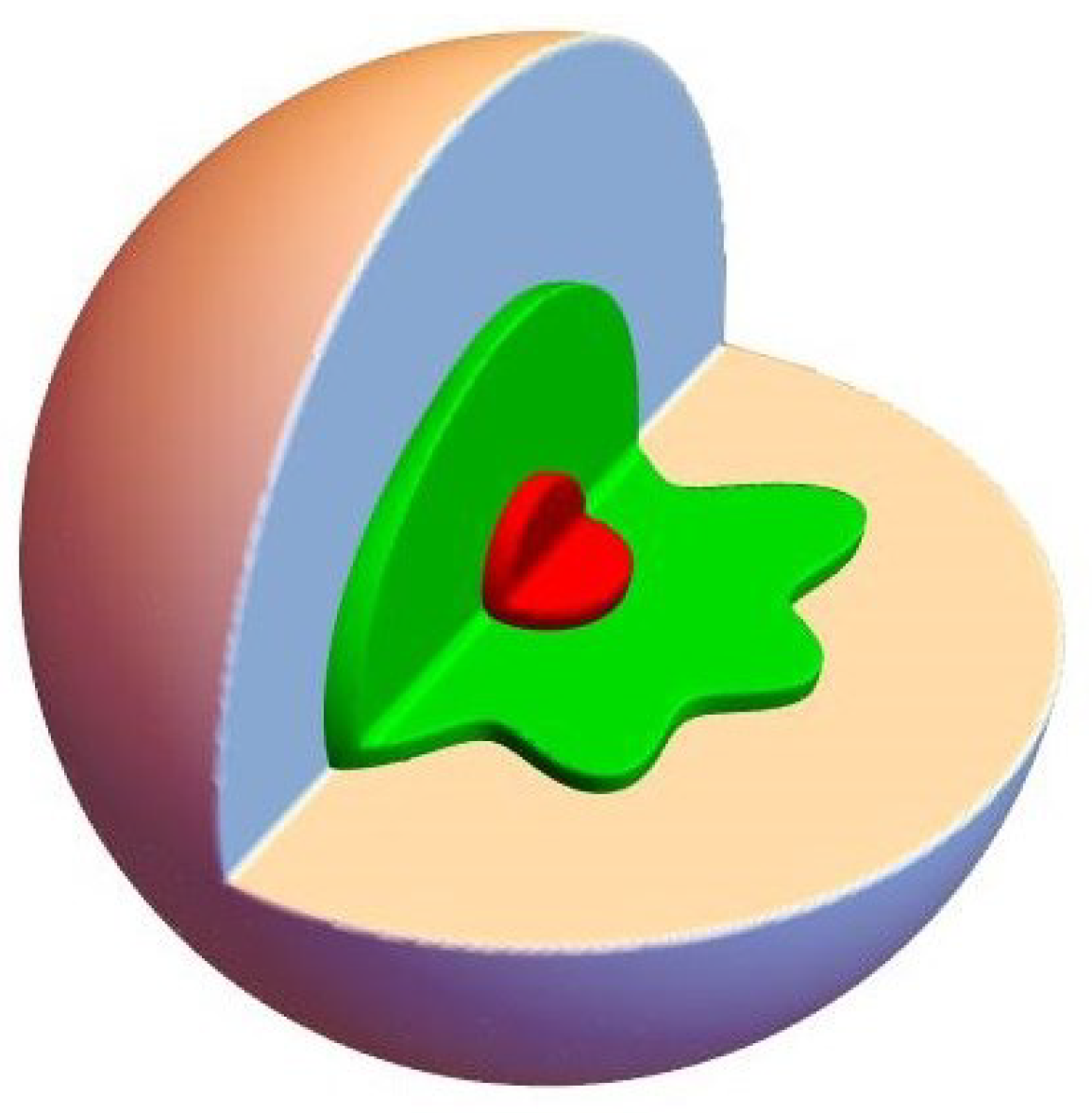
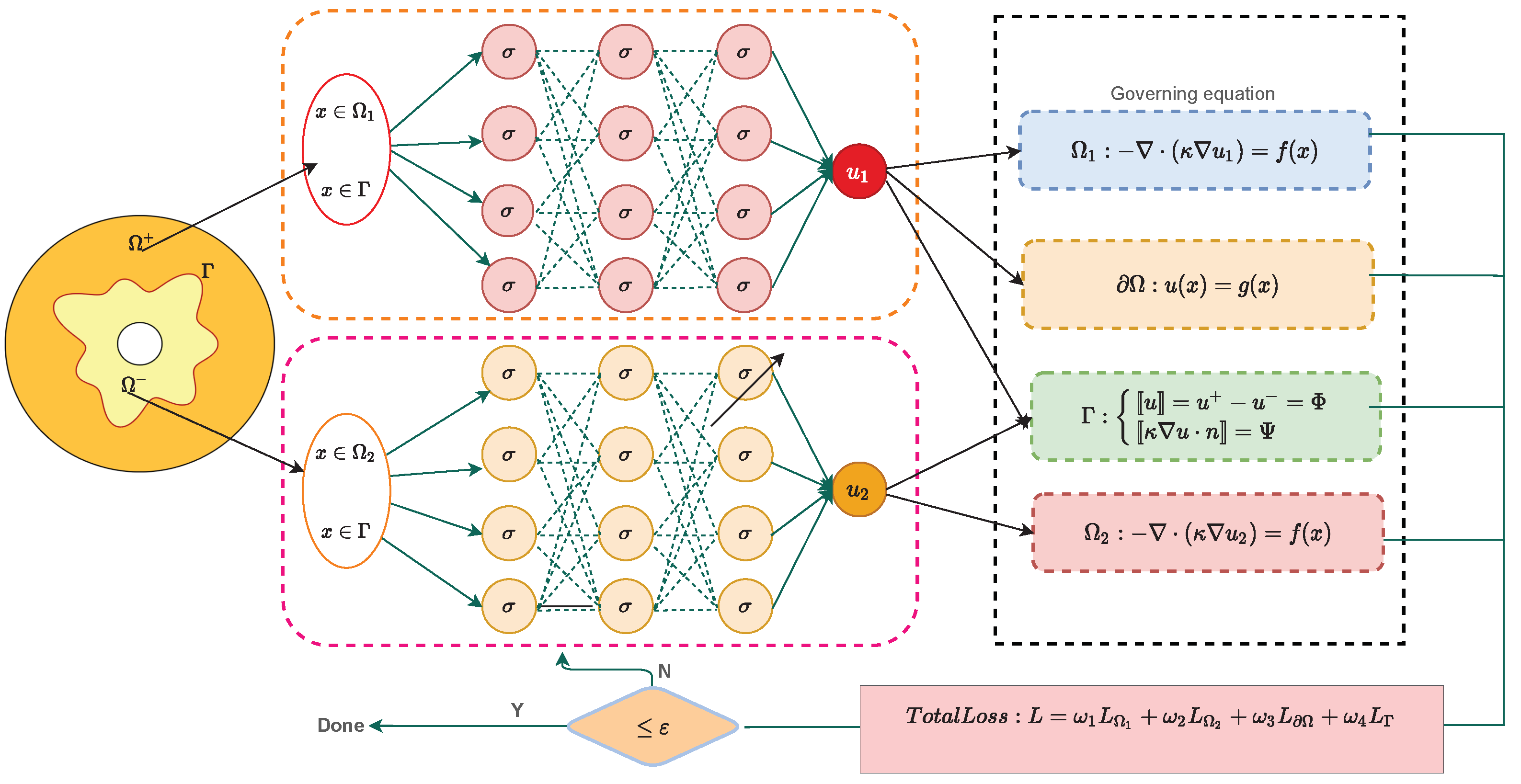
A key feature of a PINN is that it can easily turn a PDE problem into an optimization problem by combining all available information, including control equations, empirical data, and initial/boundary conditions into a loss function. The advantage of this approach is that it provides a meshless algorithm, because the differential operators in the managed PDE are approximated by an automatic discriminant. To reduce the difficulty of neural network learning, we hope that the network constructed can, as far as possible, meet the general solution of PDE, and then achieve the goal of accelerating convergence speed and improving solution accuracy. The dual neural networks structure of the approximation ${\mathcal{U}}_{\mathcal{N}}(\overrightarrow{x},\mathsf{\Theta })$ is shown in Figure 1. As we can see, these two networks were used to approximate the solution in different domains. The sampling points were classified, according to the location of the sample pickup points, and then it was determined to which separate DNN network they belonged. This method can effectively approximate the singular discontinuous solution along the material interface.

For a forward problem, we define the loss function as

$$\mathcal{L}\left(\mathsf{\Theta }\right)={\omega }_1{L}_{{\mathsf{\Omega }}_1}+{\omega }_2{L}_{{\mathsf{\Omega }}_2}+{\omega }_3{L}_{\mathsf{\Gamma }}+{\omega }_4{L}_{\partial \mathsf{\Omega }}+{\omega }_5{L}_d,$$

(5)

where $L_{{\mathsf{\Omega }}_1}$ and $L_{{\mathsf{\Omega }}_2}$ are the losses corresponding to the residuals of governing equations in subdomains ${\mathsf{\Omega }}_1$ and ${\mathsf{\Omega }}_2$, respectively. $L_{\partial \mathsf{\Omega }}$ is the loss due to the boundary condition, $L_{\mathsf{\Gamma }}$ is the loss due to the interface conditions, and $L_d$ is the loss corresponding to label data (if any).

$$\begin{array}{ccc}\hfill L_{{\mathsf{\Omega }}_1}& =& \frac{1}{N_{r1}}\sum _{i=1}^{N_{r1}}{|-\nabla ·(\kappa \nabla u_1(x_{r1}^i,\theta ))-f_1|}^2,\hfill \\ \hfill L_{{\mathsf{\Omega }}_2}& =& \frac{1}{N_{r2}}\sum _{i=1}^{N_{r1}}{|-\nabla ·(\kappa \nabla u_2(x_{r2}^i,\theta ))-f_2|}^2,\hfill \\ \hfill L_{\mathsf{\Gamma }}& =& \frac{1}{N_I}\sum _{i=1}^{N_I}|\left[\left[u^i\right]\right]{-\varphi |}^2+\sum _{i=1}^{N_I}{|\left[[\kappa \nabla u(x_{\gamma }^i,\theta )·n]\right]-\psi |}^2,\hfill \\ \hfill L_{\partial \mathsf{\Omega }}& =& \frac{1}{N_b}\sum _{i=1}^{N_b}{|u(x_b^i;\theta )-g_b^i|}^2\hfill \\ \hfill L_d& =& \frac{1}{N_d}\sum _{i=1}^{N_d}|\widehat{u}(x_d^i,\theta ){)-y_d^i|}^2,\hfill \end{array}$$

where ${\left\{{\overrightarrow{x}}_{r1}^i\right\}}_{i=1}^{N_{r1}}$ and ${\left\{{\overrightarrow{x}}_{r2}^i\right\}}_{i=1}^{N_{r2}}$ are the collocation points randomly distributed in the domain ${\mathsf{\Omega }}_1$ and ${\mathsf{\Omega }}_2$, ${\{{\overrightarrow{x}}^i,g_b^i=g\left({\overrightarrow{x}}_b^i\right)\}}_{i=1}^{N_b}$ are the boundary condition points, ${\left\{{\overrightarrow{x}}_I^i\right\}}_{i=1}^{N_{\mathsf{\Gamma }}}$ are the interface condition points, and ${\{{\overrightarrow{x}}_d^i,t_d^i\}}_{i=1}^{N_d}$ are sample data (if any). $N_{{\mathsf{\Omega }}_1}$, $N_{{\mathsf{\Omega }}_2}$, $N_{\mathsf{\Gamma }}$, $N_{\partial \mathsf{\Omega }}$, $N_d$ denote the total number of collocation points in two different regions, interface points, boundary points and labeled data, respectively. The weights ${\omega }_1$, ${\omega }_2$, ${\omega }_3$, ${\omega }_4$ and ${\omega }_5$ are the weights of residuals for two governing equations, interface conditions, boundary conditions, and labeled data. Weights in PINNs are crucial for learnability and can be set manually or auto-configured [41,42,43].

The basic idea is to train a neural network to approximate the solution of PDE by minimizing the physically-informed loss function, given the residual of the PDEs together with the interface and boundary conditions, as follows:

$${\mathsf{\Theta }}^{*}=\underset{\mathsf{\Theta }}{argmin}\mathcal{L}\left(\mathsf{\Theta }\right).$$

where ${\mathsf{\Theta }}^{*}$ is the minimizer and ${\mathcal{U}}_{\mathcal{N}}(\overrightarrow{x};{\mathsf{\Theta }}^{*})$ is the related DNN approximation.

5. Numerical Experiments

Several numerical tests for the elliptic interface problems in two and three dimensions were carried out, using the current soft constraint PINNs. Due to these intricate contact geometries, traditional numerical methods for handling such problems provide a significant challenge to the robustness of numerical schemes. Apart from numerical scheme concerns, the great computational complexity of typical numerical approaches for three-dimensional problems is a significant challenge in dealing with complex interface challenges. As a result, this section highlights the benefits and potential utility of deep learning approaches in dealing with such difficult numerical instances. The setup we use in the example below aims to demonstrate the robustness and efficacy of the suggested algorithm, even in the case of a small network architecture. By choosing the sigmoid as the activation function, we terminate the learning process when the stopping standardization $Loss\left(\mathsf{\Theta }\right)<\epsilon$ is satisfied (the $\epsilon$ tolerance was set to at least ${10}^{-5}$). Cross-validation was used in machine learning practice for validation. That is, we used the test error instead of the training error to measure the accuracy of the solution. The $L_{\infty }$ and $L_2$ norm errors are calculated by randomly selecting test points $N_{test}$ located in $\mathsf{\Omega }$ as

$$\parallel \widehat{u}{-u\parallel }_{\infty }=\underset{1\le i\le N_{test}}{max}\frac{|\widehat{u}\left({\overrightarrow{x}}^i\right)-u\left({\overrightarrow{x}}^i\right)|}{|\widehat{u}\left({\overrightarrow{x}}^i\right)|},{\parallel \widehat{u}-u\parallel }_2=\sqrt{\frac{{\sum }_{i=1}^{N_{test}}{|\widehat{u}\left({\overrightarrow{x}}^i\right)-u\left({\overrightarrow{x}}^i\right)|}^2}{{\sum }_{i=1}^{N_{test}}{\left|\widehat{u}\left({\overrightarrow{x}}^i\right)\right|}^2}},$$

(6)

where $\widehat{u}$ was the function obtained by the present PINN.

Example 1.

This example employs a sophisticated interface in the form of parameters

$$x\left(\theta \right)=(a+bcos\left(m\theta \right))sin\left(n\theta \right)cos\left(\theta \right),y\left(\theta \right)=\left(a+bcos\left(m\theta \right)\right)sin\left(n\theta \right)sin\left(\theta \right),$$

(7)

where $\theta \in [0,2\pi ]$, $a=b=0.40178$, $m=2$ and $n=6$. The coefficients ${\kappa }^{\pm }$ and the solutions $u^{\pm }$ are given as follows

$$\kappa =\left\{\begin{array}{c}\frac{2+xy}{5},(x,y)\in {\mathsf{\Omega }}^{+},\hfill \\ \frac{x^2-y^2+3}{7},(x,y)\in {\mathsf{\Omega }}^{-},\hfill \end{array}\right.u=\left\{\begin{array}{c}x+y+1,(x,y)\in {\mathsf{\Omega }}^{+},\hfill \\ sin(x+y)+cos(x+y)+1,(x,y)\in {\mathsf{\Omega }}^{-}.\hfill \end{array}\right.$$

(8)

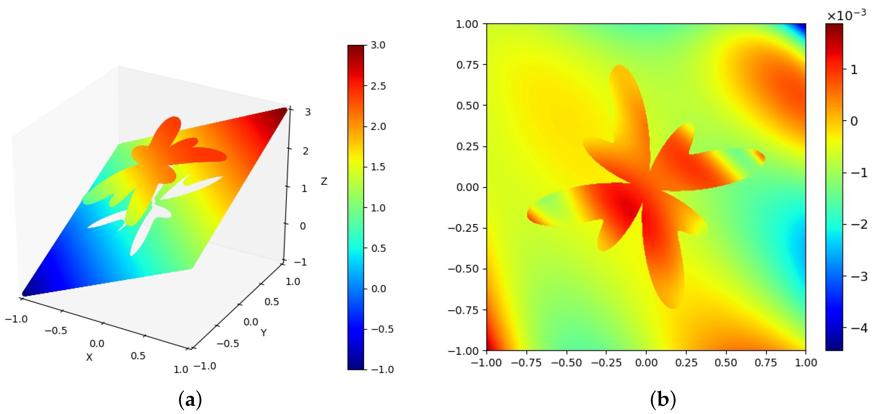
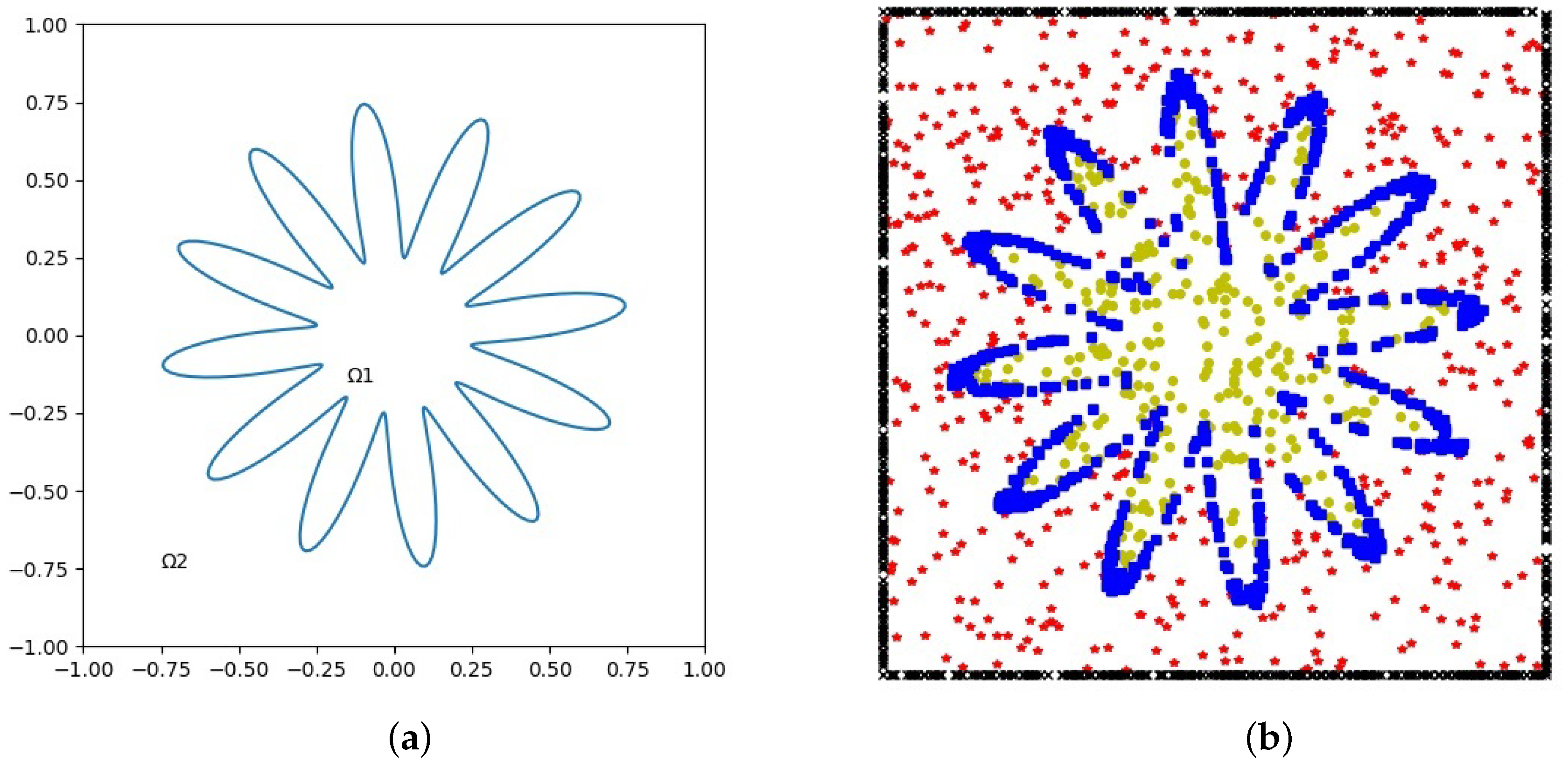
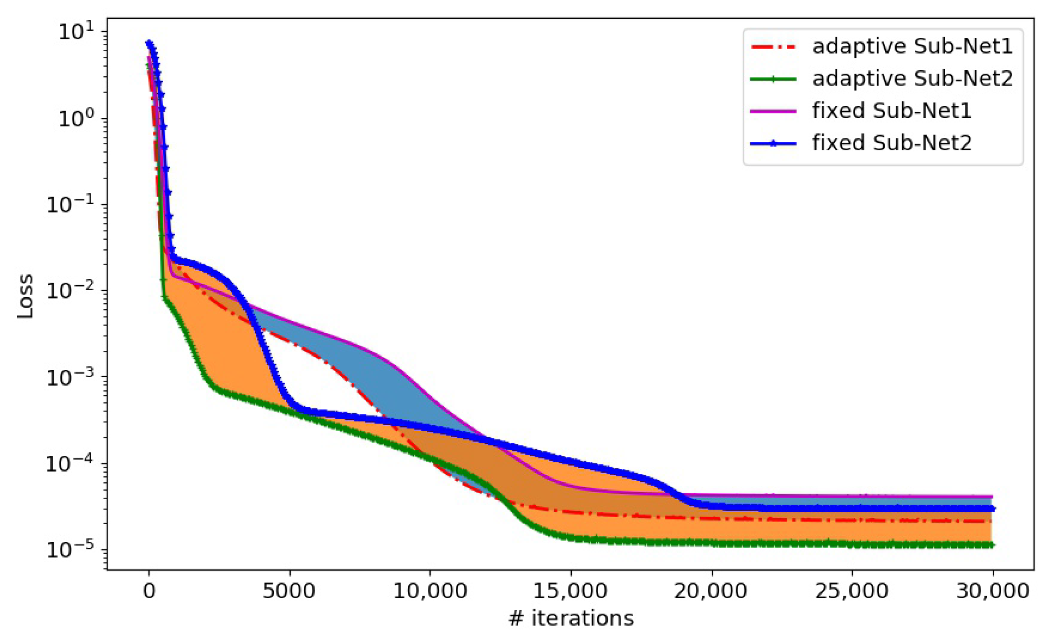
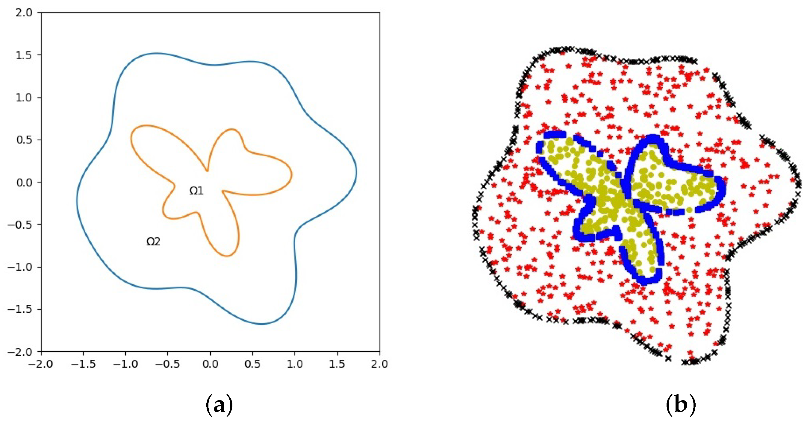
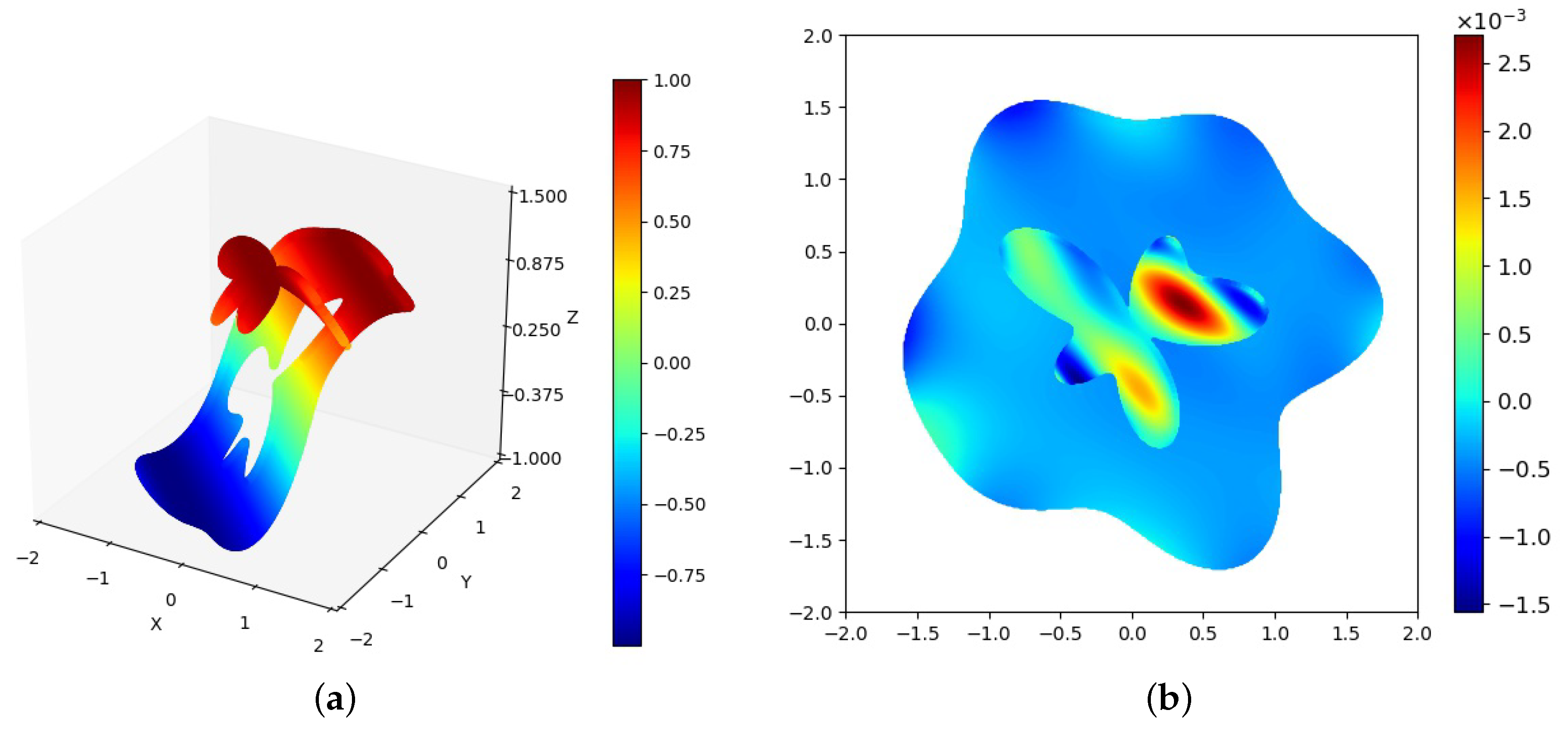
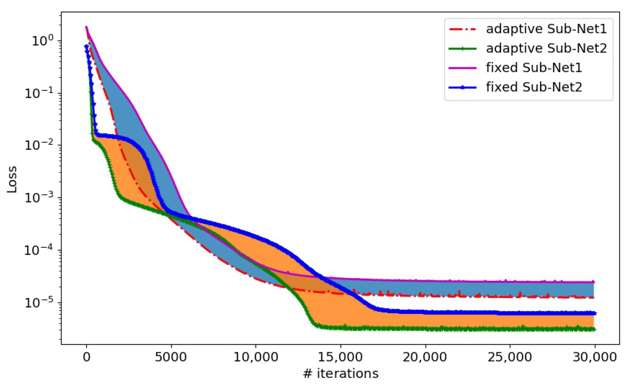
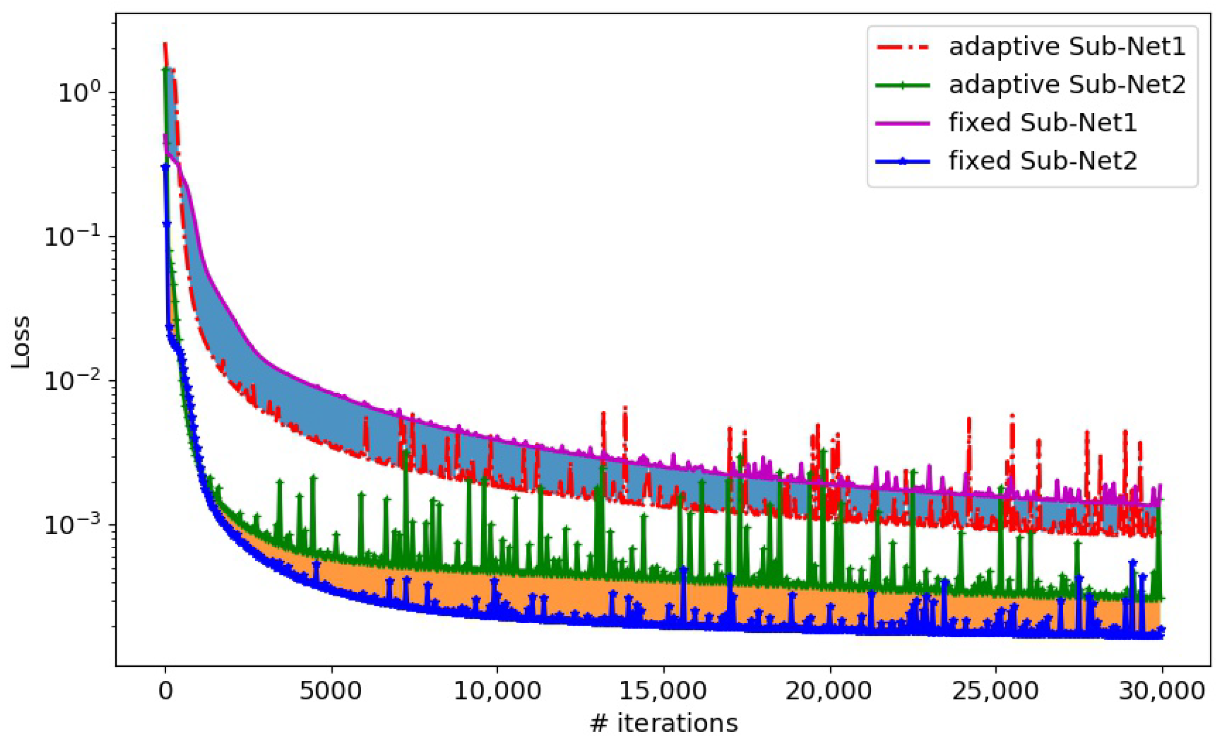
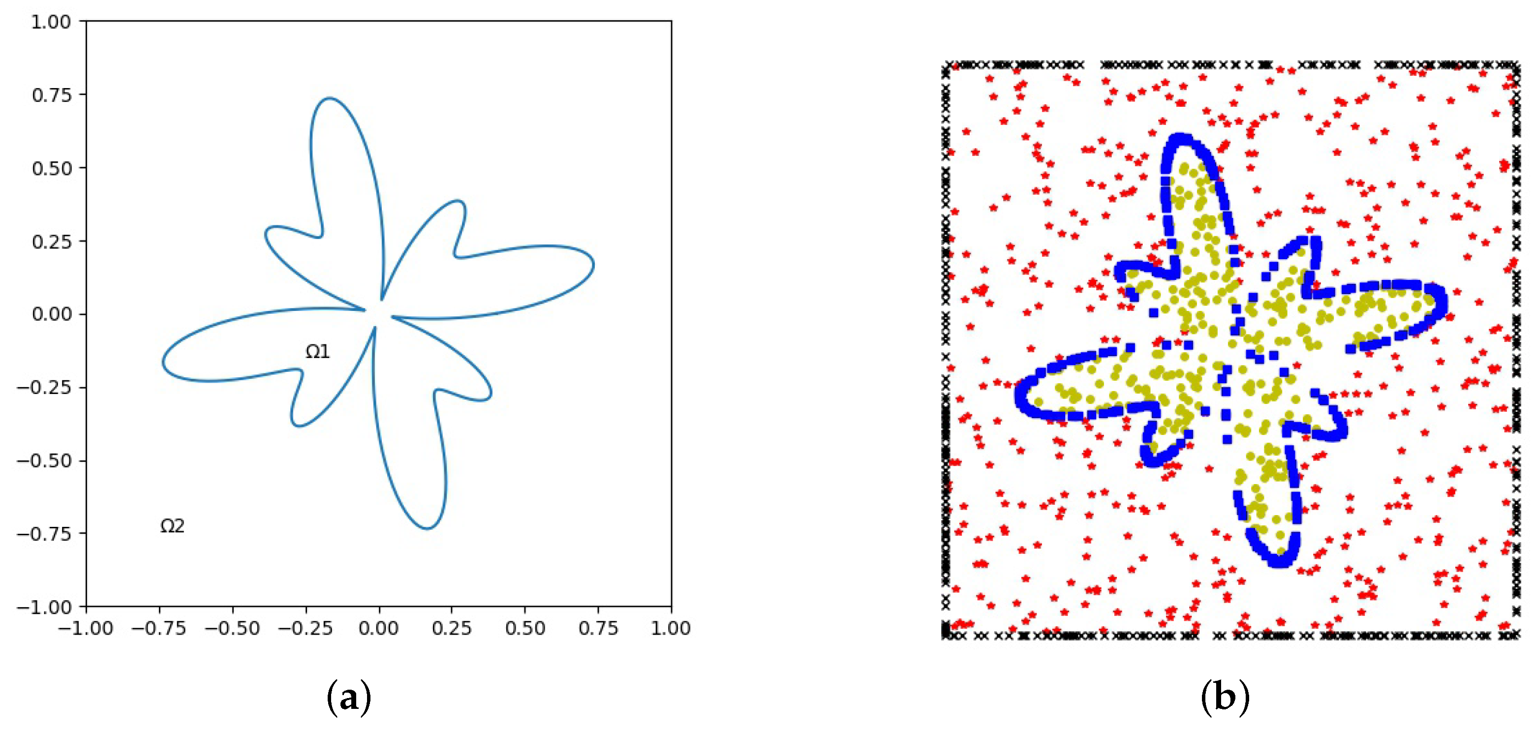
A dual neural network with 3 layers and 20 neurons in each layer was used. The geometry of interface $\mathsf{\Gamma }$ and subdomains is illustrated in Figure 2a. The uniform sampled points with $N_{r1}=500$ on the domain ${\mathsf{\Omega }}_1$, $N_{r2}=300$ on the domain ${\mathsf{\Omega }}_2$ and $N_{\mathsf{\Gamma }}=300$ on the interface $\mathsf{\Gamma }$, and $N_{\partial \mathsf{\Omega }}=800$ on the boundary $\partial \mathsf{\Omega }$, were used to calculate the numerical solution, see Figure 2b. The balance weights in the loss function were chosen as ${\omega }_1=0.00001$, ${\omega }_2=0.00001$, ${\omega }_3=0.99999$, ${\omega }_4=0.99999$. The PINN solution is shown in Figure 3a. The error between PINN and exact solutions is shown in Figure 3b. It can be seen that the presented PINN was able to approximate the solution of the interface problem, and the relative error between the numerical and the analytical solution was between $-4.0\times {10}^{-3}$ and $1.0\times {10}^{-3}$. Figure 4 presents the evolution process of the loss function with adaptive and fixed activation functions for Sub-Net1 and Sub-Net2, respectively. It is shown that the adaptive activation function was beneficial in improving the convergence speed of the loss function in the process of deep learning.

Table 1. Comparison of the errors of the adaptive and the fixed activating function strategies for different numbers of training points for Example 1.

Activation Function	${\mathit{N}}_{\mathit{\partial }\mathbf{\Omega }}$/${\mathit{N}}_{\mathit{r}1}$/${\mathit{N}}_{\mathit{r}2}$/${\mathit{N}}_{\mathbf{\Gamma }}$	${\mathit{e}}_{{\mathbf{\Omega }}_1}$	${\mathit{e}}_{{\mathbf{\Omega }}_2}$	${\mathit{e}}_{\mathbf{\Gamma }}$	${\mathit{e}}_{\mathit{\partial }\mathbf{\Omega }}$
	$200/500/300/75$	9.997 × 10${}^{-4}$	6.553 × 10${}^{-4}$	6.621 × 10${}^{-4}$	7.786 × 10${}^{-4}$
Adaptive	$400/500/300/150$	7.223 × 10${}^{-4}$	4.552 × 10${}^{-4}$	2.800 × 10${}^{-4}$	5.483 × 10${}^{-4}$
	$800/500/300/300$	4.539 × 10${}^{-4}$	3.675 × 10${}^{-4}$	3.319 × 10${}^{-4}$	5.771 × 10${}^{-4}$
	$200/500/300/75$	5.137 × 10${}^{-4}$	7.497 × 10${}^{-4}$	6.797 × 10${}^{-4}$	5.013 × 10${}^{-4}$
Fixed	$400/500/300/150$	4.997 × 10${}^{-4}$	6.513 × 10${}^{-4}$	6.628 × 10${}^{-4}$	5.186 × 10${}^{-4}$
	$800/500/300/300$	4.560 × 10${}^{-4}$	4.164 × 10${}^{-4}$	3.724 × 10${}^{-4}$	4.843 × 10${}^{-4}$

shows the relative $L_2$ errors with the different number of training points under the adaptive activation function and fixed activation function. $e_{{\mathsf{\Omega }}_1}$, $e_{{\mathsf{\Omega }}_2}$, $e_{\mathsf{\Gamma }}$ and $e_{\partial \mathsf{\Omega }}$ are the loss errors at ${\mathsf{\Omega }}^{+}$, ${\mathsf{\Omega }}^{-}$, interface $\mathsf{\Gamma }$ and boundary $\partial \mathsf{\Omega }$, respectively. It can be seen that the error decreased with increase in the number of training points on the boundary and interface, and the error by the adaptive activation function method was better than that of the fixed activation function.

Table 2. Comparison of errors in different terms with different numbers of neurons for Example 1.

Number of Neurons	${\mathit{e}}_{{\mathbf{\Omega }}_1}$	${\mathit{e}}_{{\mathbf{\Omega }}_2}$	${\mathit{e}}_{\mathbf{\Gamma }}$	${\mathit{e}}_{\mathit{\partial }\mathbf{\Omega }}$
10	1.007 × 10${}^{-3}$	3.101 × 10${}^{-4}$	3.336 × 10${}^{-4}$	5.140 × 10${}^{-4}$
20	5.397 × 10${}^{-4}$	4.652 × 10${}^{-4}$	3.488 × 10${}^{-4}$	6.003 × 10${}^{-4}$
40	2.912 × 10${}^{-4}$	1.573 × 10${}^{-4}$	1.208 × 10${}^{-4}$	1.967 × 10${}^{-4}$

presents the relative $L_2$ errors of the same training points with different numbers of neurons. In this table, we can see that the calculation accuracy increased with increase in the number of neurons, but the calculation time cost increased accordingly. Therefore, the appropriate network depth and width should be selected in order to acquire good accuracy and efficiency.

Example 2.

This example used the same interface geometric parameter equation as in Example 1. The same problem setting and analysis solution as in the previous example and the balance weight in the loss function were used. Here, $a=0.50012563$, $b=0.250012563$, $m=0$, and $n=12$. The geometry of interface Γ and subdomains is illustrated in Figure 5a. The numerical solution was calculated on the uniform sampled points with $N_{r1}=500$, $N_{r2}=300$, $N_{\mathsf{\Gamma }}=300$, and $N_{\partial \mathsf{\Omega }}=800$, see Figure 5b. The PINN solution is shown in Figure 6a. The relative error in $L_2$ norm is plotted in Figure 6. It can be seen that the present method effectively approximated the solution of the interface problem, and the range of error was between $-3\times {10}^{-3}$ to $3\times {10}^{-3}$. This example shows that, even at uniform sampling points, the present dual neural network technology could produce sufficient accurate approximation for two-dimensional elliptic problems with complex interface geometry. Figure 7 displays the evolution process of the loss function with adaptive and fixed activation functions for Sub-Net1 and Sub-Net2, respectively. It is shown that the adaptive activation function was beneficial in improving the convergence speed of the loss function in the process of deep learning.

Table 3. Comparison of errors by adaptive and fixed activation function strategies with different numbers of training points for Example 2.

Activation Function	${\mathit{N}}_{\mathit{\partial }\mathbf{\Omega }}$/${\mathit{N}}_{\mathit{r}1}$/${\mathit{N}}_{\mathit{r}2}$/${\mathit{N}}_{\mathbf{\Gamma }}$	${\mathit{e}}_{{\mathbf{\Omega }}_1}$	${\mathit{e}}_{{\mathbf{\Omega }}_2}$	${\mathit{e}}_{\mathbf{\Gamma }}$	${\mathit{e}}_{\mathit{\partial }\mathbf{\Omega }}$
	$200/500/300/75$	4.517 × 10${}^{-4}$	3.827 × 10${}^{-4}$	6.621 × 10${}^{-4}$	4.786 × 10${}^{-4}$
Adaptive	$400/500/300/150$	4.213 × 10${}^{-4}$	1.653 × 10${}^{-4}$	2.800 × 10${}^{-4}$	5.483 × 10${}^{-4}$
	$800/500/300/300$	4.167 × 10${}^{-4}$	1.719 × 10${}^{-4}$	2.409 × 10${}^{-4}$	4.691 × 10${}^{-4}$
	$200/500/300/75$	8.257 × 10${}^{-4}$	7.546 × 10${}^{-4}$	6.348 × 10${}^{-4}$	7.221 × 10${}^{-4}$
Fixed	$400/500/300/150$	6.458 × 10${}^{-4}$	6.114 × 10${}^{-4}$	6.227 × 10${}^{-4}$	7.102 × 10${}^{-4}$
	$800/500/300/300$	4.139 × 10${}^{-4}$	3.449 × 10${}^{-4}$	4.677 × 10${}^{-4}$	5.677 × 10${}^{-4}$

compares the relative $L_2$ errors in a different number of training points with adaptive and fixed activation functions, respectively. We can see that the error decreased with increase in the number of training points on the boundary and interface, and the error of the adaptive activation function method was better than that of the fixed activation function.

Table 4. Comparison of errors in different terms with different numbers of neurons for Example 2.

Number of Neurons	${\mathit{e}}_{{\mathbf{\Omega }}_1}$	${\mathit{e}}_{{\mathbf{\Omega }}_2}$	${\mathit{e}}_{\mathbf{\Gamma }}$	${\mathit{e}}_{\mathit{\partial }\mathbf{\Omega }}$
10	7.108 × 10${}^{-4}$	3.548 × 10${}^{-4}$	5.548 × 10${}^{-4}$	4.591 × 10${}^{-4}$
20	4.517 × 10${}^{-4}$	3.827 × 10${}^{-4}$	6.621 × 10${}^{-4}$	4.786 × 10${}^{-4}$
40	4.559 × 10${}^{-4}$	7.968 × 10${}^{-4}$	8.676 × 10${}^{-4}$	3.454 × 10${}^{-4}$

shows the relative $L_2$ errors of the same training points with a different number of neurons. It is shown that the calculation accuracy increased with increase of the number of neurons, but the calculation time cost increased accordingly.

Example 3.

Consider the following level set function to describe an annular region with inner and outer radii $r_{inn}=0.151$ and $r_{out}=0.911$ with an immersed star interface.

$$\varphi (x,y)=\sqrt{(x^2+y^2)}-r_0\left(1+\sum _{k=1}^3{\beta }_{k}cos\left(n_k(arctan\left(\frac{y}{x}\right)-{\theta }_k)\right)\right),$$

(9)

with parameters:

$$r_0=0.483,\left(\begin{array}{c}{n}_1\\ {\beta }_1\\ {\theta }_1\end{array}\right)=\left(\begin{array}{c}3\\ 0.3\\ 0.5\end{array}\right),\left(\begin{array}{c}{n}_2\\ {\beta }_2\\ {\theta }_2\end{array}\right)=\left(\begin{array}{c}4\\ -0.1\\ 1.8\end{array}\right),and\left(\begin{array}{c}{n}_3\\ {\beta }_3\\ {\theta }_3\end{array}\right)=\left(\begin{array}{c}7\\ 0.15\\ 0\end{array}\right).$$

(10)

The exact solution is

$$u=\left\{\begin{array}{c}\left(16{\left(\frac{y-x}{3}\right)}^5-20{\left(\frac{y-x}{3}\right)}^3\right)+5\left(\frac{y-x}{3}\right)log(x+y+3),(x,y)\in {\mathsf{\Omega }}^{+},\hfill \\ sin\left(2x\right)cos\left(2y\right),(x,y)\in {\mathsf{\Omega }}^{-}.\hfill \end{array}\right.$$

(11)

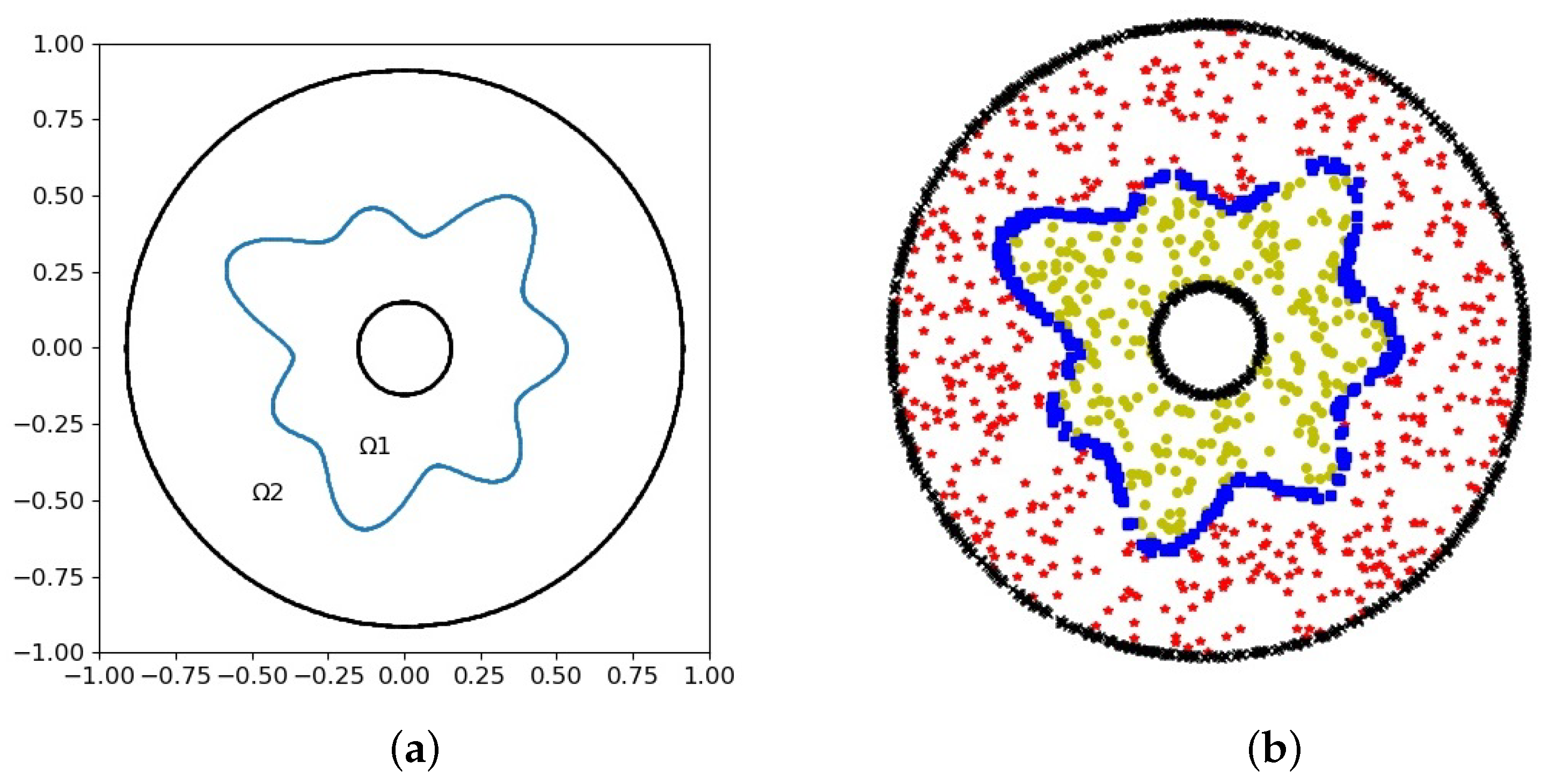
We tested the problems on dual neural networks. Each neural network had 3 layers and each layer had 20 neurons. The geometry of interface $\mathsf{\Gamma }$ and subdomains is illustrated in Figure 8a. The numerical solution was calculated on the uniform sampled points with $N_{r1}=500$, $N_{r2}=300$, $N_{\mathsf{\Gamma }}=300$, and $N_{b1}=200$, $N_{b2}=800$, see Figure 8b. The PINN solution is shown in Figure 9a. The errors between PINN and the exact solutions is shown in Figure 9b. It can be seen that the presented method effectively approximated the solution of the interface problem, and the range of error was from $-2.0\times {10}^{-3}$ to $6.0\times {10}^{-3}$. Figure 10 shows the evolution process of the loss function with adaptive and fixed activation functions for Sub-Net1 and Sub-Net2, respectively.

Table 5. Comparison of errors by adaptive and fixed activation function strategies with different numbers of training points for Example 3.

Activation Function	${\mathit{N}}_{\mathit{\partial }{\mathbf{\Omega }}_1}$/${\mathit{N}}_{\mathit{\partial }{\mathbf{\Omega }}_2}$/${\mathit{N}}_{\mathit{r}1}$/${\mathit{N}}_{\mathit{r}2}$/${\mathit{N}}_{\mathbf{\Gamma }}$	${\mathit{e}}_{{\mathbf{\Omega }}_1}$	${\mathit{e}}_{{\mathbf{\Omega }}_2}$	${\mathit{e}}_{\mathbf{\Gamma }}$	${\mathit{e}}_{\mathit{\partial }{\mathbf{\Omega }}_1}$	${\mathit{e}}_{\mathit{\partial }{\mathbf{\Omega }}_2}$
	$200/50/500/300/75$	2.870 × 10${}^{-3}$	3.765 × 10${}^{-4}$	6.621 × 10${}^{-4}$	3.138 × 10${}^{-4}$	7.113 × 10${}^{-4}$
Adaptive	$400/100/500/300/150$	1.897 × 10${}^{-3}$	2.103 × 10${}^{-4}$	7.083 × 10${}^{-4}$	3.203 × 10${}^{-4}$	4.120 × 10${}^{-4}$
	$800/200/500/300/300$	1.475 × 10${}^{-3}$	2.403 × 10${}^{-4}$	2.853 × 10${}^{-4}$	3.608 × 10${}^{-4}$	2.001 × 10${}^{-4}$
	$200/50/500/300/75$	5.894 × 10${}^{-3}$	5.556 × 10${}^{-4}$	6.790 × 10${}^{-4}$	6.185 × 10${}^{-4}$	5.327 × 10${}^{-4}$
Fixed	$400/100/500/300/150$	5.501 × 10${}^{-3}$	4.778 × 10${}^{-4}$	5.025 × 10${}^{-4}$	5.110 × 10${}^{-4}$	6.311 × 10${}^{-4}$
	$800/200/500/300/300$	4.540 × 10${}^{-3}$	3.633 × 10${}^{-4}$	5.515 × 10${}^{-4}$	5.904 × 10${}^{-4}$	5.522 × 10${}^{-4}$

compares the relative $L_2$ errors with a different number of training points under adaptive and fixed activation functions. We can see that the error decreased with increase in the number of training points on the boundary and interface, and the error of the adaptive activation function method was better than that of the fixed activation function. $e_{\partial {\mathsf{\Omega }}_1}$ and $e_{\partial {\mathsf{\Omega }}_2}$ were the loss errors on the internal and the outer boundary, respectively.

Table 6. Comparison of errors in different terms with different numbers of neurons for Example 3.

Number of Neurons	${\mathit{e}}_{{\mathbf{\Omega }}_1}$	${\mathit{e}}_{{\mathbf{\Omega }}_2}$	${\mathit{e}}_{\mathbf{\Gamma }}$	${\mathit{e}}_{\mathit{\partial }{\mathbf{\Omega }}_1}$	${\mathit{e}}_{\mathit{\partial }{\mathbf{\Omega }}_2}$
10	4.754 × 10${}^{-3}$	9.017 × 10${}^{-4}$	1.550 × 10${}^{-3}$	7.443 × 10${}^{-4}$	1.134 × 10${}^{-3}$
20	2.870 × 10${}^{-3}$	3.765 × 10${}^{-4}$	6.621 × 10${}^{-4}$	3.138 × 10${}^{-4}$	7.113 × 10${}^{-4}$
40	2.282 × 10${}^{-3}$	4.866 × 10${}^{-4}$	8.330 × 10${}^{-4}$	2.915 × 10${}^{-4}$	3.276 × 10${}^{-4}$

illustrates the relative $L_2$ errors of the same training points with a different number of neurons. It is shown that the calculation accuracy increased with increase in the number of neurons.

Example 4.

A two-dimensional elliptic problem with irregular interface geometry.

We tested an interface problem with variable coefficients, and the computational domain is shown in Figure 11. The boundary is given in polar coordinates $r=1.5+0.14sin\left(4\theta \right)+0.12cos\left(6\theta \right)+0.09cos\left(5\theta \right)$, where $\theta \in [0,2\pi )$, and the boundary points are obtained as $x_1=rcos\left(\theta \right)$ and $x_2=rsin\left(\theta \right)$. The computational domain is further divided into two highly irregular, non-convex subdomains, where the interface is given by $r=0.6+0.216sin\left(3\theta \right)+0.096cos\left(2\theta \right)+0.24cos\left(5\theta \right)$ and the corresponding interface points are obtained as $x_1=rcos\left(\theta \right)$ and $x_2=rsin\left(\theta \right)$. The coefficient ${\kappa }^{\pm }$ is defined as

$$\kappa (x,y)=\left\{\begin{array}{c}xy,(x,y)\in {\mathsf{\Omega }}^{+},\hfill \\ x^2+y^2,(x,y)\in {\mathsf{\Omega }}^{-}.\hfill \end{array}\right.$$

(12)

The exact solution is

$$u(x,y)=\left\{\begin{array}{c}sin(x+y),(x,y)\in {\mathsf{\Omega }}^{+},\hfill \\ cos(x+y),(x,y)\in {\mathsf{\Omega }}^{-}.\hfill \end{array}\right.$$

(13)

The necessary forcing term f, boundary and interface conditions are divided from the exact solution.

The geometry of interface $\mathsf{\Gamma }$ and subdomains is illustrated in Figure 11a. The numerical solution was calculated on the uniform sampled points with $N_{r1}=500$, $N_{r2}=300$, $N_{\mathsf{\Gamma }}=300$, and $N_{\partial \mathsf{\Omega }}=800$, see Figure 11b. The balance weights in this example were chosen as ${\omega }_1=0.99999$, ${\omega }_2=0.00001$, ${\omega }_3=0.99999$, ${\omega }_4=0.99999$, ${\omega }_5=0$. The PINN solution is shown in Figure 12a. The error between PINN and exact solutions was between $-1.5\times {10}^{-3}$ and $2.5\times {10}^{-3}$, as shown in Figure 12b. Figure 13 shows the evolution process of the loss function with adaptive and fixed activation functions for Sub-Net1 and Sub-Net2, respectively.

Table 7. Comparison of errors by adaptive and fixed activation function strategies with different numbers of training points for Example 4.

Activation Function	${\mathit{N}}_{\mathit{\partial }\mathbf{\Omega }}$/${\mathit{N}}_{\mathit{r}1}$/${\mathit{N}}_{\mathit{r}2}$/${\mathit{N}}_{\mathbf{\Gamma }}$	${\mathit{e}}_{{\mathbf{\Omega }}_1}$	${\mathit{e}}_{{\mathbf{\Omega }}_2}$	${\mathit{e}}_{\mathbf{\Gamma }}$	${\mathit{e}}_{\mathit{\partial }\mathbf{\Omega }}$
	$200/500/300/75$	1.933 × 10${}^{-4}$	5.989 × 10${}^{-4}$	5.774 × 10${}^{-4}$	3.591 × 10${}^{-4}$
Adaptive	$400/500/300/150$	1.733 × 10${}^{-4}$	3.367 × 10${}^{-4}$	8.803 × 10${}^{-4}$	7.697 × 10${}^{-4}$
	$800/500/300/300$	1.443 × 10${}^{-4}$	1.102 × 10${}^{-4}$	7.815 × 10${}^{-4}$	2.587 × 10${}^{-4}$
	$200/500/300/75$	2.866 × 10${}^{-4}$	6.241 × 10${}^{-4}$	7.144 × 10${}^{-4}$	5.460 × 10${}^{-4}$
Fixed	$400/500/300/150$	3.221 × 10${}^{-4}$	6.001 × 10${}^{-4}$	6.456 × 10${}^{-4}$	4.564 × 10${}^{-4}$
	$800/500/300/300$	2.754 × 10${}^{-4}$	7.596 × 10${}^{-4}$	6.843 × 10${}^{-4}$	3.219 × 10${}^{-4}$

compares the relative $L_2$ errors with different numbers of training points under adaptive activation function and fixed activation function. We can see that the error decreased with increase in the number of training points on the boundary and interface, and the error of the adaptive activation function method was better than that of the fixed activation function.

Table 8. Comparison of errors in different terms with different numbers of neurons for Example 4.

Number of Neurons	${\mathit{e}}_{{\mathbf{\Omega }}_1}$	${\mathit{e}}_{{\mathbf{\Omega }}_2}$	${\mathit{e}}_{\mathbf{\Gamma }}$	${\mathit{e}}_{\mathit{\partial }\mathbf{\Omega }}$
10	3.011 × 10${}^{-4}$	7.143 × 10${}^{-4}$	9.133 × 10${}^{-4}$	5.119 × 10${}^{-4}$
20	1.933 × 10${}^{-4}$	5.989 × 10${}^{-4}$	5.774 × 10${}^{-4}$	3.591 × 10${}^{-4}$
40	2.278 × 10${}^{-4}$	1.473 × 10${}^{-4}$	1.284 × 10${}^{-4}$	4.471 × 10${}^{-4}$

illustrates the relative $L_2$ errors of the same training points with a different number of neurons. It is shown that the calculation accuracy decreased with increase in the number of neurons, but the calculation time cost increased accordingly.

Example 5.

Constant gradient jump over a flat interface.

We also tested a more complicated three-dimensional cube interface problem. Along the z- axis, there were two zones that made up the cube. The conductivity values of the bottom and top sections were 1 and 8 W/m·K, respectively, and the material contact was planar. The prescribed temperatures were 5 and 10 °C along the top and bottom surfaces, respectively, while the remaining surfaces were insulated. Figure 14 depicts the problem’s size and boundary conditions.

With the origin of the Cartesian coordinates system located at the lower front corner of the cubic domain, a distributed heat source $f(x,y,z)=5000(z^2-z+1)$ was applied, yielding the following exact temperature field in the domain:

$$u(x,y,z)=\left\{\begin{array}{c}-33750z^4+833.3z^3-2500z^2+70.9z+10,z<0.05,\hfill \\ -4218.7z^4+104.2z^3-312.5z^2+8.86z+7.56,z\ge 0.05.\hfill \end{array}\right.$$

(14)

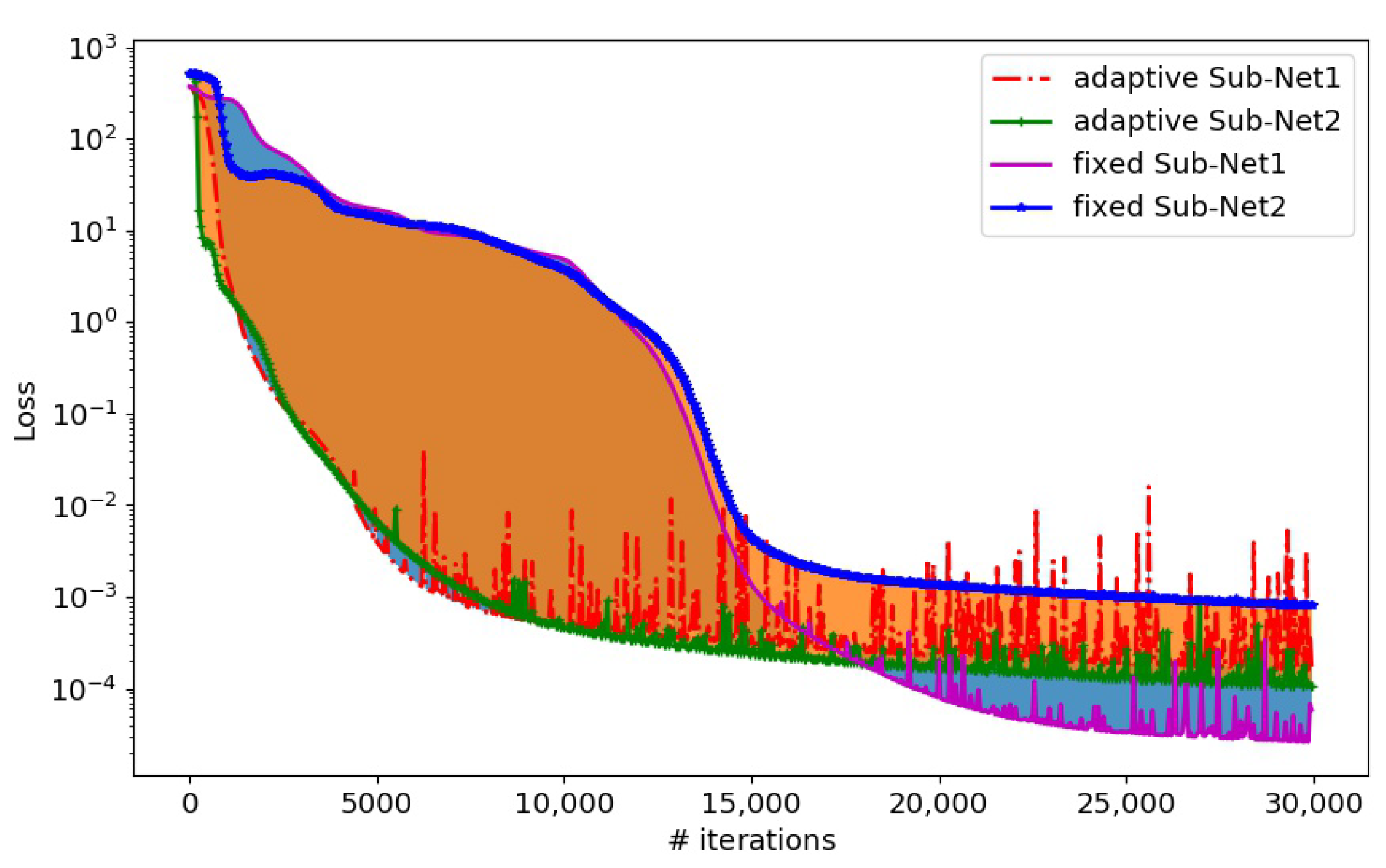
We adopted a dual neural network structure, which included two neural networks. Each network had 3 layers, and each layer had 20 neurons. The numerical solution was calculated on the uniform sampled points with $N_{r1}=2000$, $N_{r2}=2000$, $N_{\mathsf{\Gamma }}=2000$, and $N_{\partial {\mathsf{\Omega }}_1}=3200$, $N_{\partial {\mathsf{\Omega }}_2}=3200$. Figure 15a shows the PINN solution. The balance weights in this problem were chosen as ${\omega }_1=0.00001$, ${\omega }_2=0.99999$, ${\omega }_3=0.99999$, ${\omega }_4=0.99999$, ${\omega }_5=0.99999$. The error between PINN and exact solutions is shown in Figure 15b and the error range was between $-5.0\times {10}^{-3}$ and $1.5\times {10}^{-2}$. This method was shown to accurately approximate the solution of three-dimensional interface problems. Figure 16 shows the evolution process of the loss function with adaptive and fixed activation functions for Sub-Net1 and Sub-Net2, respectively. The effectiveness of the presented algorithm for complex three-dimensional problems on uniform sampling points can be demonstrated by this example.

Table 9. Comparison of errors by adaptive and fixed activation function strategies with different numbers of training points for Example 5.

Activation Function	${\mathit{N}}_{\mathit{\partial }{\mathbf{\Omega }}_1}$/${\mathit{N}}_{\mathit{\partial }{\mathbf{\Omega }}_2}$/${\mathit{N}}_{\mathit{r}1}$/${\mathit{N}}_{\mathit{r}2}$/${\mathit{N}}_{\mathbf{\Gamma }}$	${\mathit{e}}_{{\mathbf{\Omega }}_1}$	${\mathit{e}}_{{\mathbf{\Omega }}_2}$	${\mathit{e}}_{\mathbf{\Gamma }}$	${\mathit{e}}_{\mathit{\partial }{\mathbf{\Omega }}_1}$	${\mathit{e}}_{\mathit{\partial }{\mathbf{\Omega }}_2}$
	$800/800/2000/2000/500$	6.781 × 10${}^{-4}$	1.612 × 10${}^{-3}$	1.711 × 10${}^{-3}$	5.117 × 10${}^{-4}$	9.959 × 10${}^{-4}$
Adaptive	$1600/1600/2000/2000/1000$	5.353 × 10${}^{-4}$	1.144 × 10${}^{-3}$	1.555 × 10${}^{-3}$	4.531 × 10${}^{-4}$	6.983 × 10${}^{-4}$
	$3200/3200/2000/2000/2000$	6.731 × 10${}^{-4}$	1.040 × 10${}^{-3}$	1.415 × 10${}^{-3}$	3.375 × 10${}^{-4}$	7.691 × 10${}^{-4}$
	$800/800/2000/2000/500$	1.457 × 10${}^{-3}$	4.612 × 10${}^{-3}$	4.556 × 10${}^{-3}$	9.456 × 10${}^{-4}$	1.528 × 10${}^{-3}$
Fixed	$1600/1600/2000/2000/1000$	9.458 × 10${}^{-4}$	2.784 × 10${}^{-3}$	3.455 × 10${}^{-3}$	7.781 × 10${}^{-4}$	7.546 × 10${}^{-4}$
	$3200/3200/2000/2000/2000$	8.456 × 10${}^{-4}$	7.458 × 10${}^{-4}$	2.785 × 10${}^{-3}$	3.441 × 10${}^{-4}$	6.745 × 10${}^{-4}$

compares the relative $L_2$ errors with different numbers of training points under the adaptive activation function and the fixed activation function. We can see that the error decreased with increase in the number of training points on the boundary and interface, and the error of the adaptive activation function method was better than that of the fixed activation function.

Table 10. Comparison of errors in different terms with different numbers of neurons for Example 5.

Number of Neurons	${\mathit{e}}_{{\mathbf{\Omega }}_1}$	${\mathit{e}}_{{\mathbf{\Omega }}_2}$	${\mathit{e}}_{\mathbf{\Gamma }}$	${\mathit{e}}_{\mathit{\partial }{\mathbf{\Omega }}_1}$	${\mathit{e}}_{\mathit{\partial }{\mathbf{\Omega }}_2}$
10	1.323 × 10${}^{-3}$	4.117 × 10${}^{-3}$	3.213 × 10${}^{-3}$	9.094 × 10${}^{-4}$	2.362 × 10${}^{-3}$
20	6.781 × 10${}^{-4}$	1.612 × 10${}^{-3}$	1.711 × 10${}^{-3}$	5.117 × 10${}^{-4}$	9.959 × 10${}^{-4}$
40	4.935 × 10${}^{-4}$	8.247 × 10${}^{-4}$	1.203 × 10${}^{-3}$	3.752 × 10${}^{-4}$	4.445 × 10${}^{-4}$

illustrates the relative $L_2$ errors of the same training points with a different number of neurons. It was shown that the calculation accuracy decreased with increase in the number of neurons, but the calculation time cost increased accordingly.

Example 6.

Three-dimensional sphere with a complicated inner region.

Consider a three-dimensional spherical shell with internal and exterior radii of $r_{i}nn=0.151$ and $r_{o}ut=0.911$, respectively, in which there is an immersed-type complex star interface and the interface geometry is given by the level set function shown below.

$$\varphi (x,y,z)=\sqrt{(x^2+y^2+z^2)}-r_0\left(1+{\left(\frac{x^2+y^2}{x^2+y^2+z^2}\right)}^2\sum _{k=1}^3{\beta }_{k}cos\left(n_k(arctan\left(\frac{y}{x}\right)-{\theta }_k)\right)\right),$$

(15)

The exact solution is taken as follows with the same parameters (10) as for the two-dimensional case.

$$u=\left\{\begin{array}{c}\left(16{\left(\frac{y-x}{3}\right)}^5-20{\left(\frac{y-x}{3}\right)}^3+5\left(\frac{y-x}{3}\right)\right)log(x+y+3)cos\left(z\right),(x,y,z)\in {\mathsf{\Omega }}^{+},\hfill \\ sin\left(2x\right)cos\left(2y\right)exp\left(z\right),(x,y,z)\in {\mathsf{\Omega }}^{-}.\hfill \end{array}\right.$$

(16)

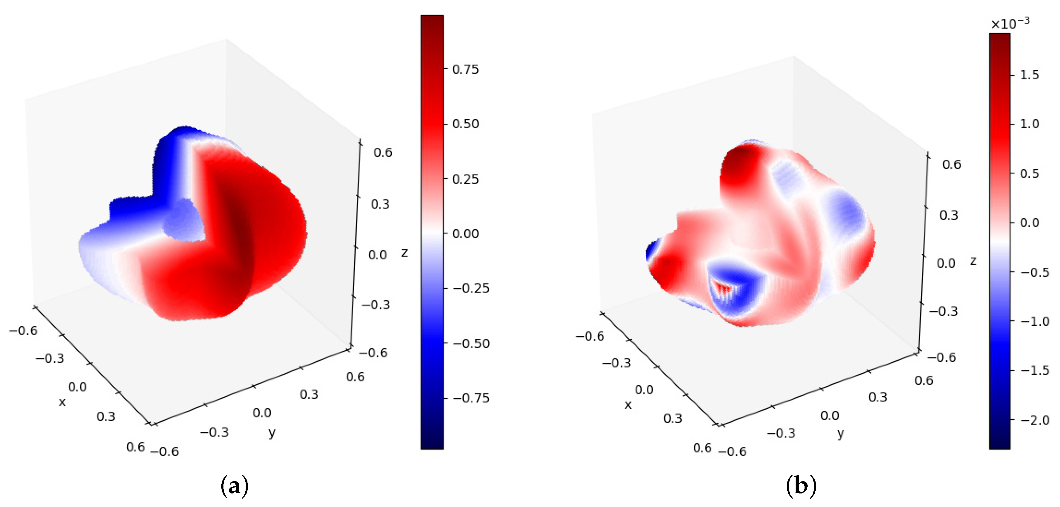
The problem geometry is illustrated in Figure 17.

The numerical solution is calculated on the uniform sampled points with $N_{r1}=500$, $N_{r2}=300$, $N_{\mathsf{\Gamma }}=600$, and $N_{\partial {\mathsf{\Omega }}_1}=400$, $N_{\partial {\mathsf{\Omega }}_2}=400$. The balance weights in the loss function were chosen as ${\omega }_1=0.00001$, ${\omega }_2=0.99999$, ${\omega }_3=0.99999$, ${\omega }_4=0.99999$, ${\omega }_5=0.99999$.

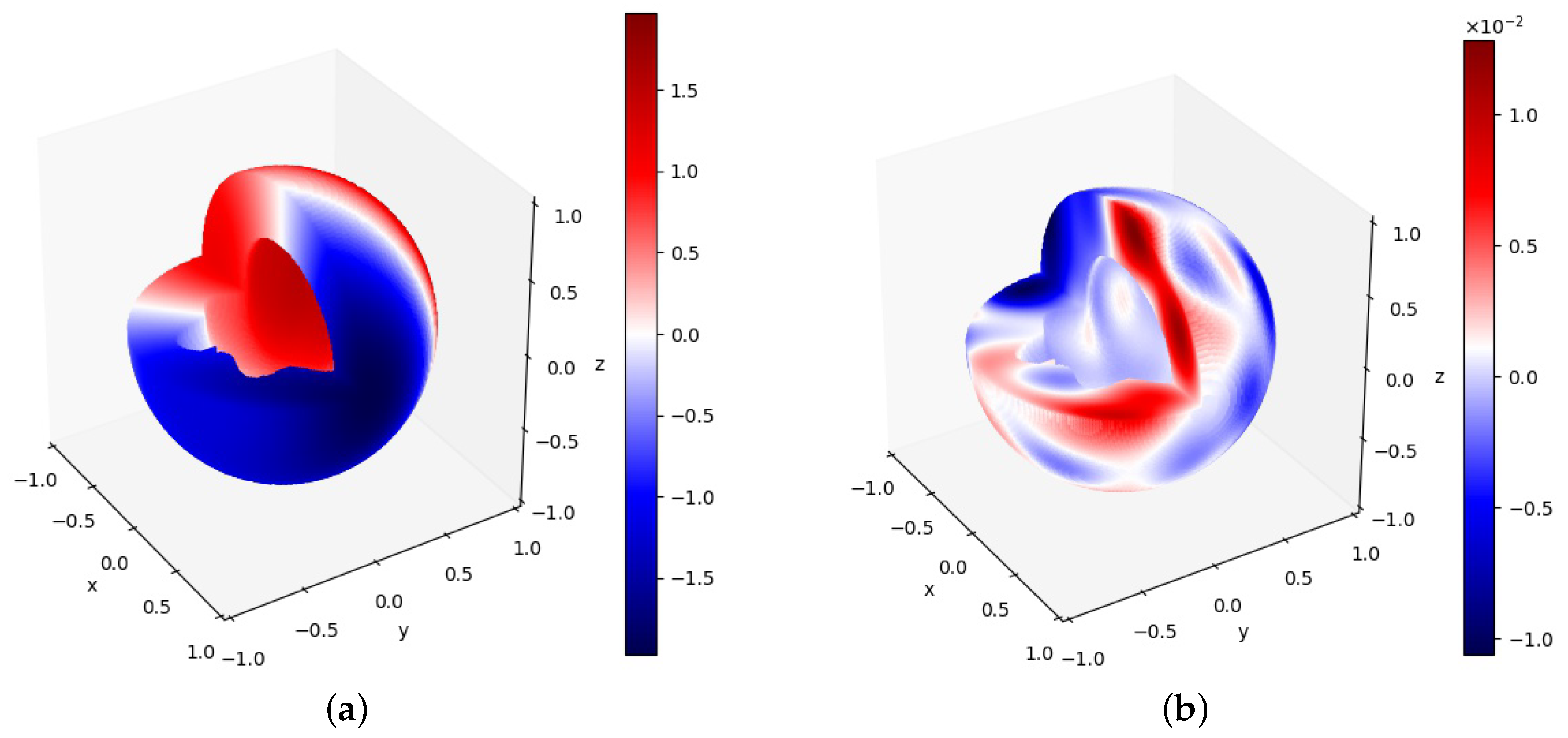
Figure 18a depicts the PINN solution on the domain inside the interface. The error between PINN and the exact solutions in the internal domain is shown in Figure 18b. The relative error range of the internal domain was between $-2.0\times {10}^{-3}$ and $1.5\times {10}^{-3}$. Figure 19a depicted the PINN solution on the domain outside the interface. The error between PINN and the exact solutions in the external domain is shown in Figure 19b. It can be seen that the relative error range of the external domain was between $-1.0\times {10}^{-2}$ and $1.0\times {10}^{-2}$. Figure 20 shows the evolution process of the loss function with adaptive and fixed activation functions for Sub-Net1 and Sub-Net2, respectively.

Table 11. Comparison of errors by adaptive and fixed activation function strategies with different numbers of training points for Example 6.

Activation Function	${\mathit{N}}_{\mathit{\partial }{\mathbf{\Omega }}_1}$/${\mathit{N}}_{\mathit{\partial }{\mathbf{\Omega }}_2}$/${\mathit{N}}_{\mathit{r}1}$/${\mathit{N}}_{\mathit{r}2}$/${\mathit{N}}_{\mathbf{\Gamma }}$	${\mathit{e}}_{{\mathbf{\Omega }}_1}$	${\mathit{e}}_{{\mathbf{\Omega }}_2}$	${\mathit{e}}_{\mathbf{\Gamma }}$	${\mathit{e}}_{\mathit{\partial }{\mathbf{\Omega }}_1}$	${\mathit{e}}_{\mathit{\partial }{\mathbf{\Omega }}_2}$
	$100/100/500/300/150$	4.851 × 10${}^{-3}$	1.075 × 10${}^{-3}$	1.746 × 10${}^{-3}$	7.861 × 10${}^{-3}$	7.923 × 10${}^{-4}$
Adaptive	$200/200/500/300/300$	2.359 × 10${}^{-3}$	6.597 × 10${}^{-4}$	1.036 × 10${}^{-3}$	1.901 × 10${}^{-3}$	4.145 × 10${}^{-4}$
	$400/400/500/300/600$	1.888 × 10${}^{-3}$	5.012 × 10${}^{-4}$	1.167 × 10${}^{-3}$	1.229 × 10${}^{-3}$	3.762 × 10${}^{-4}$
	$100/100/500/300/150$	5.540 × 10${}^{-3}$	2.552 × 10${}^{-3}$	3.290 × 10${}^{-3}$	5.315 × 10${}^{-3}$	2.215 × 10${}^{-3}$
Fixed	$200/200/500/300/300$	4.180 × 10${}^{-3}$	1.576 × 10${}^{-3}$	2.277 × 10${}^{-3}$	3.299 × 10${}^{-3}$	1.561 × 10${}^{-3}$
	$400/400/500/300/600$	2.902 × 10${}^{-3}$	1.337 × 10${}^{-3}$	2.032 × 10${}^{-3}$	1.692 × 10${}^{-3}$	8.895 × 10${}^{-4}$

compares the relative $L_2$ errors with different numbers of training points under the adaptive activation function and the fixed activation function. We can see that the error decreased with increase in the number of training points on the boundary and interface, and the error of the adaptive activation function method was better than that of the fixed activation function.

Table 12. Comparison of errors in different terms with different numbers of neurons for Example 6.

Number of Neurons	${\mathit{e}}_{{\mathbf{\Omega }}_1}$	${\mathit{e}}_{{\mathbf{\Omega }}_2}$	${\mathit{e}}_{\mathbf{\Gamma }}$	${\mathit{e}}_{\mathit{\partial }{\mathbf{\Omega }}_1}$	${\mathit{e}}_{\mathit{\partial }{\mathbf{\Omega }}_2}$
10	5.394 × 10${}^{-3}$	2.087 × 10${}^{-3}$	3.303 × 10${}^{-3}$	7.094 × 10${}^{-3}$	2.062 × 10${}^{-3}$
20	4.851 × 10${}^{-3}$	1.075 × 10${}^{-3}$	1.746 × 10${}^{-3}$	7.861 × 10${}^{-3}$	7.923 × 10${}^{-4}$
40	2.068 × 10${}^{-3}$	1.226 × 10${}^{-3}$	1.637 × 10${}^{-3}$	2.391 × 10${}^{-3}$	6.592 × 10${}^{-4}$

illustrates the relative $L_2$ errors of the same training points with a different number of neurons. It is shown that the calculation accuracy decreased with increase in the number of neurons, but the calculation time cost increased accordingly.

Example 7.

Consider a sphere with an inner doughnut, the level set function of the inner doughnut interface is given as:

$$\varphi (x,y,z)={\left(\sqrt{x^2+y^2}-0.6\right)}^2+z^2-{0.3}^2.$$

(17)

The elliptic coefficients and exact solution are given as prior:

$$\kappa (x,y,z)=\left\{\begin{array}{c}80,(x,y,z)\in {\mathsf{\Omega }}^{+},\hfill \\ 2,(x,y,z)\in {\mathsf{\Omega }}^{-}.\hfill \end{array}\right.$$

(18)

$$u=\left\{\begin{array}{c}xy+x^4+y^4+x{z}^2+cos(2x+y^2+z^3),(x,y,z)\in {\mathsf{\Omega }}^{+},\hfill \\ x^3+x{y}^2+y^3+z^4+sin\left(3(x^2+y^2)\right),(x,y,z)\in {\mathsf{\Omega }}^{-}.\hfill \end{array}\right.$$

(19)

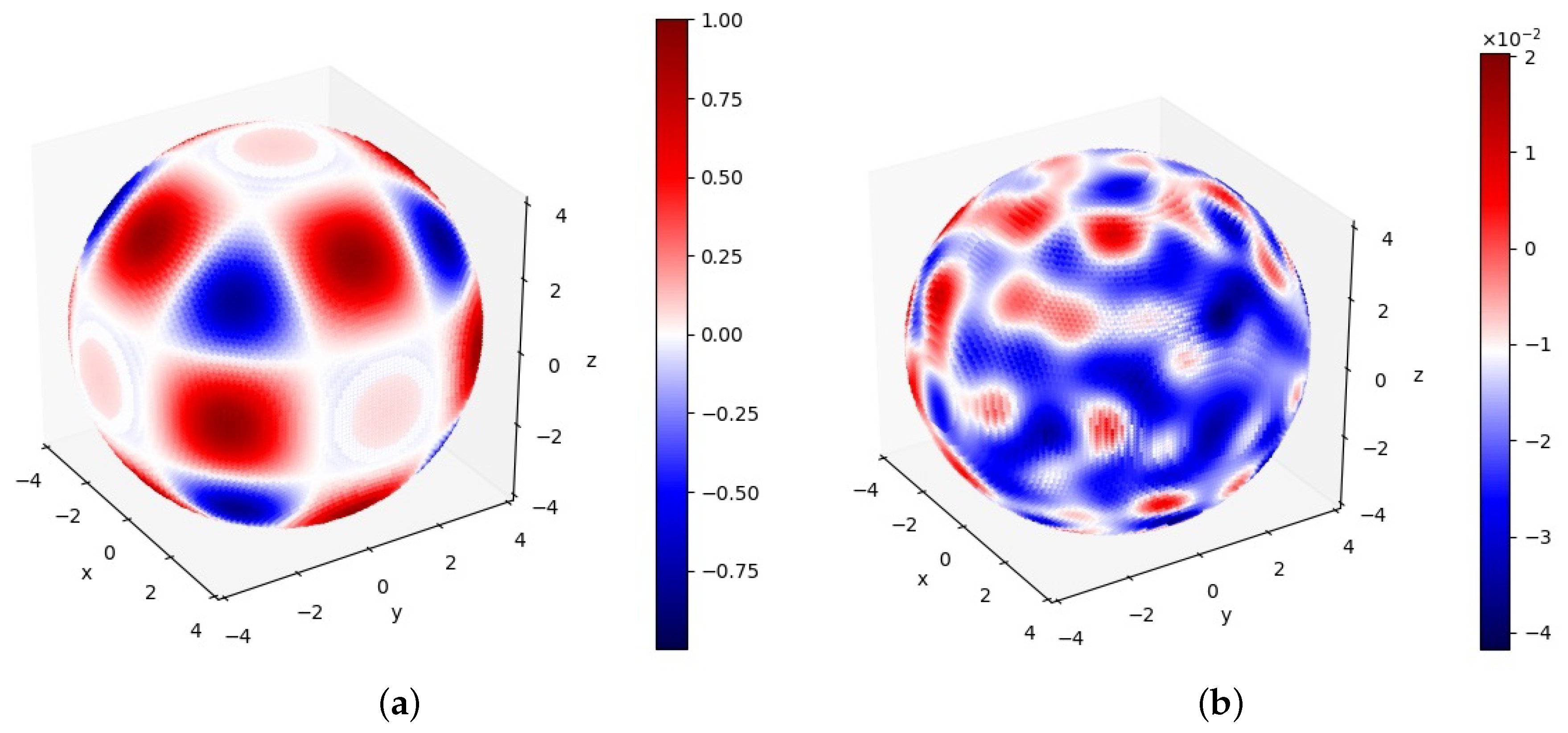
In this problem, a dual neural network structure with two neural networks was adopted. Each network had 4 layers, and each layer had 20 neurons. The numerical solution was calculated on the uniform sampled points with $N_{r1}=2000$, $N_{r2}=300$, $N_{\mathsf{\Gamma }}=300$, and $N_{\partial \mathsf{\Omega }}=2000$. The balance weights were chosen as ${\omega }_1=0.24999$, ${\omega }_2=0.00024$, ${\omega }_3=0.49999$, ${\omega }_4=0.24999$, ${\omega }_5=0$. Figure 21a shows the PINN solution within the interface. The error between PINN and the exact solutions on the internal domain is shown in Figure 21b. It is shown that the relative error range of the internal domain was between $-4\times {10}^{-2}$ and $2\times {10}^{-2}$. Figure 22 plots the PINN solution outside the interface. The errors between PINN and the exact solutions on the external domain is shown in Figure 22b. It can be seen that the relative error range of the external domain was between $-4\times {10}^{-2}$ and $2\times {10}^{-2}$. Figure 23 shows the evolution process of the loss function with adaptive and fixed activation functions for Sub-Net1 and Sub-Net2, respectively.

Table 13. Comparison of errors by adaptive and fixed activation function strategies with different numbers of training points for Example 7.

Activation Functions	${\mathit{N}}_{\mathit{\partial }\mathbf{\Omega }}$/${\mathit{N}}_1$/${\mathit{N}}_2$/${\mathit{N}}_{\mathit{i}}$	${\mathit{e}}_{{\mathbf{\Omega }}_1}$	${\mathit{e}}_{{\mathbf{\Omega }}_2}$	${\mathit{e}}_{\mathbf{\Gamma }}$	${\mathit{e}}_{\mathit{\partial }\mathbf{\Omega }}$
	$500/2000/300/75$	6.022 × 10${}^{-2}$	2.514 × 10${}^{-2}$	3.580 × 10${}^{-2}$	1.011 × 10${}^{-1}$
Adaptive	$1000/2000/300/150$	3.742 × 10${}^{-2}$	1.437 × 10${}^{-2}$	2.165 × 10${}^{-2}$	8.032 × 10${}^{-2}$
	$2000/2000/300/300$	5.330 × 10${}^{-2}$	1.061 × 10${}^{-2}$	1.425 × 10${}^{-2}$	8.363 × 10${}^{-2}$
	$500/2000/300/75$	8.459 × 10${}^{-2}$	6.155 × 10${}^{-2}$	4.486 × 10${}^{-2}$	3.785 × 10${}^{-1}$
Fixed	$1000/2000/300/150$	7.489 × 10${}^{-2}$	4.128 × 10${}^{-2}$	2.445 × 10${}^{-2}$	1.567 × 10${}^{-1}$
	$2000/2000/300/300$	6.446 × 10${}^{-2}$	3.546 × 10${}^{-2}$	3.457 × 10${}^{-2}$	8.458 × 10${}^{-2}$

compares the relative $L_2$ errors with different numbers of training points under the adaptive activation function and the fixed activation function. We can see that the error decreased with increase in the number of training points on the boundary and interface, and the error of the adaptive activation function method was better than that of the fixed activation function.

Table 14. Comparison of errors in different terms with different numbers of neurons for Example 7.

Number of Neurons	${\mathit{e}}_{{\mathbf{\Omega }}_1}$	${\mathit{e}}_{{\mathbf{\Omega }}_2}$	${\mathit{e}}_{\mathbf{\Gamma }}$	${\mathit{e}}_{\mathit{\partial }\mathbf{\Omega }}$
10	6.125 × 10${}^{-2}$	3.221 × 10${}^{-2}$	4.208 × 10${}^{-2}$	9.971 × 10${}^{-2}$
20	5.330 × 10${}^{-2}$	1.061 × 10${}^{-2}$	1.425 × 10${}^{-2}$	8.363 × 10${}^{-2}$
40	2.175 × 10${}^{-2}$	7.691 × 10${}^{-3}$	1.228 × 10${}^{-2}$	2.674 × 10${}^{-2}$

illustrates the relative $L_2$ errors of the same training points with a different number of neurons. It is shown that the calculation accuracy decreased with increase in the number of neurons, while the calculation time cost increased accordingly.

6. Conclusions

A soft constraint physics-informed neural network is proposed to solve nonhomogeneous elliptic interface problems. Due to the complexity of geometry, the solution may change dramatically across the interface. Traditional numerical methods for solving these problems are challenging. As the interface divides the computational domain into two disjoint parts, a dual neural network structure with two separate neural networks in two disjoint subdomains is employed. The two neural networks are joined by jumping conditions on the interface, which are necessary to capture the solution singularity on the interface. The PDEs, boundary conditions and jump condition on the interface are then formulated into the loss function by PINN, and the terms in the loss function balanced by penalty weights. An adaptive activation function method is used to increase the computing efficiency in more difficult situations. This method may be optimized by dynamically changing the topology of the loss function used in the optimization process to attain the optimal network performance. Numerical experiments for 2D and 3D situations demonstrated that the proposed method can solve interface problems with flexibility, effectiveness, and enough accuracy.

References

1. Oevermann, M.; Scharfenberg, C.; Klein, R. A sharp interface finite volume method for elliptic equations on Cartesian grids. J. Comput. Phys. 2009, 228, 5184–5206. [Google Scholar] [CrossRef] [Green Version]
2. Preskill, B.; Sethian, J.A. Jump splicing schemes for elliptic interface problems and the incompressible Navier-Stokes equations. arXiv 2016, arXiv:1612.09342. [Google Scholar]
3. Guyomarc’h, G.; Lee, C.O.; Jeon, K. A discontinuous Galerkin method for elliptic interface problems with application to electroporation. Commun. Numer. Methods Eng. 2009, 25, 991–1008. [Google Scholar] [CrossRef]
4. López-Ruiz, G.; Bravo-Castillero, J.; Brenner, R.; Cruz, M.E.; Guinovart-Díaz, R.; Pérez-Fernández, L.D.; Rodríguez-Ramos, R. Variational bounds in composites with nonuniform interfacial thermal resistance. Appl. Math. Model. 2015, 39, 7266–7276. [Google Scholar] [CrossRef]
5. Rocha, R.P.A.; Cruz, M.E. Computation of the effective conductivity of unidirectional fibrous composites with an interfacial thermal resistance. Numer. Heat Transf. Part A Appl. 2001, 39, 179–203. [Google Scholar] [CrossRef]
6. Costa, R.; Nobrega, J.M.; Clain, S.; Machado, G.J. Very high-order accurate polygonal mesh finite volume scheme for conjugate heat transfer problems with curved interfaces and imperfect contacts. Comput. Methods Appl. Mech. Eng. 2019, 357, 112560. [Google Scholar] [CrossRef]
7. Meften, G.A.; Ali, A.H. Continuous dependence for double diffusive convection in a Brinkman model with variable viscosity. Acta Univ. Sapientiae Math. 2022, 14, 125–146. [Google Scholar] [CrossRef]
8. Meften, G.A.; Ali, A.H.; Yaseen, M.T. Continuous dependence for thermal convection in a Forchheimer-Brinkman model with variable viscosity. AIP Conf. Proc. 2023, 2457, 020005. [Google Scholar]
9. Huang, P.; Wu, H.; Xiao, Y. An unfitted interface penalty finite element method for elliptic interface problems. Comput. Methods Appl. Mech. Eng. 2017, 323, 439–460. [Google Scholar] [CrossRef]
10. Barrett, J.; Elliott, C. Fitted and unfitted finite element methods for elliptic equations with smooth interfaces. IMA J. Numer. Anal. 1987, 7, 283–300. [Google Scholar] [CrossRef]
11. Guo, H.; Yang, X. Gradient recovery for elliptic interface problem: I. body-fitted mesh. arXiv 2016, arXiv:1607.05898. [Google Scholar] [CrossRef]
12. Li, J.; Wohlmuth, J.M.J.B.; Zou, J. Optimal a priori estimates for higher order finite elements for elliptic interface problems. Appl. Numer. Math. 2010, 60, 19–37. [Google Scholar] [CrossRef]
13. Zheng, X.; Lowengrub, J. An interface-fitted adaptive mesh method for elliptic problems and its application in free interface problems with surface tension. Adv. Comput. Math. 2016, 42, 1225–1257. [Google Scholar] [CrossRef]
14. Cao, F.; Sheng, Z.; Yuan, G. Monotone finite volume schemes for diffusion equation with imperfect interface on distorted meshes. J. Sci. Comput. 2018, 76, 1055–1077. [Google Scholar] [CrossRef]
15. Peskin, C. Numerical analysis of blood flow in the heart. J. Comput. Phys. 1977, 25, 220–252. [Google Scholar] [CrossRef]
16. Li, Z.; Ito, K. The Immersed Interface Method: Numerical Solutions of PDEs Involving Interfaces and Irregular Domains; Society for Industrial and Applied Mathematics: Philadelphia, PA, USA, 2006. [Google Scholar]
17. Ji, H.; Zhang, Q.; Wang, Q.; Xie, Y. A partially penalised immersed finite element method for elliptic interface problems with non-homogeneous jump conditions. East Asia J. Appl. Math. 2018, 8, 1–23. [Google Scholar] [CrossRef] [Green Version]
18. Wu, H.; Xiao, Y. An unfitted hp-interface penalty finite element method for elliptic interface problems. J. Comput. Math. 2019, 37, 316. [Google Scholar]
19. Guo, R.; Lin, T. A higher degree immersed finite element method based on a Cauchy extension for elliptic interface problems. SIAM J. Numer. Anal. 2019, 57, 1545–1573. [Google Scholar] [CrossRef]
20. Wang, Q.; Zhang, Z.; Wang, L. New immersed finite volume element method for elliptic interface problems with non-homogeneous jump conditions. J. Comput. Phys. 2020, 427, 110075. [Google Scholar] [CrossRef]
21. Weinan, E.; Yu, B. The Deep Ritz Method: A Deep Learning-Based Numerical Algorithm for Solving Variational Problems. Commun. Math. Stat. 2017, 6, 1–12. [Google Scholar]
22. Sirignano, J.A.; Konstantinos, S. DGM: A deep learning algorithm for solving partial differential equations. J. Comput. Phys. 2018, 375, 1339–1364. [Google Scholar] [CrossRef] [Green Version]
23. Raissi, M.; Perdikaris, P.; Karniadakis, G.E. Physics-informed neural network: A deep learning framework for solving forward and inverse problems involving nonlinear partial differential equations. J. Comput. Phys. 2019, 378, 686–707. [Google Scholar] [CrossRef]
24. Lu, L.; Meng, X.; Mao, Z.; Karniadakis, G.E. DeepXDE: A deep learning library for solving differential equations. SIAM Rev. 2021, 63, 208–228. [Google Scholar] [CrossRef]
25. Pang, G.; Lu, L.; Karniadakis, G.E. fPINNs: Fractional physics-informed neural networks. SIAM J. Sci. Comput. 2019, 41, A2603–A2626. [Google Scholar] [CrossRef] [Green Version]
26. Zhang, D.; Lu, L.; Guo, L.; Karniadakis, G.E. Quantifying total uncertainty in physics-informed neural networks for solving forward and inverse stochastic problems. J. Comput. Phys. 2019, 397, 108850. [Google Scholar] [CrossRef] [Green Version]
27. Zhang, D.; Guo, L.; Karniadakis, G.E. Learning in modal space: Solving time-dependent stochastic PDEs using physics-informed neural networks. SIAM J. Sci. Comput. 2020, 42, A639–A665. [Google Scholar] [CrossRef]
28. Chen, Y.; Lu, L.; Karniadakis, G.E.; Negro, L.D. Physics-informed neural networks for inverse problems in nano-optics and metamaterials. Opt. Express 2020, 28, 11618–11633. [Google Scholar] [CrossRef] [Green Version]
29. Lu, L.; Pestourie, R.; Yao, W.; Wang, Z.; Verdugo, F.; Johnson, S.G. Physics-informed neural networks with hard constraints for inverse design. arXiv 2021, arXiv:2102.04626. [Google Scholar] [CrossRef]
30. Raissi, M.; Yazdani, A.; Karniadakis, G.E. Hidden fluid mechanics: Learning velocity and pressure fields from flow visualizations. Science 2020, 367, 1026–1030. [Google Scholar] [CrossRef]
31. Yazdani, A.; Lu, L.; Raissi, M.; Karniadakis, G.E. Systems biology informed deep learning for inferring parameters and hidden dynamics. PLoS Comput. Biol. 2020, 16, e1007575. [Google Scholar] [CrossRef]
32. Jagtap, A.D.; Karniadakis, G.E. Extended physics-informed neural networks (xpinns): A generalized space-time domain decomposition based deep learning framework for nonlinear partial differential equations. Commun. Comput. Phys. 2020, 28, 2002–2041. [Google Scholar]
33. Jagtap, A.D.; Kharazmi, E.; Karniadakis, G.E. Conservative physics-informed neural networks on discrete domains for conservation laws: Applications to forward and inverse problems. Comput. Methods Appl. Mech. Eng. 2020, 365, 113028. [Google Scholar] [CrossRef]
34. Li, W.; Xiang, X.; Xu, Y. Deep domain decomposition method: Elliptic problems. PMLR 2020, 107, 269–286. [Google Scholar]
35. Wang, Z.J.; Zhang, Z.W. A mesh-free method for interface problems using the deep learning approach. J. Comput. Phys. 2020, 400, 108963. [Google Scholar] [CrossRef]
36. Hu, W.F.; Lin, T.S.; Lai, M.C. A discontinuity capturing shallow neural network for elliptic interface problems. arXiv 2021, arXiv:2106.05587. [Google Scholar] [CrossRef]
37. He, C.Y.; Hu, X.Z.; Mu, L. A mesh-free method using piecewise deep neural network for elliptic interface problems. J. Comput. Appl. Math. 2022, 412, 114358. [Google Scholar] [CrossRef]
38. Wu, S.D.; Zhu, A.Q.; Tang, Y.F.; Lu, B.Z. On convergence of neural network methods for solving elliptic interface problems. arXiv 2022, arXiv:2203.03407v2. [Google Scholar]
39. Jagtap, A.D.; Kawaguchi, K.; Karniadakis, G.E. Locally adaptive activation functions with slope recovery term for deep and physics-informed neural networks. Proc. R. Soc. A 2020, 476, 20200334. [Google Scholar] [CrossRef]
40. Jagtap, A.D.; Kawaguchi, K.; Karniadakis, G.E. Adaptive activation functions accelerate convergence in deep and physics-informed neural networks. J. Comput. Phys. 2020, 404, 109136. [Google Scholar] [CrossRef] [Green Version]
41. Wang, S.F.; Yu, X.L.; Perdikaris, P. When and why PINNs fail to train: A neural tangent kernel perspective. J. Comput. Phys. 2022, 449, 110768. [Google Scholar] [CrossRef]
42. McClenny, L.D.; Braga-Neto, U.M. Self-Adaptive Physics-Informed Neural Networks using a Soft Attention Mechanism. arXiv 2022, arXiv:2009.04544. [Google Scholar]
43. van der Meer, R.; Oosterlee, C.W.; Borovykh, A. Optimally weighted loss functions for solving PDEs with Neural Networks. J. Comput. Appl. Math. 2022, 405, 113887. [Google Scholar] [CrossRef]
Figure 1. Schematic duel PINNs for interface problems. Two independent neural networks are constructed to approximate solutions to two subdomains, respectively.
Mathematics 11 01843 g001
Figure 2. (a) Computational domain and interface geometry and (b) training points.
Mathematics 11 01843 g002
Figure 3. (a) The PINN solution and (b) the error between PINN and exact solutions for Example 1.
Mathematics 11 01843 g003
Figure 4. The evolution of loss error for Example 1.
Mathematics 11 01843 g004
Figure 5. (a) Domain and interface geometry and (b) training points.
Mathematics 11 01843 g005
Figure 6. (a) The PINN solution and (b) the error between PINN and the exact solution for Example 2.
Mathematics 11 01843 g006
Figure 7. The evolution of average loss error for Example 2.
Mathematics 11 01843 g007
Figure 8. (a) Problem geometry and (b) training points.
Mathematics 11 01843 g008
Figure 9. (a) The PINN solution and (b) the error between PINN and exact solutions for Exampe 3.
Mathematics 11 01843 g009
Figure 10. The evolution plot of loss L 2 error for Example 3.
Mathematics 11 01843 g010
Figure 11. (a) Computational domain and interface shape and (b) training points.
Mathematics 11 01843 g011
Figure 12. (a) The PINN solution and (b) the error between PINN and the exact solution for Example 4.
Mathematics 11 01843 g012
Figure 13. The plot of L s average error loss for Example 4.
Mathematics 11 01843 g013
Figure 14. Physical model and interface geometry.
Mathematics 11 01843 g014
Figure 15. (a) The PINN solution and (b) the error between PINN and exact solution for Example 5.
Mathematics 11 01843 g015
Figure 16. The plot of L s average error loss for Example 5.
Mathematics 11 01843 g016
Figure 17. Computational geometry and interface.
Mathematics 11 01843 g017
Figure 18. (a) The PINN solution and (b) the error between PINN and the exact solution for internal domain.
Mathematics 11 01843 g018
Figure 19. (a) The PINN solution and (b) the error between PINN and exact solution for external domain.
Mathematics 11 01843 g019
Figure 20. The evolution of L s average error loss for Example 6.
Mathematics 11 01843 g020
Figure 21. (a) The PINN solution and (b) the error between PINN and the exact solution on external area.
Mathematics 11 01843 g021
Figure 22. (a) The PINN solution and (b) the error between PINN and the exact solution on internal domain.
Mathematics 11 01843 g022
Figure 23. The plot of L s average error loss for Example 7.
Mathematics 11 01843 g023