The Dynamical Behavior of a Three-Dimensional System of Exponential Difference Equations

Abstract

The boundedness nature and persistence, global and local behavior, and rate of convergence of positive solutions of a second-order system of exponential difference equations, is investigated in this work. Where the parameters $A,B,C,\alpha ,\beta ,\gamma ,\delta ,\eta$, and $\xi$are constants that are positive, and the initials $U_{-1},U_0,V_{-1},V_0,W_{-1}$, and $W_0$ are non-negative real numbers. Some examples are provided to support our theoretical results.

1. Introduction

1.1. Motivation and Literature Review

Differential equations have discrete analogs in difference equations. On their own, linear and nonlinear difference equations, their stability analysis, and local and global behaviors are fascinating (See [1,2,3,4,5,6,7] and references therein). Exponential difference equations first appeared in population dynamics. Though their analysis is difficult, it is also incredibly interesting.

Biologists feel that understanding population dynamics requires a thorough understanding of equilibrium points and their stability. Furthermore, difference equations have several applications in finance, biology, physics, and social sciences. The dynamics of discrete dynamical systems in the exponential form are rich. Population models can be discussed using such systems. Discrete dynamical systems outperform related systems in differential equations, due to their superior computing ability. Difference equations are larger, opposed to looking at the behavior of population models, in the event of non-overlapping generations [8,9]. Difference equations are mathematical equations that describe the relationship between a sequence of values. They are important in many fields, including economics, physics, engineering, and computer science. Here are some of the key reasons why difference equations are important:

Modeling dynamic systems [10]: Difference equations are often used to model dynamic systems, such as population growth, stock prices, or the spread of infectious diseases. By describing the relationship between the values of a sequence over time, these equations help researchers to understand how these systems behave.

Numerical Analysis [11]: Difference equations are also useful in numerical analysis, which involves using numerical methods to approximate solutions to mathematical problems. In particular, difference equations can be used to approximate the solutions to differential equations, which are more difficult to solve analytically.

Control Theory [12]: Difference equations are used extensively in control theory, which involves designing systems that can respond to changes in their environment or inputs. By describing the relationship between the current state of a system and its previous states, difference equations help engineers to design feedback systems that can adjust their behavior to achieve desired outcomes.

Computer Science [13,14]: Difference equations are used in computer science to model algorithms and data structures. For example, the recurrence relation for the Fibonacci sequence, is a difference equation that describes how to compute the nth number in the sequence, using the values of the previous two numbers.

Overall, difference equations are an important tool for modeling and analyzing dynamic systems, approximating solutions to mathematical problems, designing feedback systems, and modeling algorithms and data structures in computer science.

Analyzing the dynamics of solutions to systems of difference equations, and discussing the local and global asymptotic stability of their equilibriums, is interesting [10,12,13,15,16,17,18]. The authors in [19], obtained the behavior of solutions to the difference equation:

$$U_{m+1}=a{U}_m+b{U}_{m-1}{e}^{-U_m},m=0,1,\dots$$

where the initials $U_{-1}$ and $U_0$ are positive numbers, and the constants a and b are positive. This equation can be called a biological model. Furthermore, the authors investigated equivalent conclusions for the system of difference equations in [20]:

$$U_{m+1}=a{V}_m+b{U}_{m-1}{e}^{-V_m},V_{m+1}=c{U}_m+d{V}_{m-1}{e}^{-U_m}$$

where the initials $U_{-1},U_0,V_{-1},V_0$ are positive numbers and the constants $a,b,c,d$ are positive.

The authors found conclusions for the behavior of positive solutions for the following system in [21]

$$U_{m+1}=a{U}_m+b{V}_{m-1}{e}^{-U_m},V_{m+1}=c{V}_m+d{U}_{m-1}{e}^{-V_m}$$

where $a,b,c,d$ are positive constants and the: initials $U_{-1},U_0,V_{-1},V_0$ are also positive numbers.

In [1], the authors studied

$$U_{m+1}=a+b{U}_{m-1}{e}^{-U_m}$$

where b and a are positive constants and the initials $U_{-1}$ and $U_o$ are positive numbers.

In [2], the authors investigated the behavior of

$$\begin{array}{c}\hfill U_{m+1}=a+b{U}_{m-1}{e}^{-V_m}\\ \hfill V_{m+1}=c+d{V}_{m-1}{e}^{-U_m}\end{array}$$

In [22], the authors looked into the behavior of

$$\begin{array}{c}\hfill U_{m+1}=a+b{U}_{m-1}+c{U}_{m-1}{e}^{-V_m},\\ \hfill V_{m+1}=\alpha +\beta V_{m-1}+\gamma V_{m-1}{e}^{-U_m}.\end{array}$$

where $a,b,c,\alpha ,\beta ,\gamma$are positive constants, and the initials $U_{-1},$$U_o,$$V_{-1},$$V_o$ are positive real values.

Motivated by the above papers, we will extend the difference equation in [1], the system in [2], and the system in [22], to the following system:

$$U_{m+1}=A+B{U}_{m-1}+C{U}_{m-1}{e}^{-V_m}$$

$$V_{m+1}=\alpha +\beta V_{m-1}+\gamma V_{m-1}{e}^{-W_m}$$

$$W_{m+1}=\delta +\eta W_{m-1}+\xi W_{m-1}{e}^{-U_m}$$

(1)

where $\alpha ,\beta ,\gamma ,\delta ,\eta ,\xi ,A,B,C$ are positive constants, and the initials $U_{-1},U_0,V_{-1},V_0,$$W_{-1},W_0$ are positive real values.

The aim of this work is to look at the persistence, boundedness, and asymptotic behavior of the system’s positive solutions $\left(1\right)$.

It is clear that in the specific instances when $B=\beta =\eta =0$, $\left(1\right)$ becomes the system in [2]. Thus, we obtain the difference equation in [1] when $U_m=V_m=W_m,A=\alpha =\delta ,B=\beta =\eta =0,C=\gamma =\xi$. The following works discuss differences and systems of difference equations in exponential form: [1,2,19,20,21,22,23,24,25]. Furthermore, because difference equations have several applications in applied sciences, many papers and books on the theory of difference equations may be found, e.g., see [8,26,27] and references therein.

1.2. Structure of the Paper

The structure of this paper will be as follows: In Section 2, we study the asymptotic solution of system (1), by investigating its boundedness and persistence. In Theorem 2, we establish an invariant set of intervals of system $\left(1\right)$. Theorems 3 and 4 deal with the local stability of the system and prove that every solution converges to its equilibrium point. Theorem 5 deals with the global stability of the system. In Section 3, we present some interesting numerical examples, that show the behavior of the solution of system $\left(1\right)$.

2. Main Results

Asymptotic Behavior of Solutions of System $\left(1\right)$

First, the persistence and boundedness of the solutions must be established; in the first theorem, we will compare the persistence and boundedness of positive solutions of $\left(1\right)$, with solutions of a solvable system of difference equations. Our approach is based on Theorem 2 from [28]. See [2,8,27] for related and comparable results.

Theorem 1. 

Consider system $\left(1\right)$ such that:

$$e^{-\delta }\gamma +\beta <1,e^{-\alpha }C+B<1,\xi e^{-A}+\eta <1.$$

(2)

Then, every positive solution of $\left(1\right)$ is bounded and persists.

Proof. 

Let $(U_m,V_m,W_m)$ be any arbitrary solution of $\left(1\right)$. We may deduce as a result of $\left(1\right)$

$$U_m\ge A,V_m\ge \alpha ,W_m\ge \delta ,m=1,2,\dots$$

(3)

In addition, it follows from $\left(1\right)$ and $\left(3\right)$ that,

$$U_{m+1}\le A+B{U}_{m-1}+C{U}_{m-1}{e}^{-\alpha },V_{m+1}\le \alpha +\beta V_{m-1}+\gamma V_{m-1}{e}^{-\delta },$$

$$W_{m+1}\le \delta +\eta W_{m-1}+\xi W_{m-1}{e}^{-A},m=0,1,2,\dots$$

(4)

The non-homogeneous difference equations will be considered next

$$u_{m+1}=A+B{u}_{m-1}+C{u}_{m-1}{e}^{-\alpha },v_{m+1}=\alpha +\beta v_{m-1}+\gamma V_{m-1}{e}^{{-}_{\delta }},$$

$$w_{m+1}=\delta +\eta w_{m-1}+\xi w_{m-1}{e}^{-A},m=0,1,2,\dots$$

(5)

Therefore, a solution $(u_m,v_m,w_m)$ of $\left(5\right)$ is provided by

$$u_m=r_1{(e^{-\alpha }C+B)}^{m/2}+r_2{(-1)}^m{(e^{-\alpha }C+B)}^{m/2}+\frac{A}{1-e^{-\alpha }C-B}$$

$$v_m=s_1{(e^{-\delta }\gamma +\beta )}^{m/2}+s_2{(-1)}^m{(\beta +\gamma e^{-\delta })}^{m/2}+\frac{\alpha }{1-e^{-\delta }\gamma -\beta }$$

$$w_m=t_1{(\xi e^{-A}+\eta )}^{m/2}+t_2{(-1)}^m{(\xi e^{-A}+\eta )}^{m/2}+\frac{\delta }{-\eta +1-\xi e^{-\alpha }},m=1,2,\dots$$

(6)

where $r_1,r_2,s_1,s_2,t_1,t_2$depend on the initial values $v_0,u_0,v_{-1},w_{-1},w_0,u_{-1}.$ Thus, $u_m,v_m$and $w_m$ are bounded sequences. Now, we consider $(u_m,v_m,w_m)$ of $\left(5\right)$, such that

$$u_{-1}=U_{-1},u_0=U_0,v_{-1}=V_{-1},v_0=V_0,w_{-1}=W_{-1},w_0=W_0$$

(7)

Thus, from $\left(4\right)$ and $\left(7\right)$, we get

$$U_m\le u_m,V_m\le v_m,W_m\le w_m,m=1,2,\dots$$

(8)

Therefore, $U_m,V_m$, and $W_m$ are bounded sequences. Hence, from $\left(3\right)$, the proof of this theorem is now complete. □

Theorem 2. 

Consider system $\left(1\right)$ with relations $\left(2\right)$ satisfied. Then, the following statements are true: $\left(i\right)$ The set

$$\left[A,\frac{A}{1-e^{-\alpha }C-B}\right]\times \left[\alpha ,\frac{\alpha }{1-e^{-\delta }\gamma -\beta }\right]\times \left[\delta ,\frac{\delta }{-\eta +1-\xi e^{-A}}\right]$$

is an invariant set of $\left(1\right).$

$\left(ii\right)$ Let ϵ be a positive number, and $(U_m,V_m,W_m)$ be a solution of $\left(1\right).$

Consider

$$I_1=\left[A,\frac{A+ϵ}{1-e^{-\alpha }C-B}\right],I_2=\left[\alpha ,\frac{\alpha +ϵ}{-\beta +1-\gamma e^{-\delta }}\right],I_3=\left[\delta ,\frac{\delta +ϵ}{-\eta +1-\xi e^{-A}}\right].$$

(9)

Then, there exists $m_0$, provided that ∀ $m\ge m_0$

$$U_m\in I_1,V_m\in I_2,W_m\in I_3.$$

(10)

Proof. 

(i) Let $(U_m,V_m,W_m)$ be a solution of $\left(1\right)$ with $U_{-1},U_0,V_{-1},V_0,W_{-1},W_0$, such that

$$U_{-1},U_0\in \left[A,\frac{A}{1-e^{-\alpha }C-B}\right],V_{-1},V_0\in \left[\alpha ,\frac{\alpha }{-\beta +1-\gamma e^{-\delta }}\right],W_{-1},W_0\in \left[\delta ,\frac{\delta }{-\eta +1-\xi e^{-A}}\right]$$

(11)

Then, from $\left(1\right)$ and $\left(11\right)$ we have:

$$\begin{array}{c}\hfill A\le U_1=A+B{U}_{-1}+C{U}_{-1}{e}^{-V_0}\le A\left[1+\frac{1}{1-e^{-\alpha }C-B}(e^{-\alpha }C+B)\right]=\frac{A}{1-e^{-\alpha }C-B},\\ \hfill \alpha \le V_1=\alpha +\beta V_{-1}+\gamma V_{-1}{e}^{-W_0}\le \alpha \left[1+\frac{1}{1-e^{-\delta }\gamma -\beta }(e^{-\delta }\gamma +\beta )\right]=\frac{\alpha }{1-e^{-\delta }\gamma -\beta },\\ \hfill \delta \le W_1=\delta +\eta W_{-1}+\xi W_{-1}{e}^{-U_0}\le \delta \left[1+\frac{1}{-\eta +1-\xi e^{-A}}(\xi e^{-A}+\eta )\right]=\frac{\delta }{-\eta +1-\xi e^{-A}}.\end{array}$$

Then,

$$\begin{array}{c}\hfill A\le U_m\le \frac{A}{1-e^{-\alpha }C-B},\\ \hfill \alpha \le V_m\le \frac{\alpha }{1-e^{-\delta }\gamma -\beta },\\ \hfill \delta \le W_m\le \frac{\delta }{-\eta +1-\xi e^{-A}},m=1,2,3,\dots \end{array}$$

$\left(ii\right)$ Let $(U_m,V_m,W_m)$ be a solution of $\left(1\right).$ Therefore, from Theorem 1 we get,

$$0<l_1=\underset{m\to \infty }{Lim}inf{U}_m,0<l_2=\underset{m\to \infty }{Lim}inf{V}_m,0<l_3=\underset{m\to \infty }{Lim}inf{W}_m,$$

$$0<L_1=\underset{m\to \infty }{Lim}sup{U}_m<\infty ,0<L_2=\underset{m\to \infty }{Lim}sup{V}_m<\infty ,0<L_3=\underset{m\to \infty }{Lim}sup{W}_m<\infty .$$

(12)

We get,

$$L_1\le A+B{L}_1+C{L}_1{e}^{-l_2},L_2\le \alpha +\beta L_2+\gamma L_2{e}^{-l_3},L_3\le \delta +\eta L_3+\xi L_3{e}^{-l_1}$$

$$\begin{array}{ccc}\hfill l_1& \ge & A+B{l}_1+C{l}_1{e}^{-L_2},l_2\ge \alpha +\beta l_2+\gamma l_2{e}^{-L_3},l_3\ge \delta +\eta l_3+\xi l_3{e}^{-L_1}\hfill \end{array}$$

which imply that

$$A\le L_1\le \frac{A}{1-e^{-\alpha }C-B},\alpha \le L_2\le \frac{\alpha }{1-e^{-\delta }\gamma -\beta },\delta \le L_3\le \frac{\delta }{-\eta +1-\xi e^{-A}}$$

(13)

Thus, from $\left(1\right)$, there exists $m_0$ such that $\left(10\right)$ holds true. This completes the proof of the theorem. □

In the next two theorems, we will study the asymptotic behavior of the positive solutions of $\left(1\right)$. The next lemma is a slight modification of Theorem $1.16$, of [26], and for the reader’s convenience, we state it without its proof.

Lemma 1. 

Let $f:R^{+}\times R^{+}\to R^{+},g:R^{+}\times R^{+}\to R^{+},P:R^{+}\times R^{+}\to R^{+}$ are continuous functions, $R^{+}=(0,\infty )$ and $A_1,B_1,A_2,B_2,A_3,B_3$ are positive numbers, such that $A_1<B_1,A_2<B_2,A_3<B_3.$ Such that

$$f:[A_1,B_1]\times [A_2,B_2]\times [A_3,B_3]\to [A_1,B_1]$$

$$g:[A_1,B_1]\times [A_2,B_2]\times [A_3,B_3]\to [A_2,B_2]$$

$$p:[A_1,B_1]\times [A_2,B_2]\times [A_3,B_3]\to [A_3,B_3]$$

(14)

In addition, suppose that $f(U,V,W)$ (resp. $g(U,V,W))$ (resp. $p(U,V,W)$) is decreasing with respect to V (resp. W) (resp. U) for every U (resp. V) (resp. W), and increasing with respect to U for every V (resp. W) (resp. U). Finally, assume that if $r,R,s,S,m,M$ are all real values, such that

$$M=f(m,M),m=f(R,m),R=g(s,R),r=g(r,S),S=p(m,S),s=p(M,s)$$

(15)

then $m=M,r=R$and $s=S$. Then, the following system of difference equation

$$U_{m+1}=f(U_{m-1},V_m),V_{m+1}=g(V_{m-1},W_m),W_{m+1}=p(U_m,W_{m-1})$$

(16)

possesses an equilibrium $(\overline{U},\overline{V},\overline{W})$, and each positive solution $(U_m,V_m,W_m)$ of the system $\left(16\right)$ which satisfies

$$U_{m_0}\in [A_1,B_1],U_{m_0+1}\in [A_1,B_1],V_{m_0}\in [A_2,B_2],V_{m_0+1}\in [A_2,B_2],$$

$$W_{m_0}\in [A_3,B_3],W_{m_0+1}\in [A_3,B_3],m_0\in M$$

(17)

converges to the unique positive equilibrium of $\left(16\right).$

Theorem 3. 

Consider system $\left(1\right)$ such that the following relation holds if $\delta (-\beta +1)\ge \alpha (-\eta +1)$, then

$$\gamma <e^{\delta }\frac{-\alpha (1-2\eta )+\sqrt{{\alpha }^2{(1-2\eta )}^2+4{(-\beta +1)}^2}}{2},$$

$$\xi <e^{\alpha }min\left\{\frac{\delta (-\beta +1)-\sqrt{{\delta }^2{(-\beta +1)}^2-{\alpha }^2{(-\eta +1)}^2}}{\alpha },\frac{-\delta (1-2\beta )+\sqrt{{\delta }^2{(1-2\beta )}^2+4{(-\eta +1)}^2}}{2}\right\}$$

(18)

and if $\delta (-\beta +1)\le \alpha (-\eta +1)$, then

$$\xi <e^{\alpha }\frac{-\delta (1-2\beta )+\sqrt{{\delta }^2{(1-2\beta )}^2-4{(-\eta +1)}^2}}{2},$$

$$\gamma <e^{\delta }min\left\{\frac{\alpha (-\eta +1)-\sqrt{{\alpha }^2{(-\eta +1)}^2-{\delta }^2{(-\beta +1)}^2}}{\delta },\frac{-\alpha (1-2\eta )+\sqrt{{\alpha }^2{(1-2\eta )}^2+4{(-\beta +1)}^2}}{2}\right\}$$

(19)

Then, $\left(1\right)$ has a unique equilibrium $(\overline{U},\overline{V},\overline{W})$, and every positive solution of $\left(1\right)$ tends to $(\overline{U},\overline{V},\overline{W})$ when $n\to \infty .$

Proof. 

Consider

$$f(U,V,W)=A+CU{e}^{-V}+BU,g(U,V,W)=\alpha +\gamma V{e}^{-U}+\beta V,p(U,V,W)=\delta +\eta W+\xi W{e}^{-U}$$

(20)

where

$$U\in I_1,V\in I_{2}andW\in I_3$$

(21)

$I_1,I_2$, and $I_3$ are defined in $\left(9\right).$ Then, from $\left(18\right),\left(19\right),\left(20\right)$, and $\left(21\right),$we see that for $U\in I_1,V\in I_2$, and $W\in I_3$

$$\begin{array}{c}\hfill A\le f(U,V,W)\le A+B\frac{A+ϵ}{1-e^{-\alpha }C-B}+C\frac{A+ϵ}{1-e^{-\alpha }C-B}{e}^{-\alpha }\\ \hfill =\frac{A(1-e^{-\alpha }C-B)+BA+Bϵ+CA{e}^{-\alpha }+Cϵe^{-\alpha }}{1-e^{-\alpha }C-B}\\ \hfill =\frac{A+ϵ(e^{-\alpha }C+B)}{1-e^{-\alpha }C-B}\\ \hfill <\frac{A+ϵ}{1-e^{-\alpha }C-B}\\ \hfill \alpha \le g(U,V,W)\le \alpha +\beta \frac{\alpha +ϵ}{1-e^{-\delta }\gamma -\beta }+\gamma \frac{\alpha +ϵ}{-\beta +1-e^{-\delta }\gamma }\\ \hfill =\frac{\alpha (1-e^{-\delta }\gamma -\beta )+\alpha \beta +\beta ϵ+\gamma \alpha +\gamma ϵ}{1-e^{-\delta }\gamma -\beta }\\ \hfill =\frac{\alpha +ϵ(e^{-\delta }\gamma +\beta )}{-\beta +1-\gamma e^{-\delta }}\\ \hfill <\frac{\alpha +ϵ}{1-e^{-\delta }\gamma -\beta }\end{array}$$

Moreover,

$$\delta \le p(U,V,W)<\frac{\delta +ϵ}{-\eta +1-\xi e^{-A}}$$

and so

$$f:I_1\times I_2\to I_1,g:I_2\times I_3\to I_2\mathrm{and}p:I_1\times I_3\to I_3$$

Let $(U_m,V_m,W_m)$ be a solution of $\left(1\right).$ As requirements $\left(2\right)$ from Theorem $\left(2\right)$ are implied by relations $\left(18\right),\left(19\right),$ there exists $n_0$ such that relations $U_m\in I_1,V_m\in I_2$and $W_m\in I_3$ hold.

Let r, R, t, T, m, M be non-negative real numbers, such that

$$M=BM+A+MC{e}^{-r},m=Bm+A+mC{e}^{-R}$$

$$R=\beta R+\alpha +R\gamma e^{-t},r=\beta r+\alpha +r\gamma e^{-T}$$

$$T=\delta +\eta T+\xi T{e}^{-m},t=\delta +\eta t+\xi t{e}^{-M}$$

(22)

From $\left(22\right),$ we have

$$r=ln\left[\frac{CM}{-A+M(1-B)}\right],R=ln\left[\frac{Cm}{-A+m(1-B)}\right]$$

$$t=ln\left[\frac{\gamma R}{R(-\beta +1)-\alpha }\right],T=ln\left[\frac{\gamma r}{r(-\beta +1)-\alpha }\right]$$

$$m=ln\left[\frac{\xi T}{T(-\eta +1)-\delta }\right],M=ln\left[\frac{\xi t}{t(-\eta +1)-\delta }\right]$$

(23)

from $\left(22\right)$ and $\left(23\right),$ we obtain

$$(-\beta +1-\gamma e^{-T})ln\left[\frac{MC}{-A+M(1-B)}\right]=\alpha ,(-\beta +1-\gamma e^{-t})ln\left[\frac{mC}{-A+m(1-B)}\right]=\alpha$$

$$(-\eta +1-\xi e^{-M})ln\left[\frac{\gamma R}{R(-\beta +1)-\alpha }\right]=\delta ,(-\eta +1-\xi e^{-m})ln\left[\frac{r\gamma }{r(-\beta +1)-\alpha }\right]=\delta$$

$$(1-B-C{e}^{-R})ln\left[\frac{\xi T}{T(-\eta +1)-\delta }\right]=A,(1-B-e^{-R}C)ln\left[\frac{\xi t}{t(-\eta +1)-\delta }\right]=A$$

(24)

Consider the function

$$F\left(U\right)=(-\eta +1-\xi e^{-U})ln\left[\frac{\gamma U}{r(-\beta +1)-\alpha }\right]-\delta$$

(25)

Consider W to be a solution of $F\left(U\right)=0.$ We claim that

$$F^{\prime }\left(W\right)<0$$

(26)

From $\left(25\right)$, we have

$$F^{\prime }\left(W\right)=\frac{-(-\eta +1-\xi e^{-W})\alpha }{W[-\alpha +W(-\beta +1\left)\right]}+\xi e^{-W}ln\left[\frac{\gamma W}{-\alpha +W(-\beta +1)}\right]$$

(27)

So,

$$ln\left[\frac{\gamma W}{-\alpha +W(-\beta +1)}\right]=\frac{\delta }{-\eta +1-\xi e^{-W}}$$

(28)

Therefore,

$$F^{\prime }\left(W\right)=\frac{-(-\eta +1-\xi e^{-W})\alpha }{W[-\alpha +W(-\beta +1\left)\right]}+\frac{\xi e^{-W}\delta }{-\eta +1-\xi e^{-W}}$$

(29)

Using $\left(29\right),$ to prove $\left(26\right),$ we prove

$$-Q\left(W\right)+P\left(W\right)<0,P\left(W\right)=\xi \delta W[-\alpha +W(-\beta +1)],Q\left(W\right)=\alpha e^W{(-\eta +1-\xi e^{-W})}^2$$

(30)

From $\left(30\right),$ we get

$$P^{\prime }\left(W\right)=2W\xi \delta (-\beta +1)-\alpha \xi \delta ,Q^{\prime }\left(W\right)={(-\eta +1)}^2\alpha e^W-{\xi }^2\alpha e^{-W}$$

$$P^{″}\left(W\right)=2\xi \delta (-\beta +1),Q^{″}\left(W\right)={(-\eta +1)}^2\alpha e^W+{\xi }^2\alpha e^{-W},$$

$$P^{‴}\left(W\right)=0,Q^{‴}\left(W\right)={(-\eta +1)}^2\alpha e^W-{\xi }^2\alpha e^{-W}$$

(31)

from $\left(18\right),$$\left(19\right)$, and $\left(31\right),$ we have as $W>\alpha$

$$P^{‴}\left(W\right)-Q^{‴}\left(W\right)=-{(-\eta +1)}^2\alpha e^W-{\xi }^2\alpha e^{-W}$$

$$=\frac{\alpha [{\xi }^2-{(-\eta +1)}^2{e}^{2W}]}{e^W}\le \frac{\alpha [\xi +(-\eta +1)e^W][\xi -(-\eta +1)e^W]}{e^W}$$

$$\le \frac{\alpha [\xi +(-\eta +1)e^{\alpha }][\xi -(-\eta +1)e^{\alpha }]}{e^W}$$

(32)

Since $W>\alpha$,

$$P^{″}\left(W\right)-Q^{″}\left(W\right)<P^{″}\left(\alpha \right)-Q^{″}\left(\alpha \right)$$

(33)

$$P^{″}\left(\alpha \right)-Q^{″}\left(\alpha \right)=2\xi \delta (-\beta +1)-{(-\eta +1)}^2\alpha e^{\alpha }-{\xi }^2\alpha e^{-\alpha }$$

$$=-e^{-\alpha }[\alpha {\xi }^2-2\xi \delta (-\beta +1)e^{\alpha }+{(-\eta +1)}^2\alpha e^{2\alpha }]$$

(34)

Moreover, if $\delta (-\beta +1)\ge \alpha (-\eta +1),$ then from $\left(18\right)$ it follows that

$$0<\xi <e^{\alpha }\frac{\delta (-\beta +1)-\sqrt{{\delta }^2{(-\beta +1)}^2-{\alpha }^2{(-\eta +1)}^2}}{\alpha }$$

we get

$$\alpha {\xi }^2-2\xi \delta (-\beta +1)e^{\alpha }+{(-\eta +1)}^2\alpha e^{2\alpha }>0$$

(35)

If $\delta (-\beta +1)\le \alpha (-\eta +1),$ we can prove $\left(35\right)$ holds true. Then, from $\left(34\right)$ and $\left(35\right)$ we get $P^{″}\left(\alpha \right)-Q^{″}\left(\alpha \right)<0$, so from $\left(33\right)$ it follows that

$$P^{″}\left(W\right)-Q^{″}\left(W\right)<0$$

(36)

Therefore, from $\left(36\right)$ and since $W>\alpha$, it follows

$$-Q^{\prime }\left(W\right)+P^{\prime }\left(W\right)<P^{\prime }\left(\alpha \right)-Q^{\prime }\left(\alpha \right)$$

(37)

$$P^{\prime }\left(\alpha \right)-Q^{\prime }\left(\alpha \right)=\alpha e^{-\alpha }[{\xi }^2+\xi \delta (1-2\beta )e^{\alpha }-{(-\eta +1)}^2{e}^{2\alpha }]$$

(38)

From $\left(18\right)$ and $\left(19\right)$, we have

$$0<\xi <e^{\alpha }\frac{-\delta (1-2\beta )+\sqrt{{\delta }^2{(1-2\beta )}^2-4{(-\eta +1)}^2}}{2}$$

and so

$${\xi }^2+\delta \xi (1-2\beta )e^{\alpha }-{(-\eta +1)}^2{e}^{2\alpha }<0$$

(39)

Therefore, relations $\left(38\right)$ and $\left(39\right)$ imply that $P^{\prime }\left(\alpha \right)-Q^{\prime }\left(\alpha \right)<0$, and so we have

$$P^{\prime }\left(W\right)-Q^{\prime }\left(W\right)<0$$

(40)

Hence, from $\left(40\right)$ we get since $W>\alpha$

$$P\left(W\right)-Q\left(W\right)<P\left(\alpha \right)-Q\left(\alpha \right)=-\xi \delta {\alpha }^2\beta -\alpha e^{\alpha }{(-\eta +1-\xi e^{-\alpha })}^2<0$$

(41)

Thus, from $\left(41\right),$ we get $P\left(W\right)-Q\left(W\right)$$<0$. Which implies that $\left(26\right)$ holds true, so there exists a $\epsilon$ such that $U\in (W-\epsilon ,W+\epsilon )$

$$F^{\prime }\left(U\right)<0$$

(42)

Therefore, F decreases in the interval $(-\epsilon +W,W+\epsilon ).$ Assume that F has roots that are larger than W. Assume that $W_1$ is the lowest root of F, and that $W_1>W.$ We see that there is ${\epsilon }_1$ such that F is decreasing in $(-\epsilon +W_1,W+{\epsilon }_1).$ Since 0 > $F(W+\epsilon ),F(W_1-\epsilon )>0$, and F is continuous, we see that F has a root in $(W+\epsilon ,W_1-\epsilon ).$ Similarly, we prove F does not have any solutions in $(0,W)$. As a result, $F\left(U\right)=0$ has a single solution. Hence, $m,M$ are solutions of $F\left(U\right)=0.$ Thus, $M=m.$ Similarly, if we get

$$Q\left(U\right)=(-\beta +1-\gamma e^{-U})ln\left[\frac{CU}{-A+U(1-B)}\right]-\alpha$$

and

$$P\left(U\right)=(1-B-C{e}^{-U})ln\left[\frac{\xi U}{U(-\eta +1)-\delta }\right]-A$$

and we show $Q\left(U\right)=0$ has a unique solution. Further, as $t,T$ are the solutions of $Q\left(U\right)=0$, we get $t=T.$ In addition, we get that $P\left(U\right)=0$ has a unique solution, and $R,r$ are solutions of $P\left(U\right)=0$. So $R=r.$ Therefore, from Lemma 1, the proof of the theorem is now complete. □

Theorem 4. 

If

$$-\delta \eta \alpha A<U_{1}f\left(L_1\right)\{K\left(L_1\right)(-\eta +1)-\delta \}\{f\left(L_1\right)(-\beta +1)-\alpha \}\{U_1(1-B)-A\},$$

(43)

where

$$f\left(L_1\right)=ln\left|\frac{C{L}_1}{L_1(1-B)-A}\right|\mathrm{and}K\left(L_1\right)=ln\left|\frac{\gamma f\left(L_1\right)}{f\left(L_1\right)(-\beta +1)-\alpha }\right|$$

Then, system $\left(1\right)$ has a unique non-negative equilibrium point $(\overline{U},\overline{V},\overline{W})$ in $[L_1,U_1]\times [L_2,U_2]\times [L_3,U_3].$

Proof. 

Consider

$$U=BU+A+CU{e}^{-V},V=\beta V+\alpha +\gamma V{e}^{-W},W=\delta +\eta W+\xi W{e}^{-U}$$

(44)

Assume that $(U,V,W)\in [L_1,U_1]\times [L_2,U_2]\times [L_3,U_3]$, then we have

$$V=ln\left|\frac{CU}{U(1-B)-A}\right|,W=ln\left|\frac{\gamma V}{y(-\beta +1)-\alpha }\right|,U=ln\left|\frac{\xi W}{W(-\eta +1)-\delta }\right|$$

(45)

From $\left(45\right)$,

$$\begin{array}{c}\hfill f\left(U\right)=V=ln\left|\frac{CU}{U(1-B)-A}\right|\\ \hfill Q\left(V\right)=W=ln\left|\frac{\gamma V}{V(-\beta +1)-\alpha }\right|\\ \hfill P\left(W\right)=U=ln\left|\frac{\xi W}{W(-\eta +1)-\delta }\right|\end{array}$$

take

$$h\circ g\circ f\left(U\right)-U=0$$

assume that

$$\begin{array}{c}\hfill D\left(U\right)=h\circ g\circ f\left(U\right)-U\\ \hfill D\left(U\right)=ln\left|\frac{\xi W}{W(-\eta +1)-\delta }\right|-U\end{array}$$

where

$$I\left(U\right)=W=Q\left(f\left(U\right)\right),D\left(U\right)=ln\left|\frac{\xi I\left(U\right)}{I\left(U\right)(-\eta +1)-\delta }\right|-U$$

(46)

also

$$I\left(U\right)=Q\left(f\left(U\right)\right),I\left(U\right)=ln\left|\frac{\gamma f\left(U\right)}{f\left(U\right)(-\beta +1)-\alpha }\right|$$

$$I\left(U\right)=ln\left|\frac{\gamma .ln\left|\frac{CU}{U(1-B)-A}\right|}{ln\left|\frac{CU}{U(1-B)-A}\right|.(-\beta +1)-\alpha }\right|,x\in [L_1,U_1]$$

It is easy to see that

$$D\left(L_1\right)=ln\left|\frac{\xi I\left(L_1\right)}{I\left(L_1\right)(-\eta +1)-\delta }\right|-L_1>0$$

(47)

if and only if

$$\begin{array}{ccc}\hfill ln\left|\frac{\xi I\left(L_1\right)}{I\left(L_1\right)(-\eta +1)-\delta }\right|& >& L_1\hfill \\ \hfill ln\left|\frac{\xi ln\left|\frac{\gamma f\left(L_1\right)}{f\left(L_1\right)(-\beta +1)-\alpha }\right|}{ln\left|\frac{\gamma f\left(L_1\right)}{f\left(L_1\right)(-\beta +1)-\alpha }\right|(-\eta +1)-\delta }\right|& >& L_1\hfill \end{array}$$

where

$$f\left(L_1\right)=ln\left|\frac{C{L}_1}{L_1(1-B)-A}\right|$$

and

$$D\left(U_1\right)=ln\left|\frac{\xi I\left(U_1\right)}{I\left(U_1\right)(-\eta +1)-\delta }\right|-U_1<0$$

(48)

if and only if

$$\begin{array}{c}\hfill ln\left|\frac{\xi I\left(U_1\right)}{I\left(U_1\right)(-\eta +1)-\delta }\right|<U_1\\ \hfill ln\left|\frac{\xi ln\left|\frac{\gamma f\left(U_1\right)}{f\left(U_1\right)(-\beta +1)-\alpha }\right|}{ln\left|\frac{\gamma f\left(U_1\right)}{f\left(U_1\right)(-\beta +1)-\alpha }\right|(-\eta +1)-\delta }\right|<U_1\end{array}$$

where

$$f\left(U_1\right)=ln\left|\frac{C{U}_1}{U_1(1-B)-A}\right|.$$

As a result, D(U) in the interval $[L_1,U_1]$, has at least one positive solution. If condition $\left(43\right)$ is met, the following is the result:

$$D\left(U\right)=ln\left|\frac{\xi I\left(U\right)}{I\left(U\right)(-\eta +1)-\delta }\right|-U$$

$$D^{\prime }\left(U\right)=-\frac{1}{I\left(U\right)}\left[\frac{\delta I^{\prime }\left(U\right)}{I\left(U\right)(-\beta +1)-\delta }\right]-1$$

(49)

$$I\left(U\right)=Q\left(f\left(U\right)\right),I\left(U\right)=ln\left|\frac{\gamma f\left(U\right)}{f\left(U\right)(-\beta +1)-\alpha }\right|,I^{\prime }\left(U\right)=-\frac{1}{f\left(U\right)}\left[\frac{\alpha f^{\prime }\left(U\right)}{f\left(U\right)(-\beta +1)-\alpha }\right]$$

(50)

and

$$f\left(U\right)=ln\left|\frac{CU}{U(1-B)-A}\right|,f^{\prime }\left(U\right)=-\frac{1}{U}\left[\frac{A}{U(1-B)-A}\right]$$

(51)

putting Equation $\left(51\right)$ into Equation $\left(50\right),$ we get:

$$I^{\prime }\left(U\right)=\frac{1}{Uf\left(U\right)}\left[\frac{\alpha A}{\left\{U\right(1-B)-A\}\left\{f\right(U\left)\right(-\beta +1)-\alpha \}}\right]$$

(52)

Putting Equation $\left(52\right)$ into Equation $\left(49\right)$

$$D^{\prime }\left(U\right)=\frac{-\delta \alpha A}{Uf\left(U\right)I\left(U\right)\left\{U\right(1-B)-A\}\left\{f\right(U\left)\right(-\beta +1)-\alpha \}\left\{I\right(U\left)\right(-\eta +1)-\delta \}}-1$$

$$\le \frac{-\delta \alpha A}{L_{1}f\left(L_1\right)I\left(L_1\right)\{L_1(1-B)-A\}\{f\left(L_1\right)(-\beta +1)-\alpha \}\{I\left(L_1\right)(-\eta +1)-\delta \}}-1<0,$$

$$-\delta \alpha A<L_{1}f\left(L_1\right)I\left(L_1\right)\{L_1(1-B)-A\}\{f\left(L_1\right)(-\beta +1)-\alpha \}\{I\left(L_1\right)(-\eta +1)-\delta \}$$

(53)

where

$$\begin{array}{c}\hfill I\left(L_1\right)=ln\left|\frac{\gamma f\left(L_1\right)}{f\left(L_1\right)(-\beta +1)-\alpha }\right|\\ \hfill f\left(L_1\right)=ln\left|\frac{C{L}_1}{L_1(1-B)-A}\right|\end{array}$$

Hence, condition $\left(43\right)$ holds, then from $\left(53\right),$ we get $D^{\prime }\left(U\right)<0.$ Hence, $D\left(U\right)$ has a unique positive solution in $U\in [L_1,U_1].$ This completes the proof. □

Theorem 5. 

Consider system $\left(1\right)$ that stores either $\left(18\right)$ and $\left(19\right)$ or $\left(43\right)$. Assume that the following relationship holds true:

$$e^{-\alpha }C+B+e^{-\delta }\gamma +\beta +(\beta +\gamma e^{-\delta })(\xi e^{-A}+\eta )+(e^{-\alpha }C+B)(\xi e^{-A}+\eta )$$

$$+(e^{-\alpha }C+B)(e^{-\delta }\gamma +\beta )+(e^{-\alpha }C+B)(\beta +e^{-\delta }\gamma )(\xi e^{-A}+\eta )(-\gamma \overline{y}{e}^{-\delta }+1)$$

$$-\frac{CA\gamma \xi \alpha \delta e^{-(A+\alpha +\delta )}}{(1-e^{-\alpha }C-B)(1-e^{-\delta }\gamma -\beta )(-\eta +1-\xi e^{-A})}<1$$

(54)

Then, $(\overline{U},\overline{V},\overline{W})$ of $\left(1\right)$ is globally asymptotically stable.

Proof. 

We’ll start by demonstrating that $(\overline{U},\overline{V},\overline{W})$ is locally asymptotically stable.

We have

$$U_{m+1}=(e^{-\overline{y}}C+B)U_{m-1}-C\overline{x}{e}^{-\overline{y}}{V}_m$$

$$V_{m+1}=(\beta +\gamma e^{-\overline{z}})V_{m-1}-\gamma \overline{y}{e}^{-\overline{z}}{W}_m$$

$$W_{m+1}=(\eta +\xi e^{-\overline{x}})W_{m-1}-\xi \overline{z}{e}^{-\overline{x}}{U}_m$$

(55)

The above system is equivalent to the system

$$z_{m+1}=F_J{z}_m$$

where

$$F_J=\left(\begin{array}{cccccc}0& A_1& 0& B_1& 0& 0\\ 0& 0& c_1& 0& d_1& 0\\ e_1& 0& 0& 0& 0& f_{{}_1}\\ 1& 0& 0& 0& 0& 0\\ 0& 1& 0& 0& 0& 0\\ 0& 0& 1& 0& 0& 0\end{array}\right),z_m=\left(\begin{array}{c}{U}_m\\ V_m\\ W_m\\ U_{m-1}\\ V_{m-1}\\ W_{m-1}\end{array}\right)$$

$$A_1=-C\overline{U}{e}^{-\overline{V}},c_1=-\gamma \overline{V}{e}^{-\overline{W}},e_1=-\xi \overline{W}{e}^{-\overline{U}},B_1=B+C{e}^{-\overline{V}},d_1=\beta +\gamma e^{-\overline{W}},f_1=\eta +\xi e^{-\overline{U}}$$

The characteristics equation of $F_J$ is

$${\lambda }^6-(B_1+d_1){\lambda }^4+A_1{c}_1{e}_1{\lambda }^3+(d_1{f}_1+B_1{f}_1+B_1{d}_1){\lambda }^2-B_1{d}_1{f}_1(1+c_1)=0$$

(56)

Since $\overline{U},\overline{V},\overline{W}$ satisfy $\left(44\right),$ and $\overline{U}>A,\overline{V}>\alpha ,\overline{W}>\delta$, thus we have

$$\left|B_1+d_1\right|+\left|A_1{c}_1{e}_1\right|+\left|d_1{f}_1+B_1{f}_1+B_1{d}_1\right|+\left|B_1{d}_1{c}_1{f}_1\right|+\left|B_1{d}_1{f}_1\right|$$

$$=e^{-\overline{U}}C+B+\beta +\gamma e^{-\overline{W}}+(-C\gamma \xi \overline{U}\overline{V}\overline{W}{e}^{-(\overline{U}+\overline{V}+\overline{W})})+(\beta +\gamma e^{-\overline{U}})(\eta +\xi e^{-\overline{U}})+$$

$$(e^{-\overline{U}}C+B)(\eta +\xi e^{-\overline{U}})+(B+C{e}^{-\overline{V}})(\beta +\gamma e^{-\overline{U}})+$$

$$(e^{-\overline{V}}C+B)(\beta +\gamma e^{-\overline{W}})(\eta +\xi e^{-\overline{U}})(1-\gamma \overline{V}{e}^{-\overline{W}})$$

$$=e^{-\overline{V}}C+B+\beta +\gamma e^{-\overline{W}}-\frac{C\gamma \xi A\alpha \delta e^{-(\overline{U}+\overline{V}+\overline{W})}}{(1-B-C{e}^{-\overline{V}})(-\beta +1-\gamma e^{-\overline{W}})(-\eta +1-\xi e^{-\overline{U}})}+$$

$$(\beta +\gamma e^{-\overline{W}})(\eta +\xi e^{-\overline{U}})+(B+C{e}^{-\overline{V}})(\eta +\xi e^{-\overline{U}})+(e^{-\overline{V}}C+B)(\beta +\gamma e^{-\overline{W}})$$

$$+\gamma e^{-\overline{W}}(\eta +\xi e^{-\overline{U}})(1-\gamma \overline{V}{e}^{-\overline{W}})$$

$$<e^{-\alpha }C+B+e^{-\delta }\gamma +\beta -\frac{C\gamma \xi A\alpha \delta e^{-(A+\alpha +\delta )}}{(1-e^{-\alpha }C-B)(-\beta +1-\gamma e^{-\delta })(-\eta +1-\xi e^{-A})}+$$

$$(e^{-\delta }\gamma +\beta )(\xi e^{-A}+\eta )+(e^{-\alpha }C+B)(\eta +\xi e^{-A})+(e^{-\alpha }C+B)(e^{-\delta }\gamma +\beta )$$

$$+(e^{-\alpha }C+B)(e^{-\delta }\gamma +\beta )(\xi e^{-A}+\eta )(1-\gamma \overline{y}{e}^{-\delta })<1.$$

(57)

Hence, from $\left(57\right)$ and Remark $1.3.1$ of [27], all the roots $\left(56\right)$ have a modulus less than 1, which implies that $(\overline{U},\overline{V},\overline{W})$ is locally asymptotically stable. Using Theorem 3 $(\overline{U},\overline{V},\overline{W})$ is globally asymptotically stable. This completes the proof of the theorem. □

3. Numerical Simulations

Example 1. 

Let $A=39,B=0.9,C=5632,\alpha =28,\beta =0.8,\gamma =8634,\delta =44,\eta =0.7,\xi =7636$, and for the sake of simplicity assume $U_m=x_m,V_m=y_m,W_m=z_m$, then we have the system in the following form:

$$x_{m+1}=39+0.9x_{m-1}+5632x_{m-1}{e}^{-y_m}$$

$$y_{m+1}=28+0.8y_{m-1}+8634y_{m-1}{e}^{-z_m}$$

$$z_{m+1}=44+0.7z_{m-1}+7636z_{m-1}{e}^{-x_m}$$

(58)

with initial conditions $x_{-1}=25.8,x_0=3.77,y_{-1}=69.6,y_0=5.35,z_{-1}=34.4,z_0=8.53.$

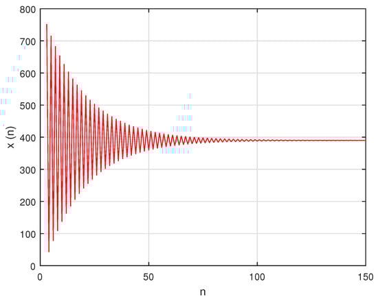
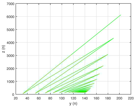
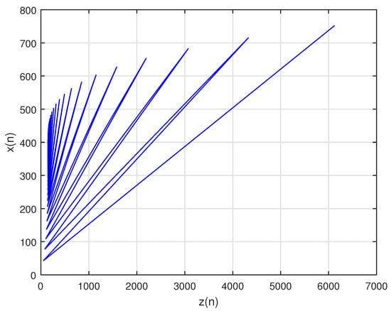
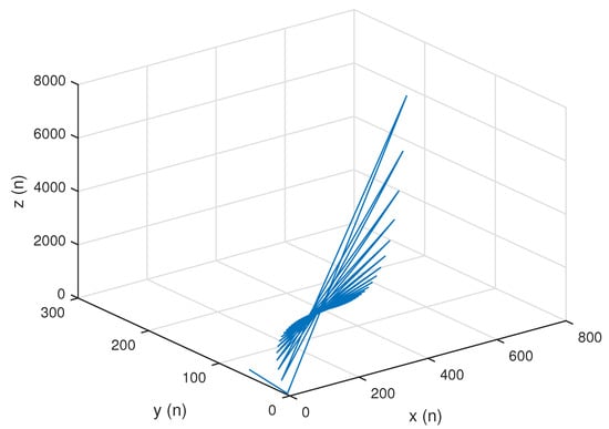
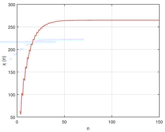
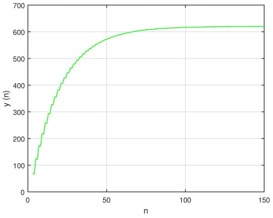
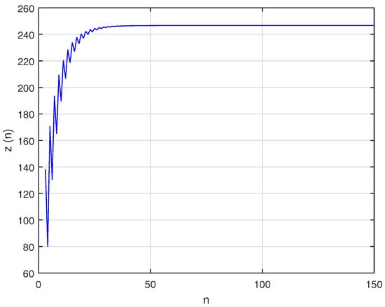
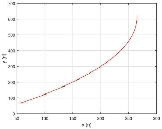
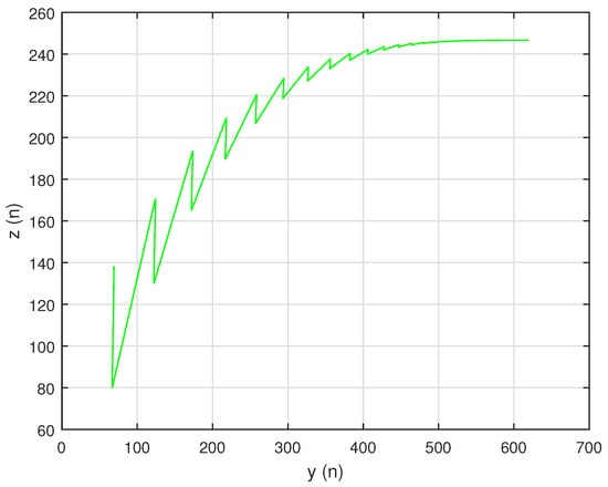
In this situation, the system’s unique positive equilibrium point $\left(57\right)$, is given by $(\overline{x},\overline{y},\overline{z})=(389.857,140.0,146.667).$ The graphs of $x_m,y_m$, and $z_m$are shown in Figure 1, Figure 2 and Figure 3, respectively, and $x_m{y}_m$, $y_m{z}_m$, and $z_m{x}_m$, the attractors of system $\left(57\right)$, are shown in Figure 4, Figure 5 and Figure 6, respectively. The graph of the phase portrait of system $\left(57\right)$ is also shown in Figure 7.

Figure 1. Graph of $x_m$ for system (57).

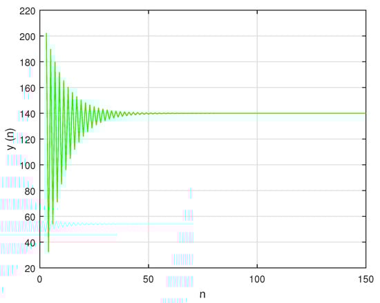
Figure 2. Graph of $y_m$ for system (57).

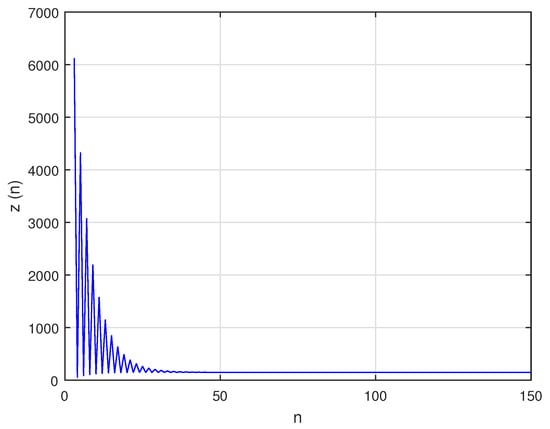
Figure 3. Graph of $z_m$ for system (57).

Figure 4. Attractor $x_m{y}_m$ for system (57).

Figure 5. Attractor $y_m{z}_m$ for system (57).

Figure 6. Attractor $z_m{x}_m$ for system (57).

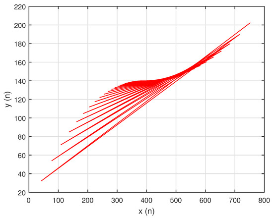
Figure 7. Phase portrait $x_m{y}_m{z}_m$ of system $\left(57\right)$.

Example 2. 

Let $A=53,B=0.8,C=532,\alpha =62,\beta =0.9,\gamma =834,\delta =74,\eta =0.7,\xi =736,$ for the sake of simplicity in the numerical figures, assume $U_m=x_m,V_m=y_m,W_m=z_m.$ Then, system $\left(1\right)$ becomes:

$$x_{m+1}=53+0.8x_{m-1}+532x_{m-1}{e}^{-y_m},y_{m+1}=62+0.9y_{m-1}+834y_{m-1}{e}^{-z_m}$$

$$z_{m+1}=74+0.7z_{m-1}+736z_{m-1}{e}^{-x_m}$$

(59)

with initial conditions $x_{-1}=2.8,x_0=3.7,y_{-1}=6.6,y_0=5.3,z_{-1}=3.4,z_0=8.5.$

In this situation, the system’s unique positive equilibrium point $\left(58\right)$, is given by $(\overline{x},\overline{y},\overline{z})=(265.0,619.773,246.667).$ The graphs of $x_m,y_m$, and $z_m$are shown in Figure 8, Figure 9 and Figure 10, respectively, and $x_m{y}_m$, $y_m{z}_m$, and $z_m{x}_m$, the attractors of system $\left(58\right)$ are shown in Figure 11, Figure 12 and Figure 13, respectively. The graph of the phase portrait of system $\left(58\right)$ is also shown in Figure 14.

Figure 8. Graph of $x_m$ for system (58).

Figure 9. Graph of $y_m$ for system (58).

Figure 10. Graph of $z_m$ for system (58).

Figure 11. Attractor $x_m{y}_m$ for system (58).

Figure 12. Attractor $y_m{z}_m$ for system (58).

Figure 13. Attractor $z_m{x}_m$ for system (58).

Figure 14. Phase portrait $x_m{y}_m{z}_m$ of system $\left(58\right)$.

Example 3. 

Let $A=35,B=0.7,C=5632,\alpha =82,\beta =0.8,\gamma =6634,\delta =44,\eta =0.9,\xi =7636.$ For simplicity, in numerical graphs we assume, $U_m=x_m,V_m=y_m,W_m=z_m$ Then, system $\left(1\right)$ can be written as:

$$x_{m+1}=35+0.7x_{m-1}+5632x_{m-1}{e}^{-y_m},y_{m+1}=82+0.8y_{m-1}+6634y_{m-1}{e}^{-z_m}$$

$$z_{m+1}=44+0.9z_{m-1}+7636z_{m-1}{e}^{-x_m}$$

(60)

with initial conditions $x_{-1}=2.8,x_0=3.7,y_{-1}=9.6,y_0=5.5,z_{-1}=4.4,z_0=8.3.$

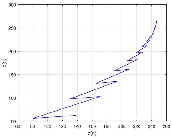
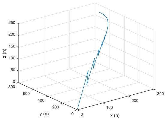
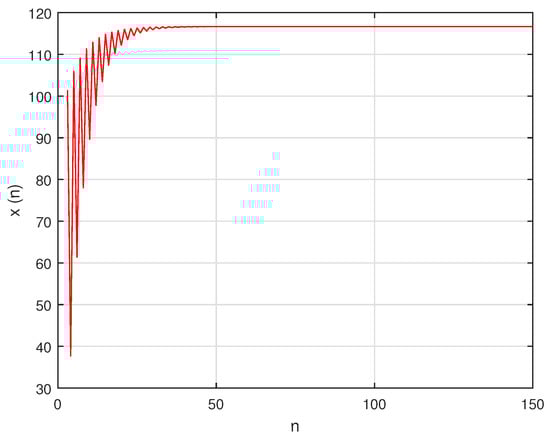
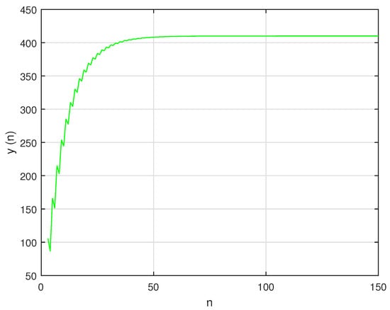
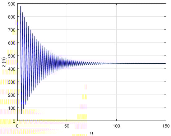
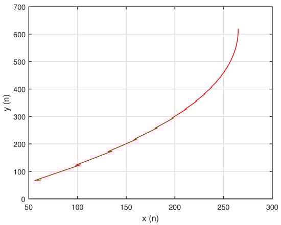
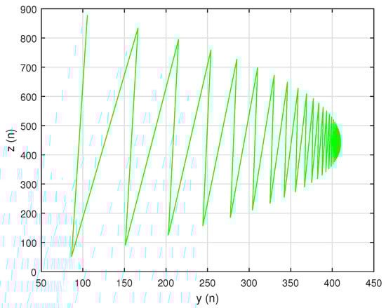
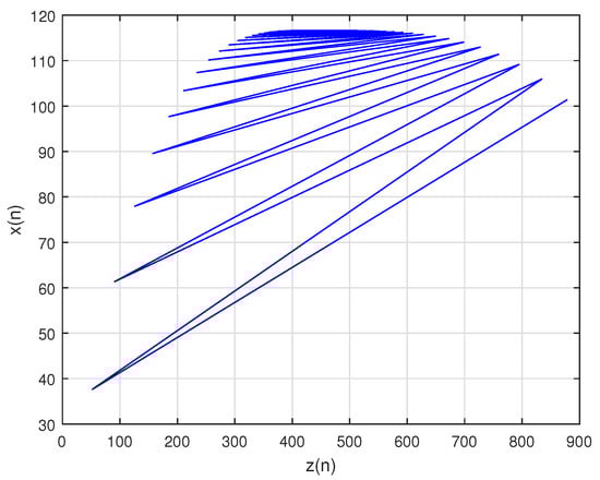
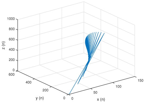
In this case, the unique positive equilibrium point of system $\left(59\right)$ is given by $(\overline{x},\overline{y},\overline{z})=(116.667,410.0,439.84).$ The graphs of $x_m,y_m$, and $z_m$are shown in Figure 15, Figure 16 and Figure 17, respectively, and $x_m{y}_m$, $y_m{z}_m$, and $z_m{x}_m$, the attractors of system $\left(59\right)$ are shown in Figure 18, Figure 19 and Figure 20, respectively. The graph of phase portrait of system $\left(59\right)$ is also shown in Figure 21.

Figure 15. Solution behavior of $x_m$ for system (59).

Figure 16. Solution behavior of $y_m$ for system (59).

Figure 17. Solution behavior of $z_m$ for system (59).

Figure 18. Attractor $x_m{y}_m$ for system (59).

Figure 19. Attractor $y_m{z}_m$ for system (59).

Figure 20. Attractor $z_m{y}_m$ for system (59).

Figure 21. Phase portrait $x_m{y}_m{z}_m$ of system $\left(59\right)$.

4. Conclusions

The qualitative behavior of a system of exponential difference equations is the subject of this paper. The asymptotic behavior of the solutions is obtained, with a necessary and sufficient condition, and presence and uniqueness of a positive fixed point of system $\left(1\right)$, having been investigated. The boundedness and persistence of the positive solutions have been demonstrated. Furthermore, we have demonstrated that the positive equilibrium point of system $\left(1\right)$, exists both locally and globally. In addition, the rate of convergence of the positive solutions of (1), converges to its positive equilibrium point. Finally, to enhance our theoretical discussion, a few numerical examples are provided.

References

- El-Metwally, H.; Grove, E.A.; Ladas, G.; Levins, R.; Radin, M. On the difference equation, Um+1 = α + βUm−1e−Um. Nonlinear Anal. 2001, 47, 4623–4634. [Google Scholar] [CrossRef]
- Papaschinopoluos, G.; Radin, M.A.; Schinas, C.J. On a system of two difference equations of exponential form: Um+1 = a + bUm−1e−Vm, Vm+1 = c + dVm−1e−Um. Math. Comput. Model. 2011, 54, 2969–2977. [Google Scholar] [CrossRef]
- Papaschinopoulos, G.; Schinas, C.J. On the dynamics of two exponential type systems of difference equations. Comp. Math. Appl. 2012, 64, 2326–2334. [Google Scholar] [CrossRef]
- Papaschinopoulos, G.; Radin, M.A.; Schinas, C.J. Study of the asymptotic behavior of the solutions of three systems of difference equations of exponential form. Appl. Math. Comp. 2012, 218, 5310–5318. [Google Scholar] [CrossRef]
- Gouasmia, M.; Ardjouni, A.; Djoudi, A. Study of asymptotic behavior of solutions of neutral mixed type difference equations. Open Jr. Math. Anal. 2020, 4, 11–19. [Google Scholar] [CrossRef]
- Iyanda, F.K. Algorithm analytic-numeric solution for nonlinear gas dynamic partial differential equation. Eng. Appl. Sci. Lett. 2022, 5, 32–40. [Google Scholar] [CrossRef]
- Al-Raeei, M. The study of human monkeypox disease in 2022 using the epidemic models: Herd immunity and the basic reproduction number case. Ann. Med. Surg. 2023, 85, 316–321. [Google Scholar] [CrossRef]
- Agarwal, R.P. Difference Equations and Inequalities, 2nd ed.; Dekker: New York, NY, USA, 2000. [Google Scholar]
- Elaydi, S. An Introduction to Difference Equations, 2nd ed.; Springer: Berlin/Heidelberg, Germany, 2005. [Google Scholar]
- Khaliq, A.; Ibrahim, T.F.; Alotaibi, A.M.; Shoaib, M.; El-Moneam, M.A. Dynamical Analysis of Discrete-Time Two-Predators One-Prey Lotka–Volterra Model. Mathematics 2022, 10, 4015. [Google Scholar] [CrossRef]
- Mazzia, F.; Trigiante, D. The role of difference equations in numerical analysis. Comput. Math. Appl. 1994, 28, 209–217. [Google Scholar] [CrossRef]
- Brenner, J.L.; D’Esopo, D.A.; Fowler, A.G. Difference Equations in Forecasting Formulas. In Management Science; Theory Series; Doubleday: New York, NY, USA, 1968; Volume 15, pp. 141–159. [Google Scholar]
- Frank, S.A. Control Theory Dynamics. In Control Theory Tutorial; Springer Briefs in Applied Sciences and Technology; Springer: Cham, Switzerland, 2018. [Google Scholar] [CrossRef]
- Chatzarakis, G.E.; Elabbasy, E.M.; Moaaz, O.; Mahjoub, H. Global Analysis and the Periodic Character of a Class of Difference Equations. Axioms 2019, 8, 131. [Google Scholar] [CrossRef]
- Khaliq, A.; Mustafa, I.; Ibrahim, T.F.; Osman, W.M.; Al-Sinan, B.R.; Dawood, A.A.; Juma, M.Y. Stability and Bifurcation Analysis of Fifth-Order Nonlinear Fractional Difference Equation. Fractal Fract. 2023, 7, 113. [Google Scholar] [CrossRef]
- Khaliq, A.; Alayachi, H.S.; Zubair, M.; Rohail, M.; Khan, A.Q. On stability analysis of a class of three-dimensional system of exponential difference equations. AIMS Math. 2023, 8, 5016–5035. [Google Scholar] [CrossRef]
- Khaliq, A.; Hassan, S.S. Analytical solution of a rational difference equation. Adv. Stud. Euro-Tbilisi Math. J. 2022, 15, 181–202. [Google Scholar] [CrossRef]
- Alotaibi, A.M.; Khaliq, A.; Ali, M.; Sadiq, S. On a Class of Discrete Max-Type Difference Equation Model of Order Four. Dis. Dyn. Nat. Soc. 2022, 2022, 8766711. [Google Scholar] [CrossRef]
- Grove, E.A.; Ladas, G.; Prokup, N.R.; Levis, R. On the global behavior of solutions of a biological modal. Commun. Appl. Nonlinear Anal. 2000, 7, 33–46. [Google Scholar]
- Papaschinopoulos, G.; Fotiades, N.; Schinas, C.J. On a system of difference equations including negative exponential terms. J. Differ. Equ. Appl. 2014, 20, 717–732. [Google Scholar] [CrossRef]
- Papaschinopoulos, G.; Ellina, G.; Papadopoulos, K.B. Asymptotic the behavior of the positive solutions of an exponential type system of difference equations. Appl. Math. Comput. 2014, 245, 181–190. [Google Scholar] [CrossRef]
- Phong, M.N. A note on a system of two nonlinear difference equations. Elect. Math. Anal. Appl. 2015, 3, 170–179. [Google Scholar]
- Zhang, D.C.; Shi, B. Oscillation and global asymptotic stability in a discrete epidemic model. J. Math. Anal. Appl. 2003, 278, 194–202. [Google Scholar] [CrossRef]
- Stefanidou, G.; Papaschinopoluos, G.; Schinas, C.J. On a system of two exponential type difference equations. Commum. Appl. Nonlinear Anal. 2010, 17, 1–13. [Google Scholar]
- Stević, S. On a discrete epidemic model. Discrete Dyn. Nat. Soc. 2007, 2007, 87519. [Google Scholar] [CrossRef]
- Grove, E.A.; Ladas, G. Periodicities in Nonlinear Difference Equations; Chapman and Hall/CRC: Boca Raton, FL, USA, 2005. [Google Scholar]
- Kocic, V.L.; Ladas, G. Global Behavior of Nonlinear Difference Equations of Higher Order with Applications; Kluwer Academic: Dordrecht, The Netherlands, 1993. [Google Scholar]
- Stević, S. On the recursive sequence . Indian J. Pure Appl. Math. 2002, 33, 1767–1774. [Google Scholar]
Disclaimer/Publisher’s Note: The statements, opinions and data contained in all publications are solely those of the individual author(s) and contributor(s) and not of MDPI and/or the editor(s). MDPI and/or the editor(s) disclaim responsibility for any injury to people or property resulting from any ideas, methods, instructions or products referred to in the content. |
© 2023 by the authors. Licensee MDPI, Basel, Switzerland. This article is an open access article distributed under the terms and conditions of the Creative Commons Attribution (CC BY) license (https://creativecommons.org/licenses/by/4.0/).