Research on Relative Threshold of Abnormal Travel in Subway Based on Bilateral Curve Fitting

Abstract

Abnormal passenger behavior in rail transit has become a top priority, as it affects operational safety. Passenger travel time is the main basis for identifying abnormal behavior while considering the flexibility of travel time. Currently, the main method is to use absolute threshold discrimination based on the distribution of travel time. However, there is a problem of missing abnormal passenger behavior due to the large difference in travel time between the Origin-Destinations (ODs). Therefore, this paper proposes a method of setting corresponding thresholds for each OD. By analyzing the percentile curves of the overall and individual OD pairs, it was found that the turning point of the curve had a significant feature, and the difference between the two sides of the curve was obvious. This paper proposes a bilateral fitting method, and the results show that this method can calculate the relative threshold for different OD pairs. The significant advantages of this method are its low cost and wide coverage.

1. Introduction

In recent years, China’s urban rail transit has developed rapidly, with the scale of the network and passenger flow ranking first in the world and reaching 9206.8 km and 23.69 billion passenger trips, respectively, in 2021 [1]. In 2020, 5 cities in mainland China ranked in the top 10 of the world’s urban subway passenger flow among 137 cities in 46 countries [2]. The vast network and passenger flow make the daily risk control of urban rail transit increasingly severe. At the same time, incidents such as begging, selling, promoting, and theft still occur, seriously affecting the safety of the urban rail transit system and becoming the main source of risk. Therefore, the identification of abnormal passenger behavior in urban rail transit has become an important task for its safe operation management.

Many scholars are researching abnormal passenger behavior. Pan et al. [3] detected anomalies through human movement data and social media data. Zhao et al. [4] analyzed passenger travel patterns from the perspectives of time, space, and spatiotemporal factors to understand hidden patterns and anomalies in travel patterns. Wang [5] deeply explored the travel patterns of abnormal rail transit passengers based on Beijing’s rail transit card data, extracted passenger travel pattern features, and identified abnormal travel passengers. Zhao [6] combined long-term intelligent card transaction data of passengers to deeply understand and explore their travel models and then conducted in-depth analysis of the aspects of discovered patterns and detected anomalies in passenger travel patterns by using statistical methods to analyze the distribution characteristics of passenger travel patterns and anomalies in travel time and space for abnormal passengers.

Currently, the main method used in the identification of abnormal passenger behavior is the absolute threshold method, which ignores the huge differences between different Origin-Destinations (ODs) and can easily lead to omissions in identifying abnormal passenger behavior. Liu [7] analyzed the abnormal behavior of typical card numbers in Beijing’s rail transit OD (Origin-Destination) data and classified them into three categories. The method of judging abnormal behavior using a fixed threshold was used. Xue [8] and others analyzed long-term stationary passengers based on fixed time using the AFC system in the subway in 2019. Yu [9] and others analyzed passenger long- and short-term records based on fixed threshold using passenger OD data in the subway AFC system.

To study the critical values considering different factors, Li et al. [10] proposed the concept of the relative threshold index in their research on extreme temperature events. Ouyang [11] used quantiles to analyze indicator risk. There are two main types of threshold-selection methods: qualitative and quantitative. Han [12] analyzed the trends of extreme high and low temperatures and extreme precipitation in Southern Xinjiang over the past 51 years using the percentile threshold method and studied their impact on agricultural production. Wang [13] used the percentile method to determine the spatial distribution of hourly extreme precipitation thresholds and considered the corresponding thresholds for national stations and recurrence periods.

Libardo et al. [14] analyzed the percentage changes in transportation demand generated by fluctuations in GDP per unit in the Italian region as the main object and used this to make predictions as well as to deduce the relationship between transportation demand and GDP. Rich et al. [15] believed that long-distance travel is becoming increasingly important and estimated different types of tourism elasticity based on travel data, taking into account factors such as travel distance and purpose.

The quantitative method mainly selects the optimal threshold by analyzing one-sided data. Neil [16] used a parameter curve fitting method to analyze the tail of the distribution and study the pricing of high excess losses in insurance. Goegebeur [17] and others determined the optimal threshold by analyzing the tail index of the curve. However, only considering one-sided data can lead to biased high or low threshold values. Considering the limitations of the one-sided curve, Tang [18] designed a segmented curve for the special saddle-shaped performance curve of the water pump when studying the performance of the water pump and used the least squares polynomial to fit the designed segmented curve. Chen [19] made a logistic curve of the urbanization level, which is divided into three stages: the initial stage, the rapid stage, and the saturation stage. Duan [20] proposed a curve segmentation method weighted by the starting point, which has small fitting errors and is easy to program. In terms of transportation quality evaluation, Nocera [21,22] emphasized the importance of passenger travel quality, providing assistance for policy makers to make wise judgments for future plans. Additionally, Nocera, S. proposed practical methods for quality evaluation.

Through the analysis of research literature, it was found that the attention paid to abnormal passenger behavior in the time characteristics of passengers is not high enough, the analysis is not detailed enough, and the method is too simple and lacks pertinence and cannot effectively identify abnormal time, which can lead to a lot of abnormal passenger behavior being missed. The existing threshold determination methods in various fields are mainly divided into qualitative and quantitative methods. Qualitative methods determine thresholds through observation and experience, which are subjective and have varying results and poor stability. Quantitative methods directly use formulas to calculate or determine thresholds based on one-sided tail data distribution.

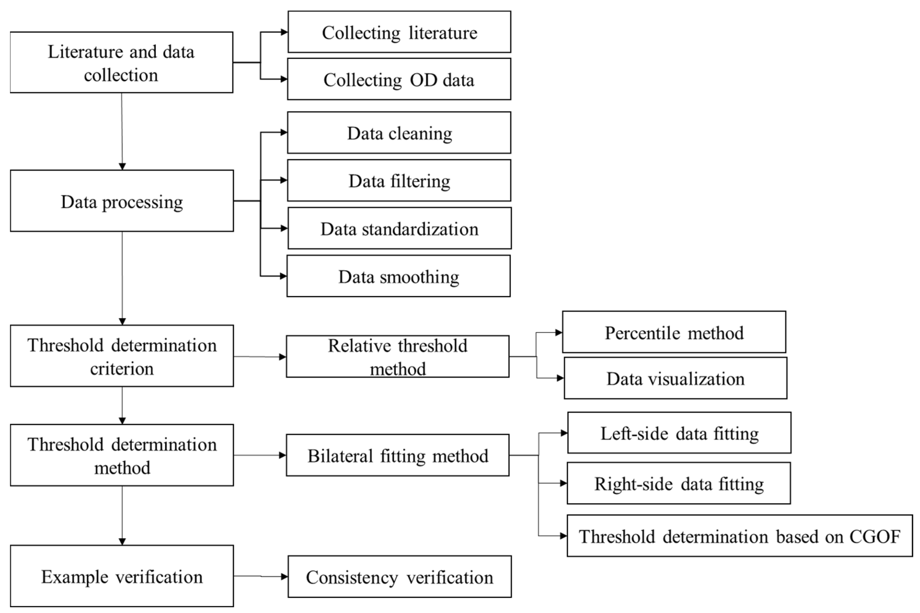
This paper considers the travel time distribution of different ODs and uses relative thresholds for discrimination. Based on the current quantitative research, due to the significant difference in distribution characteristics on both sides of the quantile curve, a bilateral fitting method [23,24,25,26,27] is proposed for threshold determination. Figure 1 is used to present the overall technical research plan roadmap. The specific content includes the following:

(1) Based on OD data, analyze passenger travel time. Preprocess the OD data and calculate the travel time of passengers and analyze the proportion of abnormal passenger behavior in terms of time and space dimensions under the absolute threshold.

(2) Taking into account the travel time distribution of different ODs, relative threshold is used as the discrimination criterion. The distribution characteristics of the average travel time of OD individuals and the total population are analyzed, and the characteristics of curve mutation are extracted. The mutation range is analyzed, and the idea of using relative thresholds as the determination standard is proposed.

(3) This paragraph describes the method for calculating the relative threshold based on the double-sided fitting approach. First, the left and right sides of the curve data are separately fitted to determine the single OD threshold based on comprehensive fitting goodness. Then, the average percentile method is used to determine the relative threshold for multiple ODs.

(4) Case analysis and validation. After visualization, the effect of bilateral fitting is obtained, and the relative threshold values for multiple ODs are calculated and analyzed. The consistency of the threshold quantile results for different ODs is tested to verify the rationality and effectiveness of the method.

2. Travel Time Analysis

2.1. Data Preparation

Due to the significant passenger traffic volume on Guangzhou Metro and our collaborative partnership with the company, we were able to access relevant data. Therefore, this paper selects Guangzhou Metro as the research object. As of 2021, there are 24 subway lines and 411 operating stations in Guangzhou Metro with a network length of 744.5 km.

This paper selected the passenger swipe card data from 27 days in 2018 for the study, which includes over 30 million swipe records. Each passenger’s swipe record contains 13 attributes, such as user card number, recharge time, balance, entry/exit station time, entry/exit station line, and entry/exit station name, and fully records the passenger’s entry/exit time and location information. In order to facilitate data processing and meet the requirements of the study, this paper selected 7 relevant attributes from the 13 attributes for processing, including user card number, entry station, exit station, entry time, exit time, entry station line, and exit station line.

The original data contains some useless data that may affect the analysis, such as records where the entry time and exit time are the same due to system errors and records of excessively long travel time that violate the subway travel requirements. Therefore, this paper preprocesses the original data by removing useless and erroneous information to ensure more accurate analysis of travel data. The main steps are as follows:

(1) Trip duration calculation. Trip duration refers to the time that passengers spend riding on the rail transit, which is determined based on the time when passengers swipe their card to enter and exit the station. In order to conduct more precise research, the unit of time measurement is in seconds.

(2) Deleting erroneous data. There is a large amount of data in the original passenger card-swiping records where the entry time is equal to the exit time, which does not comply with the general rules of taking a ride. Therefore, this part of the data was deleted.

(3) Determining passenger travel peak periods. In this paper, travel between 7:30 a.m. and 9:30 a.m. is referred to as the morning rush hour, and travel between 5:30 p.m. and 7:30 p.m. is referred to as the evening rush hour. Travel during other times is referred to as off-peak travel.

(4) Standardization. Due to the large differences in distances and number of stations between OD pairs, data standardization is the transformation of different OD trip time data into standardized time data.

2.1.1. Absolute Threshold Index of Travel Time

In this paper, the abnormal behavior in subways is identified based on the travel time, and the threshold value is the most important for determining the abnormal behavior of passengers. In consideration of the provisions of Guangzhou Metro Company, in this paper 270 min is taken as the critical value to judge the abnormal behavior of passengers, and this method using a fixed value as the critical value is called the absolute threshold method. The abnormal behavior under absolute threshold is analyzed from two dimensions of space and time.

2.1.2. Analysis of Abnormal Behavior Based on Spatial Dimension

(1) Spatial dimension indicator determination

The number of OD station spacing is selected as a spatial index for analysis. OD station number can reflect the travel distance of passengers in space.

(2) Analysis of the anomaly ratio considering the number of interval stations

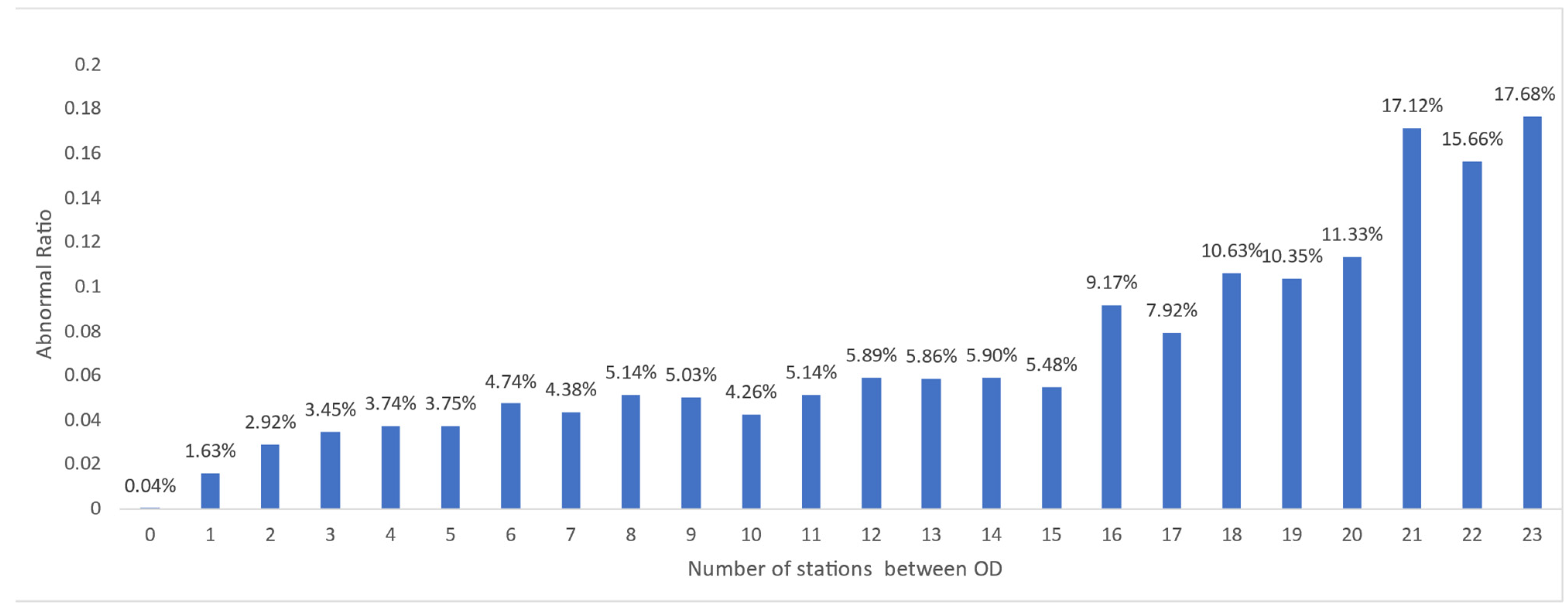
The proportion of abnormal behavior of OD with different number of interval stations is analyzed as shown in Figure 2 and is represented by a bar chart. The abscissa represents the number of interval stations between OD, and the ordinate represents the abnormal proportion.

As can be seen in Figure 2, the proportion of abnormal behavior of passengers varies with the number of OD interval stations, showing an overall increasing trend. When the number of OD interval stations is between 1 and 15, the proportion of abnormal behavior is between 2% and 6%. When the number of interval stations is between 16 and 23, the proportion of abnormal behavior is generally high, between 8% and 18%.

Under the absolute threshold, the number of different sites in the spatial dimension has a significant impact on the proportion of anomalies. Generally, as the number of sites increases, the proportion of anomalies gradually increases. This is because when setting the threshold, passengers with longer travel times due to more sites are taken into consideration, and therefore the threshold is set higher, with abnormal behavior mainly concentrated in ODs with more sites. On the other hand, when the number of sites is small, the proportion of anomalies is relatively low. This is because setting the threshold too high makes it more difficult to detect abnormal passenger behavior and also because the differences in passenger behavior over a short period of time are small, making abnormal behavior easy to ignore. Based on the above analysis, we need to consider different numbers of sites to set different thresholds.

2.1.3. Analysis of Abnormal Behavior Based on the Time Dimension

(1) Time dimension indicator determination

The time is divided into three parts: morning peak time, evening peak time, and off-peak time. The morning peak time is from 7:30 to 9:30, the evening peak time is from 17:30 to 19:30, and the other subway operation time is off-peak time.

(2) Analysis of the anomaly ratio considering the peak period

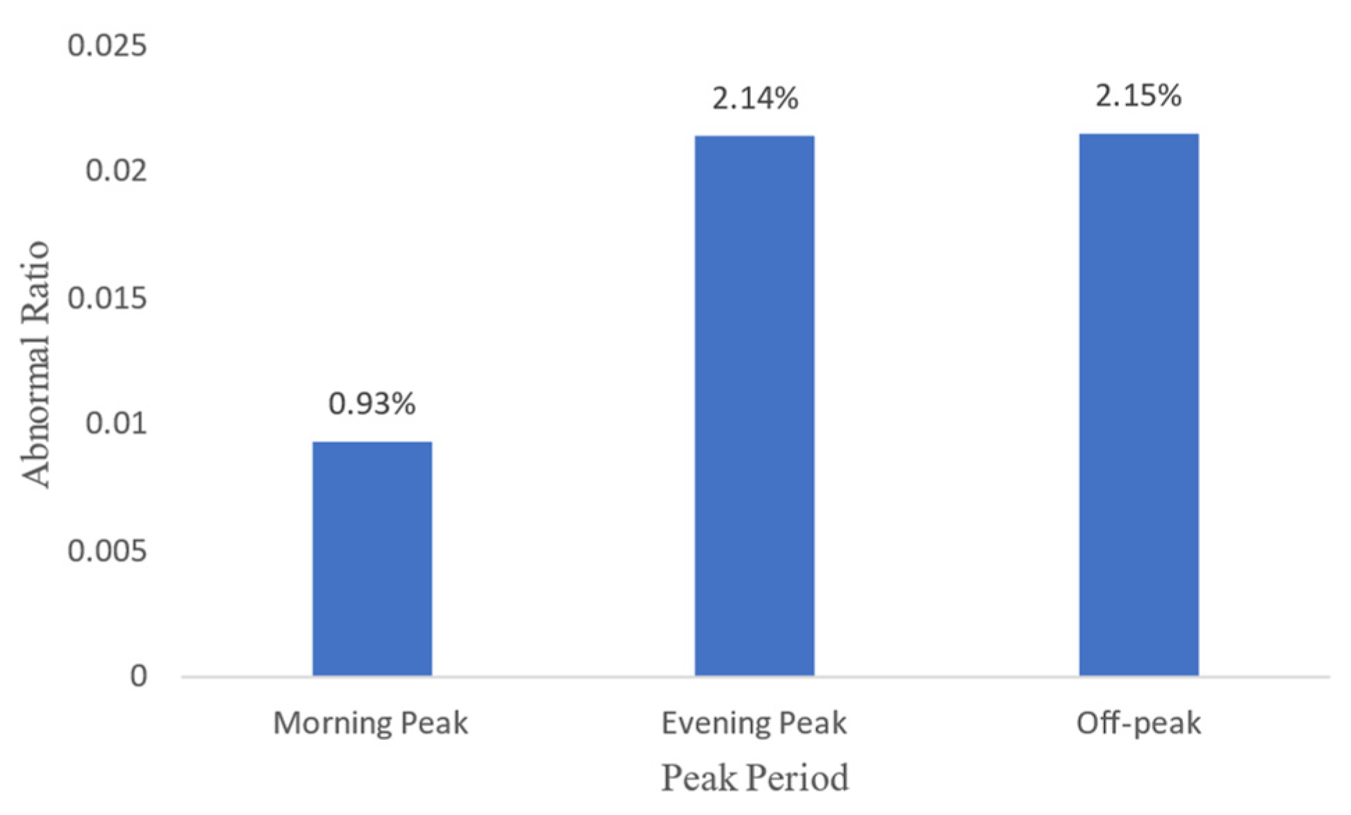
The proportion of abnormal behavior in different peak periods is analyzed as shown in Figure 3 and is represented by a bar chart. The abscissa represents different peak periods (morning peak, and evening peak, and off-peak, respectively), and the ordinate represents the proportion of abnormal behavior.

As can be seen in Figure 3, the proportion of abnormal behavior of passengers varies with the peak period. The proportion of abnormal behavior in morning-peak, evening peak, and off-peak periods are 0.93%, 2.14%, and 2.15%, respectively.

In addition, it can be seen in Figure 3 that different peak periods of time dimension also have significant influences on the proportion of anomalies. We need to set different thresholds according to different peak periods.

3. Travel Time Distribution Characteristics

3.1. Analytical Method

The sample size of travel time data is uneven. The sample size of different OD data sets is different. The minimum sample size is 1205, and the maximum sample size can reach 24,539.

Distributed analysis method. In this paper, the Quantile groups method [28] is adopted to model the travel time and analyze its distribution characteristics. The quantile accuracy is 1/1000. This method can eliminate the unbalance of sample size.

3.2. Overall Distribution Characteristics

3.2.1. Overall Data Construction

The population refers to all OD, and the average quantile method is adopted when studying the time distribution characteristics of the population. The calculation steps of the average quantile method are as follows: first, the combination of thousandths of each OD is calculated, and then the average value of different quantiles is calculated.

3.2.2. Analysis of the Overall Distribution Characteristics

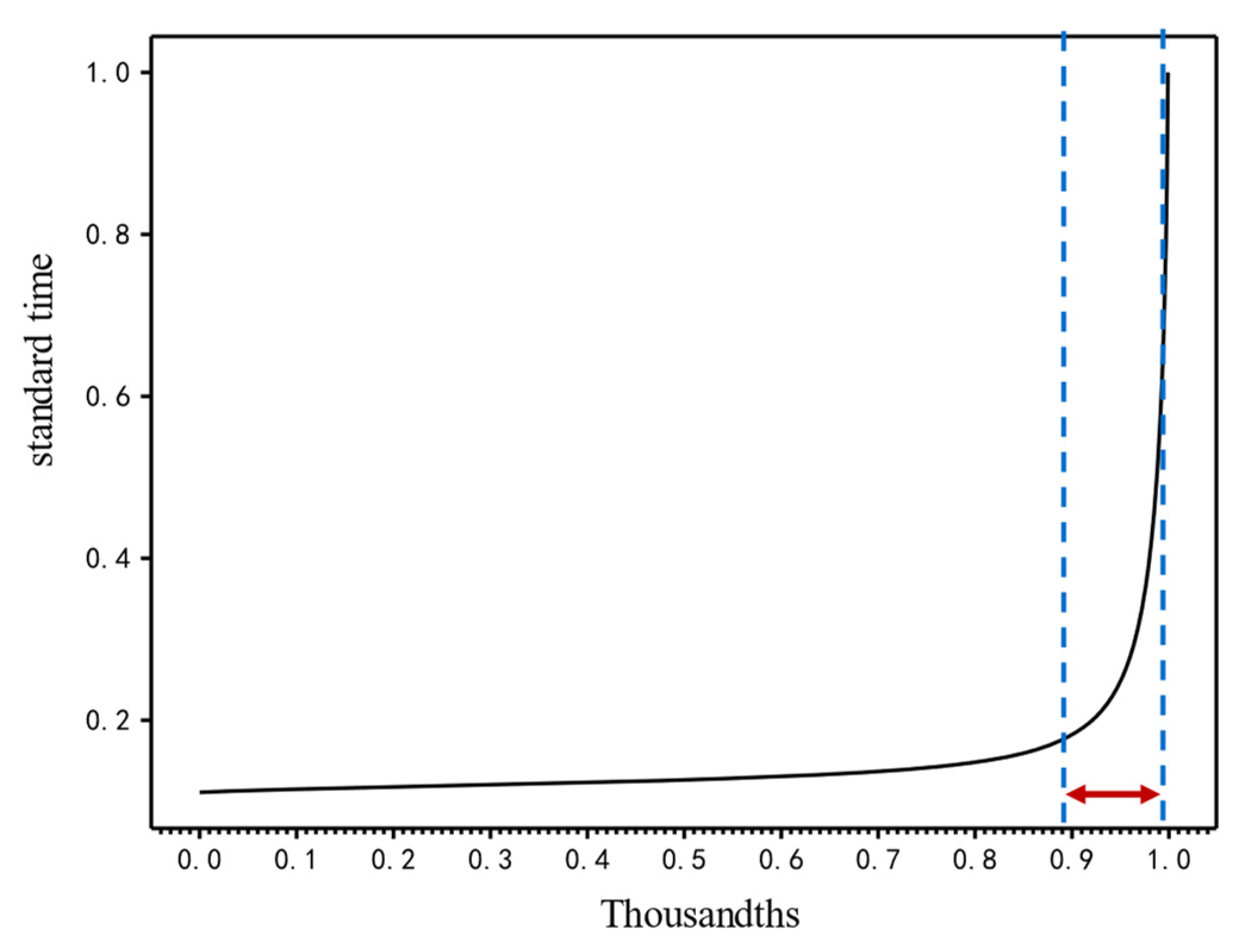
Graph of population mean quantile. As shown in Figure 4, abscissa represents quantile, and ordinate represents standard time. As can be seen in Figure 4, the curve presents three stages: steady rising stage, fast rising stage, and rapid rising stage. The steady rise stage of the curve is between the quantiles 0 and 0.9, and within this range the data fluctuation is small, and the slope of the curve is small and gentle. The stage of rapid rise and rapid rise is between 0.9 and 1.

Extraction of mutation characteristics. As can be seen in Figure 4, the overall distribution curve has undergone sudden changes, and the curves on both sides of the mutation point are significantly different, with a mutation range of 0.9–1.

3.3. OD Distribution Characteristics

3.3.1. OD Sampling Design

(1) Filter based on the number of spaced sites. (1) The number of interval stations is divided into four groups: [0, 8), [8, 16), [16, 24), [24, 33]. (2) The OD group is divided according to the number of interval stations.

(2) Select according to the data amount. (1) Calculate the data amount of each OD. (2) Calculate the average data amount of each group. (3) Select the OD whose data amount is equal to or closest to the average data amount of the group, called the average OD. (4) If there is only one average OD, select the OD; if there are multiple ODs, select the method of random extraction.

3.3.2. Analysis of the Distribution Characteristics of the Sampled OD

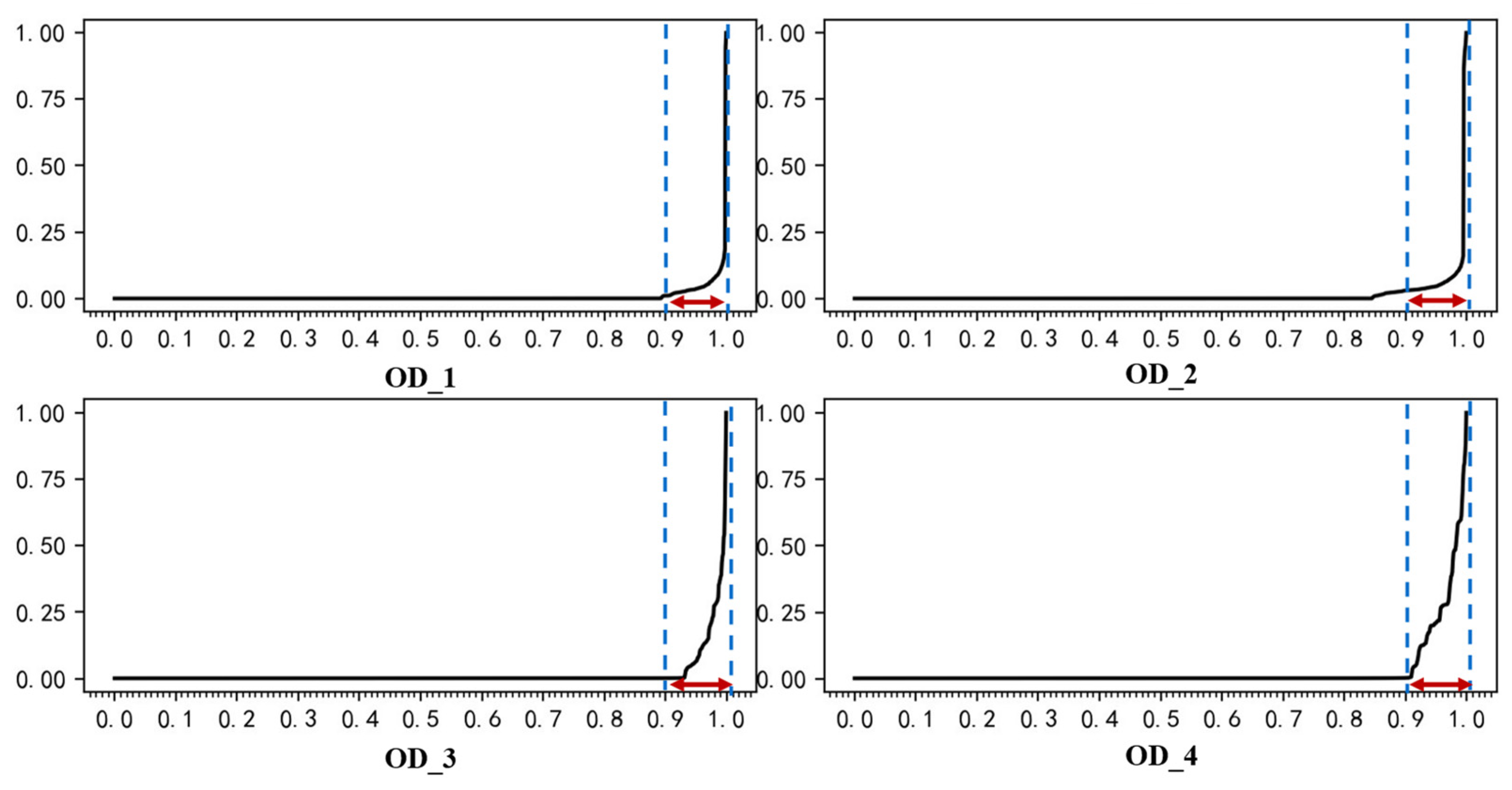
The travel time distribution diagram of sampling OD is shown in Figure 5. In Figure 5, the abscissa represents quantile, and the ordinate represents standard time. The standard time distribution of four samples of OD was analyzed, and the transverse comparison showed that the curves of four samples of OD were similar in shape. All show an increasing trend. In longitudinal analysis, the curve is consistent with the population and also presents three stages, and the range of different stages is similar to the population.

The travel time distribution diagram of sampling OD is shown in Figure 5. In Figure 5, the abscissa represents thousandths, and the ordinate represents standard time. The standard time distribution of four samples of OD was analyzed, and the transverse comparison showed that the curves of four samples of OD were similar in shape. All show an increasing trend. In longitudinal analysis, the curve is consistent with the population and also presents three stages, and the range of different stages is similar to the population.

Extraction of mutation characteristics. Abrupt changes in standard times were observed in all four ODs, and the mutation range was consistent, 0.9–1.

3.4. Relative Threshold Thought

The meaning of relative threshold. The relative threshold sets different quantiles for different ODs, considering the difference in distance and number of stations between incoming and outgoing stations and threshold discrimination based on quantiles from the perspective of probability.

The relative threshold is feasible. No matter what the overall or individual trend of OD is, the standard time distribution curve is similar in shape, mutation occurs in all cases, and the consistency is strong in the mutation range. Therefore, the relative threshold is feasible.

Advantages over thresholds. Compared with the absolute threshold, the relative threshold can adjust the threshold of abnormal behavior according to different ODs so that the abnormal behavior can be detected more accurately. Due to the huge differences between different OD, the setting of absolute threshold is difficult to adapt to all cases. The relative threshold can be adjusted according to OD differences to improve the accuracy of anomaly detection.

4. Relative Threshold Projection Based on Change Points

According to the characteristics of abrupt points and bilateral curve distribution, a two-sided fitting method was proposed to determine the time threshold of single ODs. In addition, considering the threshold of all ODs, the relative threshold is determined by means of average thousandth place method.

4.1. Single Change Point Threshold Determination

4.1.1. Change Point

The change point is the intersection of two adjacent sections of a curve, that is, the point at which one section of the curve changes to another. It can be seen in Section 3 that there are obvious sudden changes in the quantile, and there are obvious differences between the left curve and the right curve. There are change points in the middle of the left curve and the right curve. The abrupt change range of quantile curve is 0.9–1, so the selection range of change point is 0.9–1.

4.1.2. Bilateral Fitting Method

(1) Curve division. As can be seen in Section 3, the quantile curve has obvious change points, and the slope of curves on both sides is very different. Therefore, the curve is divided into two sections, the left side and the right side.

(2) The fitting method. The shape of the quantile curve of the population and individual is similar to that of the exponential function. The curve of the exponential function model is smooth and meets the monotonicity requirement of the quantile curve to the fitting function. The exponential function model of the fitting curve is defined by Equation (1):

$$\mathrm{y} = \mathrm{a}\times {\mathrm{e}}^{\mathrm{b}\times \mathrm{x}},$$

(1)

where a, b is the parameter and e is the base number.

(3) Piecewise curve-fitting. The least square method was used to fit the curves on the left and right sides. The least square method is a commonly used parameter determination method. It obtains the fitting parameter by minimizing the sum of the squares of error between the predicted value and the actual value.

(4) Goodness of fit evaluation. The determination coefficient is used to measure the fitting effect of the curve. Its value can directly reflect the degree of fit between the estimated value of the trend line and the corresponding actual data. The higher the degree of fit, the higher the reliability.

(5) Sectional evaluation. The determination coefficients of the left and right curves are calculated separately.

4.1.3. Threshold Determination

Threshold determination statistics. In this paper, the statistic CGOF is used as the index to determine the threshold. CGOF stands for “comprehensive goodness of fit.” CGOF is a statistic to determine the optimal threshold by combining the left and right curve fitting effects. Equation (2) defines CGOF:

$$\mathrm{CGOF} =\left|{\mathrm{R}}_{\mathrm{l}}^2+{\mathrm{R}}_{\mathrm{r}}^2-2\right|,$$

(2)

where, ${\mathrm{R}}_{\mathrm{l}}^2$ represents the determination coefficient of the left curve and ${\mathrm{R}}_{\mathrm{r}}^2$ represents the determination coefficient of the right curve. In this paper, the optimal threshold based on asymptotic CGOF minimum is deduced from the fitting angle.

4.2. Multivariate Change Point Relative to Threshold Determination

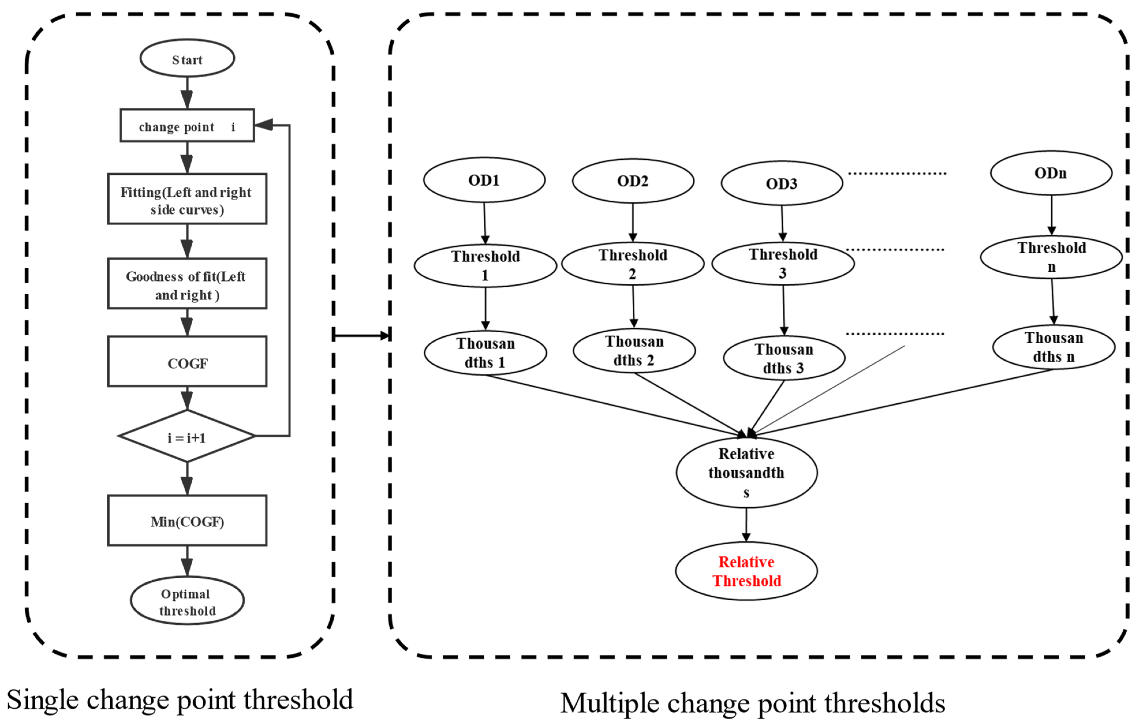
The relative threshold is determined using the mean kilobit method, which first calculates the variable point threshold based on the two-sided fitting method, and then calculates the average thousandth of all ODs and later determines the relative threshold considering the travel time of individual ODs. Figure 6 shows the flow chart of relative threshold derivation.

5. Example Verification

5.1. Example Analysis

5.1.1. Bilateral Fitting Results

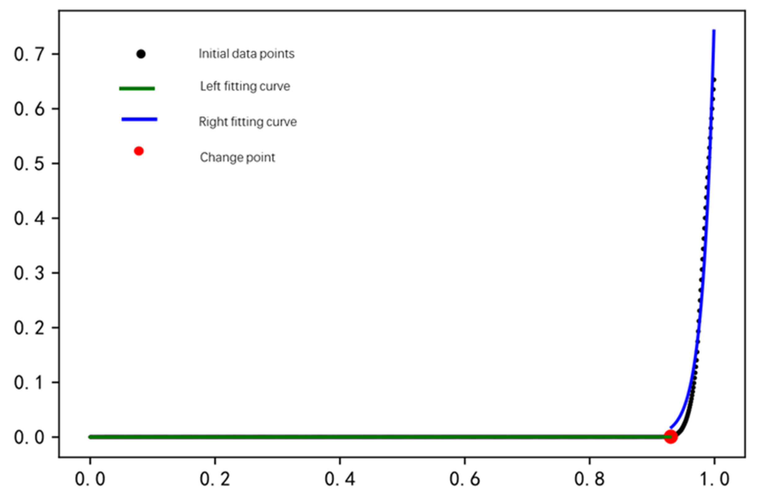
Figure 7 shows the bilaterally fitted effect of one of the ODs. The green curve in Figure 7 indicates the fit to the left data points, the blue curve indicates the fit to the right data points, and the red points indicate the change points from which it can be seen that the exponential function fits well to the left and right data points and that the change points are positioned between the curves.

5.1.2. Relative Threshold

As shown in

Table 1. Relative thresholds of ODs.

OD Code	OD1	OD2	OD3	OD4	OD5	OD6	OD7	OD8
Relative threshold	827	700	1831	678	739	573	818	1000
Abnormal criteria	13.78	11.67	30.52	11.30	12.32	9.54	13.63	16.67

, the relative thresholds of some ODs are demonstrated. It can be seen in Table 1 that different ODs have different thresholds and that different ODs have different standards for abnormal passenger behavior. The minimum is 9.53 min, and the maximum is 30.52 min.

5.2. Consistency Verification

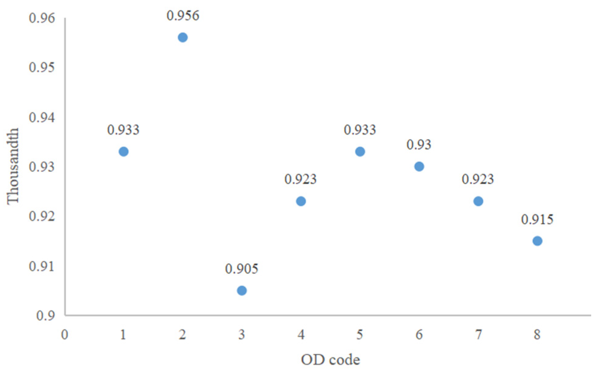
A total of 8 sets of OD data are calibrated. Each set of OD data is given an initial thousandth, and the consistency test of relative threshold is to check the consistency of the initial thousandth of each OD. As seen in Figure 8, there are two data points with large deviations, and then the 8-quantile variance is calculated with a value of 2 parts per thousand, so the deviation is not significant, and the bilateral fitting method has reasonableness and validity.

6. Research Conclusions and Outlook

6.1. Research Conclusions

In this paper, in order to analyze the influence of absolute threshold on the discrimination of passengers’ abnormal behavior, fixed values were used as thresholds to study the proportion of passengers’ abnormal behavior in two dimensions: spatial and temporal. It was found that in both dimensions, the number of different stations and peak periods have significant effects on the proportion of abnormal behavior, and the results of the study imply that absolute threshold cannot adequately identify abnormal behavior when passengers travel with large spatial and temporal differences.

In order to propose a more effective method for discriminating abnormal behavior, this paper analyzed the trends of OD overall and individual quantile curves, and the study found that the distribution curves were similar in shape. Both mutations occurred, both were consistent in the mutation range, and the idea of relative thresholds was proposed.

The distribution characteristics of quantile curves were studied, and it was found that the curve mutations had obvious mutations and large differences between the curves on both sides of the mutations. In this paper, a bilateral fitting method was proposed, and the relative threshold values were determined by combining the average thousandth quantile. It was found that the method can calculate the relative thresholds for different ODs. Different ODs have different thresholds and different criteria for abnormal passenger behavior.

The threshold quantile reflects the proportion of abnormal passenger behavior in different ODs, and the proportion of abnormal passenger behavior seriously affects the quality of rail transit. The calculated threshold quantile mean for multiple ODs is 92.69%, which means that 7.31% of passenger behavior in rail transit is abnormal. This proportion is high, indicating low passenger service quality and generally poor transportation quality.

Compared to previous research, the relative threshold method is better suited for situations where there are significant spatiotemporal differences in passenger travel behavior, as it can calculate relative thresholds for different origin-destination pairs. This allows for different standards of abnormal behavior and better adaptation to different OD situations, improving the accuracy of anomaly detection. The bilateral fitting method, based on the analysis of right-tail data and the consideration of normal data distribution, enhances the stability and accuracy of threshold determination.

6.2. Outlook

In this paper, when using the bilateral fitting method to determine the threshold, the fitting method is the exponential function, the parameter determination method is least squares, and the index to evaluate the fitting effect is the coefficient of determination, which can be optimized in three aspects of the fitting model, the parameter determination method, and other methods in future research to improve the fitting effect and the accuracy of threshold determination.

References

1. CAMET. Annual Statistics and Analysis Report on Urban Rail Transit in 2021. Urban Rail Transit. 2022, 77, 10–15. [Google Scholar]
2. Han, B.; Yang, Z.; Yu, Y.; Qian, L.; Chen, J.; Ran, J.; Qian, L.; Sun, Y.J.; Yu, Y.R.; Xi, Z.; et al. Overview of Statistics and Analysis of Urban Rail Transit Operations in the World in 2020. Urban Rapid Rail Transit. 2021, 34, 5–11. [Google Scholar]
3. Pan, B.; Zheng, Y.; Wilkie, D.; Shahabi, C. Crowd Sensing of Traffic Anomalies Based on Human Mobility and Social Media. In Proceedings of the 21st ACM SIGSPATIAL International Conference on Advances in Geographic Information Systems, Orlando, FL, USA, 5–8 November 2013; pp. 344–353. [Google Scholar]
4. Zhao, J.; Qu, Q.; Zhang, F.; Xu, C.; Liu, S. Spatio-temporal analysis of passenger travel patterns in massive smart card data. IEEE Transp. Intell. Transp. 2017, 18, 3135–3146. [Google Scholar] [CrossRef]
5. Wang, L. Research on Screening and Visualization Methods of Abnormal Passengers in Rail Transit. Master’s Thesis, Beijing University of Technology, Beijing, China, 2017. [Google Scholar]
6. Zhao, J.J. Urban Rail Transit Passenger Space-Time Travel Pattern Mining and Dynamic Passenger Flow Analysis. Ph.D. Thesis, University of Chinese Academy of Sciences, Beijing, China, 2017. [Google Scholar]
7. Liu, Z.L. Study on Passenger Travel Characteristics and Abnormal Behavior of Beijing Urban Rail Transit from the perspective of Same Station Entry and Exit. Ph.D. Thesis, Beijing Jiaotong University, Beijing, China, 2020. [Google Scholar]
8. Xue, G.; Gong, D.; Zhang, J.; Zhang, P.; Tai, Q. Passenger Travel Patterns and Behavior Analysis of Long-Term Staying in Subway System by Massive Smart Card Data. Energies 2020, 13, 2670. [Google Scholar] [CrossRef]
9. Yu, W.; Bai, H.; Chen, J.; Yan, X. Anomaly detection of passenger OD on Nanjing metro based on smart card big data. IEEE Access 2019, 7, 138624–138636. [Google Scholar] [CrossRef]
10. Li, Y.J.; Ren, G.Y.; Zhan, Y.J. A brief discussion on the threshold determination method in the study of extreme temperature events. Meteorol. Sci. Technol. Prog. 2013, 3, 36–40. [Google Scholar]
11. Ouyang, Z.S.; Zhou, X.W. The spillover effect of systemic financial risk on macroeconomy: Based on quantile to quantile method. Stat. Res. 2022, 39, 68–83. [Google Scholar]
12. Han, H.M.; Li, Q. Extreme climate change in Southern Xinjiang and its impact on agricultural production: A study based on the percentile threshold method. Hubei Agric. Sci. 2014, 53, 1801–1805. [Google Scholar]
13. Wang, Z.Q.; Xue, Y.J.; Huang, J.Y. Study on the distribution of hourly extreme precipitation thresholds and recurrence periods in Jinhua City. Zhejiang Meteorol. Serv. 2022, 43, 41–44+49. [Google Scholar]
14. Libardo, A.; Nocera, S. Transportation Elasticity for the Analysis of Italian Transportation Demand on a Regional Scale. Traffic Eng. Control 2008, 49, 187–192. [Google Scholar]
15. Mabit, S.L.; Rich, J. A long-distance travel demand model for Europe. Eur. J. Transp. Infrastruct. Res. 2011, 12, 1–20. [Google Scholar]
16. McNeil, A.J. Estimating the tails of loss severity distributions using extreme value theory. Astin Bull. 1997, 27, 117–137. [Google Scholar] [CrossRef] [Green Version]
17. Goegebeur, Y.; Beirlant, J.; de Wet, T. Linking Pareto-tail kernel goodness-offit statistics with tail index at optimal threshold and second order estimation. REVSTAT Stat. J. 2008, 6, 51–69. [Google Scholar]
18. Tang, L.D.; Xiao, M.; Tang, Y. Segmented Least Squares Polynomial Fitting Algorithm for Pump Performance Test Curve. J. Drain. Irrig. Mach. Eng. 2017, 35, 744–748. [Google Scholar]
19. Chen, Y.G. Types, segments and research methods of urbanization level growth curves. Sci. Geogr. Sin. 2012, 32, 12–17. [Google Scholar]
20. Wang, N.; Zhao, W.H.; Duan, Z.Y. A First-Order Continuous Segmented Curve Fitting Method. Modul. Mach. Tool Autom. Manuf. Tech. 2016, 507, 29–31+35. [Google Scholar]
21. Nocera, S. The key role of quality assessment in public transport policy. Traffic Eng. Control 2011, 52, 394–398. [Google Scholar]
22. Nocera, S. An Operational Approach for Quality Evaluation in Public Transport Services. Ing. Ferrov. 2010, 65, 363–383. [Google Scholar]
23. Liu, S.C. Subsection fitting and prediction of China’s urbanization level growth curve. Stat. Theory Pract. 2022, 18–22+31. [Google Scholar]
24. Liu, G.H. Characteristic curve fitting method of flexible piezoresistive pulse sensor. Transducer Microsyst. Technol. 2021, 40, 27–29+33. [Google Scholar]
25. Zhang, Y.X. The smooth method of piecewise function and its application in curve fitting. J. Southwest Univ. Natl. 2007, 486–490. [Google Scholar]
26. Hou, C.J. Globally continuous piecewise least squares curve fitting method. J. Chongqing Norm. Univ. 2011, 28, 44–48. [Google Scholar]
27. Li, M. Research progress in statistical analysis of change points. Stat. Res. 2003, 50–51. [Google Scholar] [CrossRef]
28. Wang, J.J.; Jiang, L.C. Prediction of branch height of Larch in Xing’an by quantile combination. J. Beijing For. Univ. 2021, 43, 9–17. [Google Scholar]
Figure 1. Technology roadmap.
Mathematics 11 01788 g001
Figure 2. Abnormal percentage of sites.
Mathematics 11 01788 g002
Figure 3. Percentage of anomalies in the peak period.
Mathematics 11 01788 g003
Figure 4. Overall average travel time distribution.
Mathematics 11 01788 g004
Figure 5. Distribution of travel time of individual ODs.
Mathematics 11 01788 g005
Figure 6. Flow chart of relative threshold derivation.
Mathematics 11 01788 g006
Figure 7. Bilateral fitting diagram.
Mathematics 11 01788 g007
Figure 8. Thousandths of different ODs.
Mathematics 11 01788 g008