Article

Automated Differential Equation Solver Based on the Parametric Approximation Optimization

NSS Lab, ITMO University, Saint Petersburg 197101, Russia
Mathematics 2023, 11(8), 1787; https://doi.org/10.3390/math11081787
Submission received: 8 February 2023 / Revised: 28 March 2023 / Accepted: 7 April 2023 / Published: 9 April 2023
(This article belongs to the Section Difference and Differential Equations)

Abstract

:
The classical numerical methods for differential equations are a well-studied field. Nevertheless, these numerical methods are limited in their scope to certain classes of equations. Modern machine learning applications, such as equation discovery, may benefit from having the solution to the discovered equations. The solution to an arbitrary equation typically requires either an expert system that chooses the proper method for a given equation, or a method with a wide range of equation types. Machine learning methods may provide the needed versatility. This article presents a method that uses an optimization algorithm for a parameterized approximation to find a solution to a given problem. We take an agnostic approach without dividing equations by their type or boundary conditions, which allows for fewer restrictions on the algorithm. The results may not be as precise as those of an expert; however, our method enables automated solutions for a wide range of equations without the algorithm’s parameters changing. In this paper, we provide examples of the Legendre equation, Painlevé transcendents, wave equation, heat equation, and Korteweg–de Vries equation, which are solved in a unified manner without significant changes to the algorithm’s parameters.

1. Introduction

Differential equations: ordinary differential equations (ODE) and partial differential equations (PDE) are classical ways to express physical laws [1,2]. The number of differential equations analyzed in the mathematical physics domain is limited, at least by the number of variational principles. Therefore, some view every equation as already having a numerical solution. Modern data-driven methods [3,4,5] provide a source of equations that have not yet been analyzed and cannot be solved by classical means.
During the discovery process, we may choose two strategies:
  • We stick to the known physical “blocks”, i.e., a pre-defined set of terms that appear in conventional equations. Moreover, we may impose a pre-defined form, such as u t = F ( u , u x , u x x , ) in [4,5]. In this case, we should manually or automatically add additional terms, such as u u t , covering all possible combinations. Separately, we manually add different types of non-linearities;
  • We evolve the equation with manually added relatively small parameterized blocks; for example, all derivatives of the initial data field up to a certain order (within the optimization process) are combined in products to form the equation. An example of such an approach is [3]. In this case, we do not assume any form of the equation and may add the grid-variable coefficients to the search space. The evolutionary algorithm combines partial derivatives and other functions as building blocks to build various equations.
Both directions have their advantages. We do not discuss them but note that the discovered equations for both strategies may be a challenge for modern equation solvers. Depending on the problem, we may want to solve every equation or selected equations during discovery. In both cases, we deal with various equations without fixed structure and order. Thus, we should be able to trade off solution precision for solution speed. In the following, we consider several approaches in the area of differential equation solutions.

2. Related Work

2.1. Classical Differential Equation Solvers

In most cases, an expert can find a numerical solution to the equation obtained using analogies for existing differential equation problems. However, a precise numerical solution to an equation of an a priori unknown type is challenging. From the classical perspective, the numerical solutions to ODE and PDE problems have different roots.
The ODE solution history provides numerous guidelines on the method used in a given case. There are many expert systems and solvers for ODE systems that alleviate the work of the expert [6]. In general, such systems work with first-order ODE systems. Most ODE solvers [7] are very precise tools but demand the particular form and notation of the equation and the tuning of the parameters. Thus, three additional routines are required: the transformation of the ODE form to a conventional one, the determination of the type of stiffness assessment boundary conditions, and the method of the numerical solver parameter choice.
However, a proper method selection does not guarantee convergence for an arbitrary equation and the expert system should contain more than methods but proper sets of parameters.
The solution of partial differential equations is an essential topic in mathematical physics and applications [8]. Various methods have been established, ranging from finite-difference schemes to finite element methods and modern spectral-like analytical methods. In classical analysis, it is assumed that the operator properties and possible boundary condition types are known a priori since they are defined by the type of process and the physical nature of the problem being considered.
The classical finite-difference [9] and finite-element methods [10] (FEMs) have established areas of applicability. For example, FEM is widely used to solve elliptic equations occurring in different areas, such as mechanics.
Decades of development have made the FEM a fast method for solving known physics and mechanics-related problems [11,12]. However, applying finite-difference and finite-element methods to arbitrary equations requires significant research for each problem. While finite-difference methods can be applied to linear equations, it is necessary to linearize equations, derive a finite difference scheme, and research stability for every PDE problem.
Spectral methods [13] are the most modern analytical and numerical methods for PDE solutions. However, their application to an arbitrary problem is restricted by automatic differentiation on the polynomial decomposition series, restricting the solution class.
Emerging neural differential operator methods depend on a training dataset and require retraining of the neural network for new problems [14]. However, recent research has shown that combining these methods with the transition to the spectral domain may be promising [15]. Although this approach directly restricts the applicability to linear methods if applied to the Fourier spectrum.
To summarize, there is no universal method for solving every differential equation fast and precisely. There are numerous ’No Free Lunch’ theorems for various numerical algorithms, which may make it evident that it is not possible to solve every equation. As in the ODE case, a decision support tree could expand whenever a new equation and/or boundary condition type appears. The Wolfram Mathematica decision support tree for ODE and PDE provides an example of such a system. However, it is proprietary software and, thus, not easily integrated into any algorithm.
To summarize, we gather different classification dimensions to consider when the automated differential equation decision support system is built. The (very rough) classification based on [16] is shown in Figure 1.

2.2. Towards an Automated Solution

The differential equation solution scheme should be based on the classification provided in Figure 1. We note that real systems contain very extended classifications. For every combination “equation–boundary condition type–domain”, the expert can use a separate solver. For example, the Runge–Kutta method could be chosen in a non-stiff ODE with initial conditions and connected domain cases. For stiff equations, more advanced ODE solvers are required. We emphasize that the equation transformation for the general equation type may be complicated and usually conducted expertly. In the PDE solution case, we see the same picture. For canonical elastic media equations with arbitrarily connected domains, the FEM family method is used. Other types of canonical equations usually have finite-difference solutions.
We obtain various non-canonical equations with non-canonical boundary conditions during the equation discovery process. We do not have information on the tangent fields in equation discovery and may operate only with the observation field values. Thus, non-canonical boundary conditions may appear, for example, when we attempt to discover the 1D (+time dimension) Korteweg–de Vries equation automatically. That means we have to use values at the intermediate point. With the boundaries x = 0 and x = 1 , we use the interior values of the domain, for example, x = 1 / 2 .
Whenever a new equation appears, we should either extend classification and add a new solver or apply all available solvers to obtain a possibly incorrect solution. Thus, a plausible solution could be to solve equations in an automated and unified manner. The less supervised the solution algorithm, the more viable the equation discovery is. Despite being powerful tools in the expert’s hands, most methods described above are applied manually for every problem. Equation discovery is not the only application, and the topic of an automated solution of arbitrary differential equations arises in the literature [17].
The second layer of the problem is the programming language choice. Historically, the solvers are programmed in a performance-based manner, i.e., using C, C++, and Fortran. Namely, the well-known solvers ODEPACK (in Fortran) [18,19] and the solver included in the C++ Boost libraries [20] are widely used in science. However, modern machine learning and PDE discovery algorithms use Python as the standard, which means that the use of machine learning tools contradicts the classical approach to differential equation solutions by exchanging speed decrease to increase the user experience. Several methods were used using the Julia language [21] as a compromise programming language between the classical programming languages C++ and the versatility of the Python language. In the Python language, established solvers are available (for example, the scikit-learn solver and the PyCheb package [22]).

2.3. Neural Network Solvers

In the paper, we describe the automated algorithm of the ODE/PDE solution using neural networks and open-source realization. Returning to the two possible cases, fixed and non-fixed equation structures, we can search for analogs.
For a fixed structure, we may apply PINNs (physics-informed neural networks) [23] and accompanying extensions to a wider class of models, i.e., DeepONet [24], the deep Galerkin method [25], or other neural network-based solvers, such as the reverse regime of PDE-NET [5] and Fourier neural operators [15]. A fixed structure means that every time a new equation appears, the neural network should be retrained, or an entirely new training procedure with a different loss function should be conducted.
Formally, all approaches described above could be named PINN. However, we only aim for the PDE solution part. Thus, we omit the physics analogy and replace it with Sobolev space optimization [26], which is more suitable for general processes. Namely, we take the following steps:
  • Prepare equation and boundary conditions to a conventional form;
  • Form a loss function for training;
  • Train a model to minimize the loss function.
One of the features is an automated loss-function generation (as it is done in DeepXDE [27] for neural networks using automatic differentiation) for several types of differentiation for a given parameterized model.
In contrast to the methods described in the literature, we aim to combine the possibility of solving a broad class of equations and a high level of automatization. This constitutes the second feature. To preserve generality, we should move from a classical understanding of a PDE initial-boundary value problem, the ODE initial-value problem, and the ODE boundary-value problem to an optimization problem of a parameterized model in a corresponding Sobolev space using an equation-induced norm together with the boundary value-induced regularization. We use PINN as a base but move towards an equation-type agnostic method.
The third feature is the overall time of the optimization reduction; we must be able to reuse archived results to increase the optimization time. The latter is done because, in the equation discovery application [28], we are interested in how the given equation solution corresponds to the initial data, rather than the solution itself. During the discovery process, we obtain a large number of candidate equations, and it is desirable to solve them all within a reasonable time.
The fourth and final is the “automatization” part. Once the algorithm parameters are selected to achieve the desired balance between precision and optimization time, the goal is to solve the equations generated during the discovery process without any need for human interaction.
The following text describes how we realize the four above-mentioned features and how they are implemented. The paper is organized as follows. Section 3 is dedicated to the brief description of the mathematics behind the algorithm, Section 4 contains the definitions and algorithm description used in the article, Section 5 contains the application of the given algorithm to particular ODEs and PDEs, Section 6 provides a brief comparison with existing software, Section 7 outlines the paper and proposes the directions for future work.

3. Mathematical Problem Overview

Following the classical guidelines, we must describe the boundary value or initial problem to solve ODE or PDE. At the same time, we aim to solve the equations that appear in the discovery process. From a mathematical point of view, the information about the equation during the discovery process is minimal since the algorithms do not use any a priori assumptions about the data-governing process. Therefore, we must also take it into account for the solution process.
For example, we show the boundary-value PDE problem defined on a subdomain Ω R n with a boundary Ω in the form of Equation (1).
L u = f | Ω b u = g | Ω
In Equation (1), we assume that the differential operator L, the boundary operator b, and the arbitrary functions f , g are defined so that the boundary-value problem is correct. We do not have any a priori information on the type of L. It may be non-linear, of arbitrary order, or with variable coefficients. The order and coefficients are subject to change during the discovery process. However, for every single run of the solution algorithm, it is assumed that the operator has an explicit form of a differential equation. At the current time, we cannot say that the algorithm provides the solution for every equation since the convergence of the algorithm requires strict proof, which is out of the scope of the current paper. We show the results of the algorithm work on a series of various kinds of operators in Section 5.
In classical equation discovery algorithms, boundary conditions are not used, and the equation is found using the domain interior. So, we may fix the form of the operator b. Suppose the dimensionality of the data and the operator agree. In that case, we may impose classical Dirichlet conditions (function values on the boundary are fixed and taken from data for every equation) to solve a discovered equation.
In contrast, the operator order L is usually not constant during the discovery process. We may have to take non-conventional conditions, such as the data within the domain interior, to make the problem well-posed in terms of a proper number of boundary conditions. The problem posedness is not used in the algorithm; theoretically, we may solve under- and over-defined problems. In this case, the boundary conditions are satisfied in an “integral averaged” manner.
After defining the problem properties, we may speculate how the approximate solution problem is obtained numerically using the parameterized functions and neural network. We want to find the converging series of solution candidates u n as shown in Equation (2).
ϕ D ( L u n f , ϕ ) n 0
In Equation (2), as usual, we consider the weak limit and weak derivatives, with D being the basis (trial) function space (usually taken as ϕ C ( Ω ) with the compact support). The scalar product is induced from D. If a weak solution exists, we can always find such a sequence. To use machine learning, we must formulate an optimization problem. First, we use the following Cauchy–Schwartz inequality:
( L u n f , ϕ ) ( L u n f , L u n f ) · ( ϕ , ϕ ) = | | L u n f | | D · | | ϕ | | D
In Equation (3), the norm | | f | | D = ( f , f ) D is induced by the scalar product ( · , · ) D of the space of the trial functions D. Without loss of generality, we may consider only functions with | | ϕ | | D = 1 , and the problem of the search for the converging series could be written as a minimization problem. Namely, we search for the solution candidate u ˜ to the boundary-value problem described by Equation (1) that provides the minimal discrepancy.
u ˜ = arg min u | | L u f | | D
Problem formulation Equation (4) reduces the search space from the distribution Sobolev space H k ( Ω ) to the Sobolev space induced from the basis function space D. Formulation Equation (4) is the first simplification as we move towards the automated equation solution. We note that this formulation already appears in the analytical formulation. We cannot guarantee that the solution to the optimization problem described by Equation (4) is also the solution of the equation because the function search space is reduced.

4. Proposed Approach

4.1. Theoretical Formulation

The second step is to move directly from an analytical formulation of the minimization problem in Equation (4) to the numerical one. Most of the numerical methods assume that the solution field is found in a finite discrete subset of Ω (for simplicity, we consider the case Ω R 2 ) in the form of the mesh function. That is, for a two-dimensional equation, we have the following function representation:
u ¯ = { u ( x ( i ) , t ( i ) ) , i = 1 , 2 , n } i ( x ( i ) , t ( i ) ) Ω
We emphasize that the approach will work for higher dimensions. Without loss of generality, we assume that the discretization of the field X = { ( x ( i ) , t ( i ) ) } Ω is fixed during the PDE solution process. For the experiments, we used a uniform mesh. However, the discretization for the method described below could be chosen arbitrarily.
We formulate a minimization problem to find the solution field, such as in Equation (6).
min u ¯ | | L u ¯ f | | i + λ | | b u ¯ g | | j
In Equation (6) | | · | | i and | | · | | j are arbitrarily chosen norms. With i and j, we denote space placeholders, which means that for the first and second terms, different norms could be taken. We may consider the case i = j , which is also permissible and leads to convergence of the algorithm. The norm should be connected to the corresponding Sobolev space. Since the connection vanishes due to several function transformations from Equations (2)–(6), we do not attempt to connect them. We note that the proper connection may give better results for the equation solution.
Usually, the norms i = l 2 and j = l 1 are taken. Operator L is assumed to be the “precise” operator that gives the exact value of the derivative for the original function u ( x , t ) at the mesh points. We note that in Equation (6), λ > 0 is an arbitrarily chosen function (which can include a constant value) that does not influence the resulting solution, but only the convergence speed if the boundary conditions are properly defined. In this case, there is no doubt that the solution of the optimization problem converges point-wise to the solution of the boundary-value problem.
Since the solution is unknown, we use numerical differentiation methods to obtain the values of L u ¯ for a given solution approximation candidate u ¯ . In practice, both differential and boundary operators are approximations that come with errors, and the minimization algorithm itself is a numerical algorithm with its own error. Therefore, the problem solved in the article is formulated as Equation (7).
min u ¯ | | L ¯ u ¯ f | | i + λ | | b ¯ u ¯ g | | j | X
In Equation (7) L ¯ and b ¯ are the approximate differential operators and boundary operators (meaning that the derivatives are replaced with the approximations), X is the discretization, and the values of the discrete function u ¯ are taken at the given grid points, accordingly. It should be emphasized that the choice of the operator L ¯ approximation should be considered a separate problem.

4.2. Numerical Realization

General numerical equation solution. The following questions should be answered to solve the problem using any numerical PDE solution method:
  • How is the function represented?
  • How do we take the derivative?
  • How do we obtain the approximation parameters of the solution?
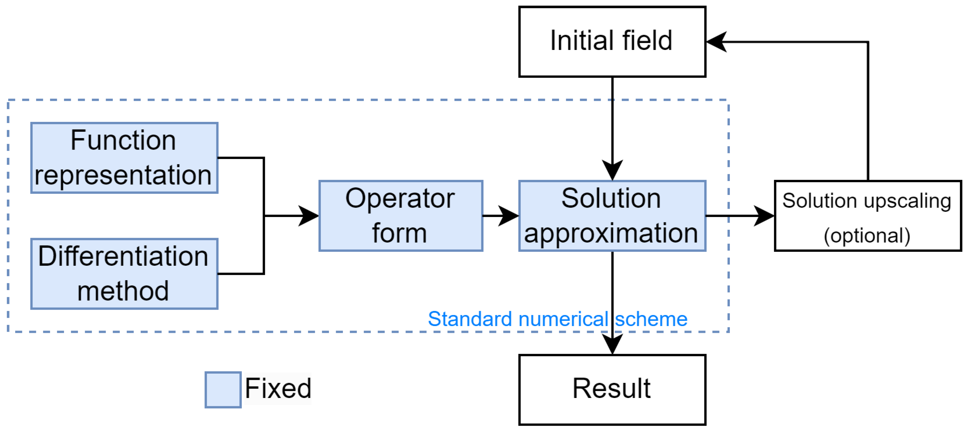
The numerical solution scheme is shown in Figure 2.
In most numerical methods, all parts are programmed so that they cannot be replaced. The fixed form of the modules allows for the creation of computationally efficient software that handles a narrow class of problems.
For example, we consider the finite-difference numerical method. For a numerical solution using a finite-difference scheme, we represent the function as the values at discrete grid points using an m × n matrix or more generally, a poly-dimensional array representation. An example of a discrete grid with dimensions m × n is shown in Equation (8).
u ¯ = u 1 , 1 u 1 , n u m , 1 u m , n
In this case, numerical differentiation is a condition that binds adjacent nodes and forms the system of linear equations. For example, we can use the first-order finite-difference scheme (the approximation order is O ( h ) , where h is the uniform grid step in discretizing the given dimension). We use forward and backward numerical differentiation for boundaries in the form of Equation (9).
u f ( x ) = u ( x + h ) u ( x ) h u b ( x ) = u ( x ) u ( x h ) h
We use the scheme described in Equation (10) for the interior points, as it is more stable.
u c ( x ) = 1 2 ( u f ( x ) + u b ( x ) ) = u ( x + h ) u ( x h ) 2 h
As the third component of the numerical PDE solution algorithm, Equations (9) and (10), together with the boundary conditions, are used to form the system of n × m equations to find the values at the grid points. Such simplicity is not typical for finite-difference schemes; usually, the expert is required to form the finite-difference schemes and solutions.
All three components are required to determine most of the numerical PDE solution algorithms. We use machine learning models to make the PDE solution more automated.
Proposed method. We choose the approximation form, determine how to take differentials with it, and optimize parameters to implement the automated solver. We briefly overview these steps in this section.
(i)
Parametric optimization. As the first component of the numerical solution, we attempt to approximate the solution u ( x , t ) of an equation L u = f with a continuous parameterized function u ¯ ( x , t ; Θ ) : R 2 R that is represented by the parameterized model. The parameter set Θ = { θ 1 , θ N } is an arbitrary set that determines the pre-defined function form. As the most straightforward example, u ( x , t ; Θ ) = θ 1 x + θ 2 t + θ 3 represents a linear regression. Moreover, it could be a neural network. In this case, the method is an extension of PINN-like models.
(ii)
Model-agnostic differentiation. As the second component, we use finite-difference schemes, such as Equations (9) and (10), and automatic differentiation as equivalent choices. We explicitly build the finite difference schemes and combine them to apply operators for higher-dimensional derivatives in order to speed up computation.
(iii)
Sobolev space optimization. To find the parameter set Θ = { θ 1 , θ N } , we use the formulation of the problem described in Equation (7) in the form (11).
min Θ | | L ¯ u ¯ ( x , t ; Θ ) f | | i + λ | | B ¯ u ¯ ( x , t ; Θ ) g | | j | X
Since the parameterized model is continuous, it is unnecessary to compute derivatives using only values at the grid points. Therefore, the main difference is that the parameter h can be arbitrarily chosen without a connection to the discretization grid X. Such solutions are usually referred to as “mesh-free”.
We note that the schemes described in Equations (9) and (10) for finite-difference analysis are proven to converge at grid points. Therefore, taking h the same as the grid resolution for these schemes is somewhat optimal. We note that we do not consider different schemes, such as x + 1 / 2 h , for brevity.
To summarize, we encode every operator to use it in the parameterized model training process. The same procedure is used for the boundary conditions. We use the optimization algorithm to obtain the optimal set of parameters Θ o p t starting from the initialization weights of the neural network Θ i n i t . The set of parameters Θ o p t minimizes the difference between the applied operator and the function approximated by the neural network function L ¯ u ¯ and the function f at all discretization points X. Furthermore, we introduce the difference between the applied boundary operator and the function g as an additional regularization.
It should be noted that such a learning process differs from the classical neural network training process, where L p norm convergence is generally considered. In this case, the convergence of the neural network is in a Sobolev space [26].
To summarize the section, we collect differences between the proposed approach and DeepXDE [27] in Table 1.
We note that DeepXDE could be expanded to the operator forms and boundary conditions shown in Table 1. However, to handle the automated solution, we must change the philosophy from a “mathematical” problem description to a less formalized one. For example, the initial and boundary conditions should be considered as one class. We should be able to define “boundary conditions” in the domain interior.
Moreover, the integration speed is also essential. Therefore, we could change Autograd to numerical differentiation, and in some cases, numerical differentiation is the only way to apply the operator to the model. We also use the “cache” technique, which is described below, to enable us to start from a reasonable initial guess.

4.3. Modular Approach

It should be noted that the proposed scheme is not unique. To address this, we propose the resulting solver module structure shown in Figure 3.
The operator encoding module includes two approaches for translating the fixed input form into the loss to optimize the model weights. The first approach considers PyTorch-based models, which could be either neural networks or simpler linear regression models. In the second approach, the model is represented as the values at the given grid point values, i.e., matrix or, in general, tensor.
The pre-processing of the two approaches differs in the differential approximation and boundary condition approximation modules. PyTorch models may be differentiated using Autograd or finite differences, whereas matrix-based models may be differentiated using only finite differences. The latter approach, in some cases, is faster since the matrix computations are used.
After that, the loss function is formed using the chosen differentiation type and optimized within the optimization module. Standard built-in PyTorch optimizers are used for this purpose.
Our experiments have shown that the problem formulation described in Equation (7) is more critical than the specific realizations of field approximations, numerical differentiation, optimization algorithms, initial field interpolation, or neural network solution upscaling. Thus, we mark the corresponding modules in the scheme as replaceable.

4.4. Caching of Approximate Models

We use initial field interpolation to achieve faster and better convergence. This is the functionality of the initial field interpolation module shown in Figure 3. The effect of the initial guess for optimization is shown in Section 5. It is performed as a “cache” of models for neural networks. As an initial step for every algorithm run, we search the library for the model of the same or another architecture with the lowest Sobolev space norm (sum over all grid points X of the functional in Equation (11)) for the given equation and boundary conditions. If the model architectures are different, we train the input architecture on values of a “cached” one.
After the algorithm is stopped, the weight of the neural network and the optimizer state (gradient value and related gradient parameters) are saved for further use.
The use of the caching technique enforces using pre-trained models as initial guesses. In some cases, the algorithm cannot leave the initial guess proximity and, thus, the algorithm incorrectly returns the initial guess as a solution without exploring the entire optimization space. The network weights are perturbed every time the best model is taken from the cache to avoid possible cases of “too good” initial guesses.
Even though the parameter’s tuning may reduce the optimization time, the overall quality of the solution remains the same across a broad range of parameter values. As a result, the proposed approach may solve ODE and PDE similarly without changing parameters. Such an approach does not challenge the classical methods. On the contrary, in the most challenging cases, the resulting solution may require correction. However, this approach allows for the comparison of two equations during the discovery process without having to stop the algorithm due to inappropriate equations for solution errors.

5. Numerical Experiments

The following experiments show the broad range of equations that could be solved with single neural network architecture and algorithm hyperparameters set. All experiments and pictures are supported by the repository (https://github.com/ITMO-NSS-team/torch_DE_solver/tree/main/examples (accessed on 7 February 2023)) with code and experimental data. The experiments show that:
  • Cache allows converging faster;
  • Adding points to the grid leads to a better solution;
  • The error between the exact and obtained solutions is negligible for equation discovery application.
We note that using neural networks does not allow for the reproduction of singularity points. Therefore, all equations are considered in the variable range where no singularities are contained. Below, the proposed approach is referred to as TEDEouS.
We used the output of Wolfram Mathematica 13’s DSolve or NDSolve as the exact solution, unless otherwise stated.
For all experiments, we attempt to search for an optimal constant parameter from the set λ { 10 4 , 10 3 , , 10 4 } to achieve the best trade-off between the speed of convergence and the quality (least possible error value) of the solution. The optimal values for the considered examples are λ = 10 3 or λ = 10 4 . In general, when the solution is unknown, the descending rate of the loss value plots can be considered as a replacement for the quality of a solution.
Several plots of the solutions to the selected problems are shown in Appendix B.

5.1. Ordinary Differential Equations

Ordinary differential equations can be used to determine possible classes of functions that could theoretically be obtained using the solution algorithm. This subsection considers two sets of equations: the Legendre equation and Painlevé transcendents.

5.1.1. Legendre Equation

The Legendre equation may determine which maximal Taylor series decomposition order may be obtained as a solution. This section considers the problem in the form of Equation (12). The solution to the problem is a Legendre polynomial of degree n.
( 1 t 2 ) u ( t ) 2 t u ( t ) + n ( n + 1 ) u = 0
Boundary conditions in the form of Equation (13) are used.
u ( 0 ) = L n ( 0 ) u ( 1 ) = d L n ( t ) d t | t = 1
In Equation (13), L n ( t ) is a Legendre polynomial of degree n. As a solution, we expect a fully restored Legendre polynomial of degree n.
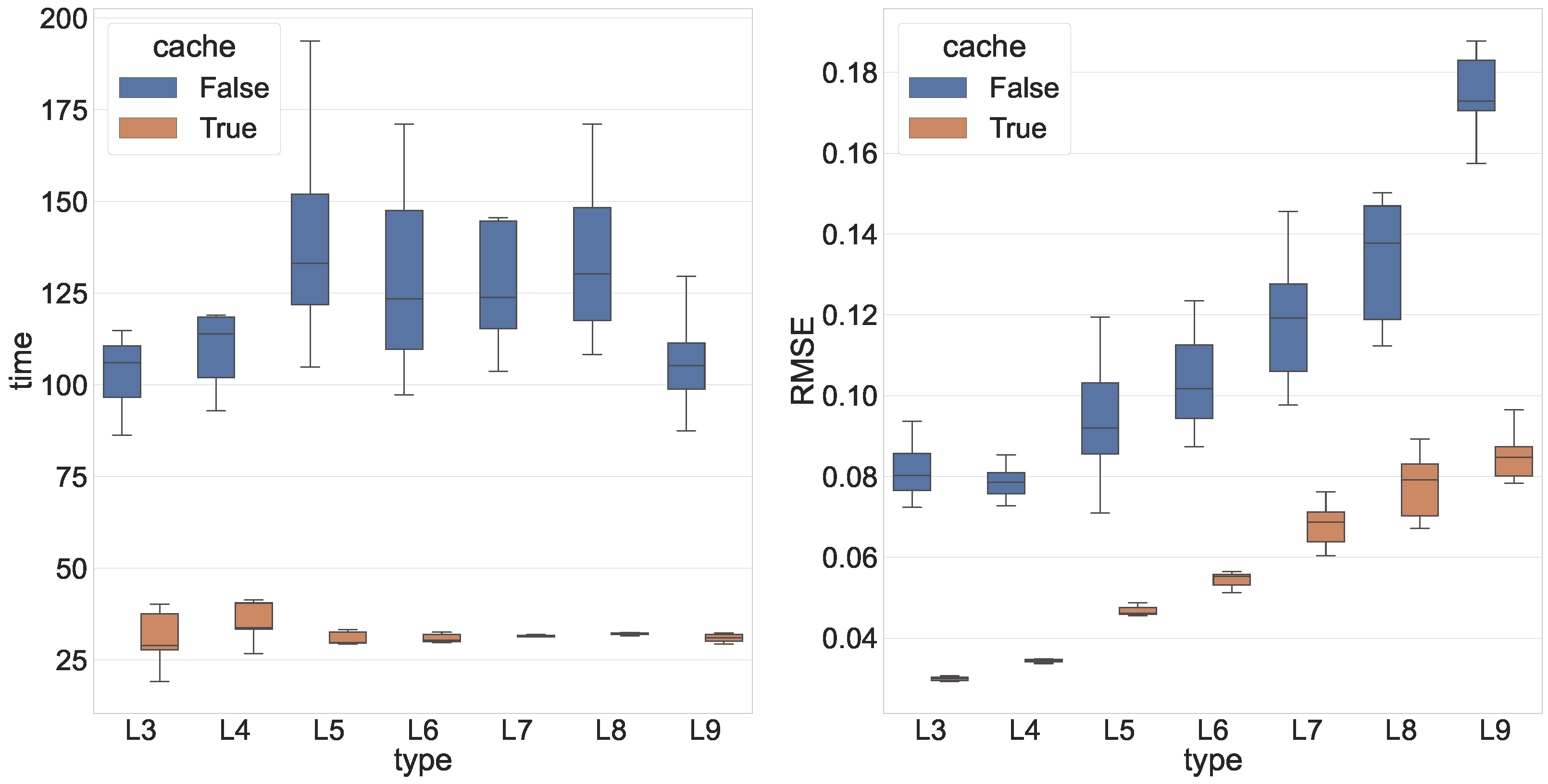
The first set of experiments involves learning the neural network parameters for n = 3 , , 9 for 100 uniformly taken points from a range t [ 0 ; 1 ] . The optimization time was recorded without (cache=false) and with the (cache=true) caching technique (see Section 4.4) for 10 runs, as shown in Figure 4 (left).
As seen in Figure 4 (left), the reasonable initial guess, as expected, makes the optimization converge faster. As a drawback, such an approach makes optimization more “rigid”. Thus, in some cases, it may become stuck in the local minima. To partially mitigate the rigidity, we perturb the initial guess parameters with a small amount of noise.
The root mean square errors (RMSEs) for the same setup are shown in Figure 4 (right). For every grid point, the error is computed using the analytical solution—Legendre polynomial values of the corresponding order in a range t [ 0 , 1 ] (the half range is taken due to the symmetry property). Since the maximal value of the Legendre polynomial on range t [ 0 , 1 ] is 1, RMSE could be interpreted as the absolute error.
In Figure 4 (right), we see that the locality of the solution described in Section 4.4 appears when the cache is used. Namely, the error spread is lower when an initial guess is used. It allows the algorithm to find the solution with a lower Sobolev space norm as a positive effect. Therefore, the initial guess allows for faster convergence, and the solution will likely have a better norm.
Overall, the ability of the solver to converge toward a Legendre polynomial solution means that the solver can converge toward any analytical solution (a solution that may be represented in the form of the Taylor series). We obtain at least the ninth term in the decomposition with good precision (less than 10% error) using 100 points, without any changes to the parameters or an increase in optimization time.
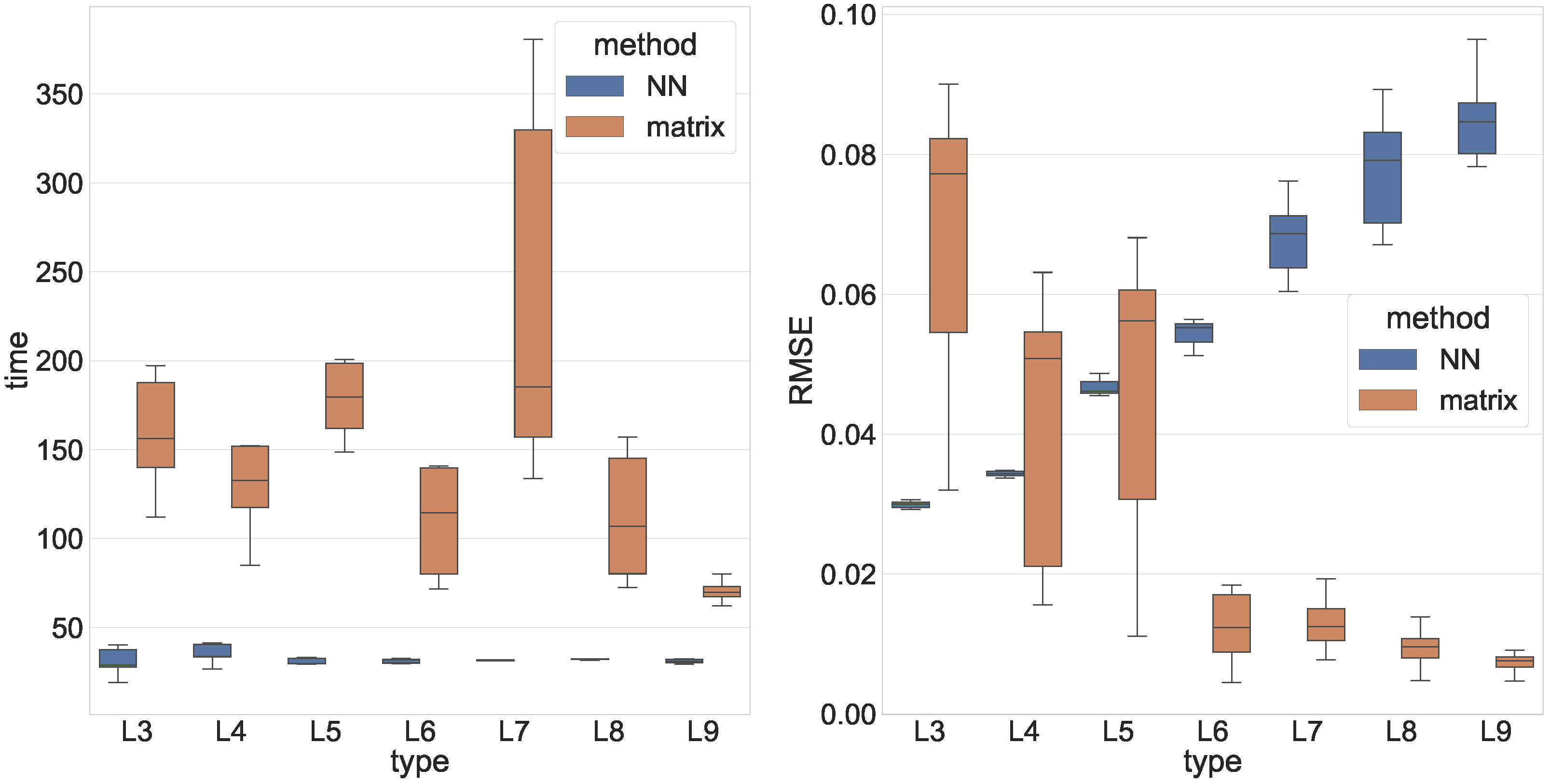
Linear model optimization. To reduce errors and show different modules, as seen in Figure 3, we utilized the matrix differentiation prototype. The results for the same grid setup for the Legendre Equation (12) are shown in Figure 5.
From the comparison of the matrix and the neural network approximation, we see that while the matrix has a lower error, it has a longer computation time. Thus, additional techniques are required, such as consequent field up-sampling or another result “caching”. However, the matrix-based algorithm is outside the scope of this paper. Therefore, further experiments were conducted using neural network approximation only.

5.1.2. Painlevé Transcendents

Painlevé transcendents are a series of differential equations. Each has a different particular function class in the solution. As the order of the transcendent increases, it becomes closer to the general hypergeometric function. In this subsection, we will consider different aspects of the Painlevé transcendent solution as an essentially non-linear ODE with variable coefficients. The scheme of functions that form the general solution of a given Painlevé transcendent is shown in Figure 6.
Exact initial and boundary-value problems are placed in Appendix A since the form of the equation is not essential for further experiments. The value range is taken, so the solution does not contain singularity points.
The Legendre equation appears as a relatively simple linear equation with variable coefficients, the Painlevé transcendents are significantly nonlinear and have a more extensive solution space than the polynomial. Additionally, the maximal sequential number of transcendent allows us to determine which class of function solver can reproduce. A hypergeometric function is the broadest possible class for a real-valued ODE solution.
We note that the solver parameters and the neural network model are the same as for the Legendre polynomial in Section 5.1.1 in most Painlevé transcendent experiments, with possibly variable stop criterion, meaning that in some cases, optimization is stopped earlier or later depending on the equation.
For the first three Painlevé transcendents, we repeat the same experimental setup as in Section 5.1.1. However, this experiment series shows convergence by changing the amount of uniformly taken points g r i d _ r e s from a value range t T . The error and optimization time distribution are shown in Figure 7. The error is computed using the Wolfram Mathematica 13 numerical solution on the points in the optimization grid.
As seen in Figure 7, a proper initial weight distribution reduces the optimization time and possibly leads to a lower error. We note that the errors are not normalized—the maximum value of the PI solution is 0.2 with a maximum error of 0.002, which is approximately 1%, and the maximum value of the PIII solution is 28.5, with a maximum error of 4, which is around 14%.
More complex transcendents have increased solving times, as shown in Figure 8 (left) (we emphasize that the logarithmic scale for time is used).
The optimization time mostly depends on the number of terms of the equation. To assess the influence of the complexity of the solution, we should use the set of equations of a similar number of terms with different solution classes, which is nearly impossible.
For all six Painlevé transcendents, the mean (for PIV–PVI, only one run was performed) error over all experiments using cache is shown in Figure 8 (right). We emphasize that the error is normalized on the maximum error achieved during all experiments for all grid points.
In summary, the algorithm error “converges” toward a solution for every transcendent without discontinuity points. Thus, the optimization problem always has a solution close to the true PDE solution in the range where the solution is analytic. However, such a statement requires more rigorous proof outside of the scope of the paper.

5.2. Partial Differential Equations

In this section, we demonstrate how the described algorithm is applied to a numerical solution to different PDE problems. We show three examples. Two canonical equations, the wave and heat equations, serve as “lower” complexity bounds. The Korteweg–de Vries equation is considered a more complex example of a non-linear equation.

5.2.1. Wave Equation

Non-physical boundary conditions. We assess the convergence of the algorithm for PDE problems. As the first example, we solve the wave equation with boundary conditions in the form of Equation (14). We understand that such conditions seem non-physical. However, as mentioned in the introduction, the main application of the method is data-driven equation discovery. We usually only have the observation field without any information about derivatives. This explains the choice of the boundary condition type for this experiment.
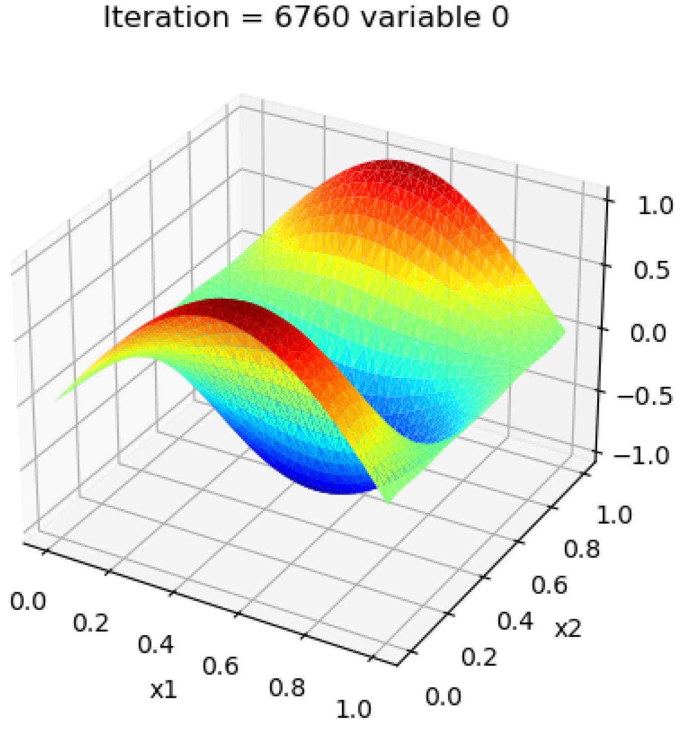
2 u ( x , t ) t 2 1 4 2 u ( x , t ) x 2 = 0 u ( 0 , t ) = u ( 1 , t ) = 0 u ( x , 0 ) = u ( x , 1 ) = sin ( π x ) ( x , t ) [ 0 , 1 ] × [ 0 , 1 ] = Ω
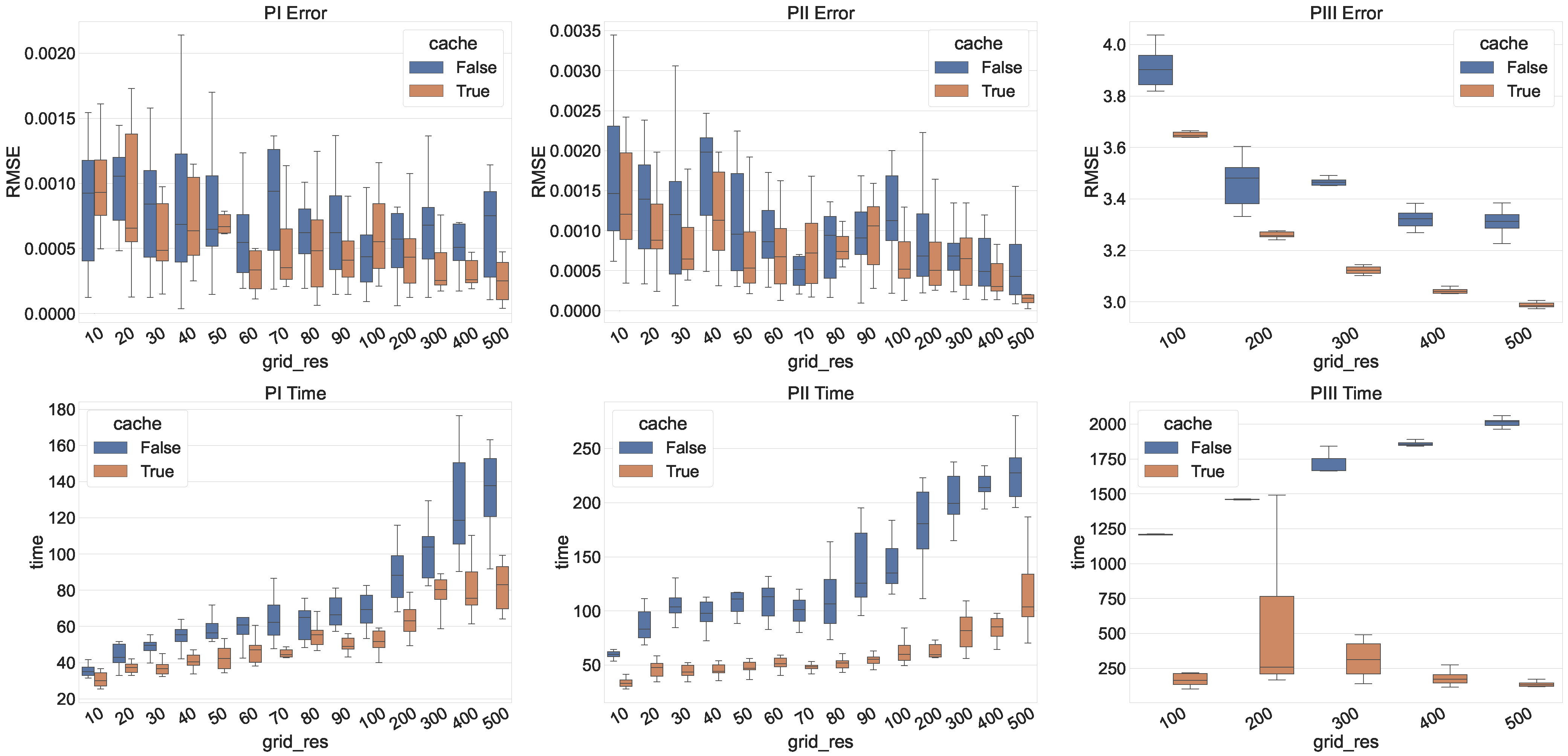
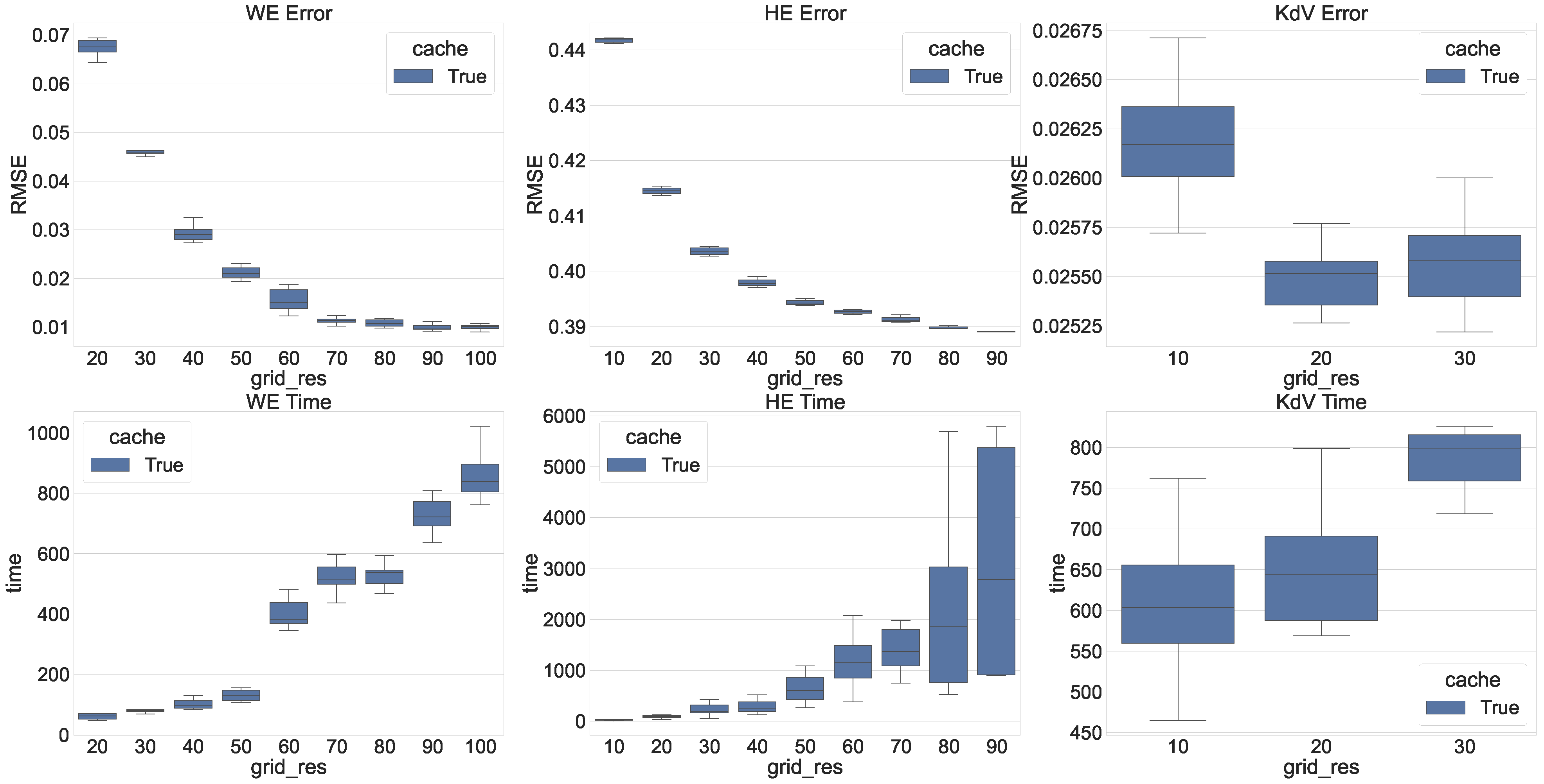
We use the formulation of Equation (6) to obtain the solution of the equation for ten runs, consequently increasing the number of points in discretization from 10 × 10 points in Ω (since the mesh is assumed uniform, it is equal to h = 1 / ( N 1 ) = 1 / 9 , where N is the number of points for time and space dimensions, i.e., we take 10 points in the range [ 0 , 1 ] including boundaries) to 100 × 100 points with the step of 100 points. As a result of the ODE experiments, we show only the “cache” version every time we start with the best possible initial weights of the neural network (see Section 4.4).
We take an analytical solution from Wolfram Mathematica 13.0 software as the exact solution. The solution has an analytical form and is taken at the grid points for each grid used in the optimization process. We record the optimization time and the root mean square error (RMSE) between the Wolfram Mathematica solution and the proposed algorithm solution on the same grid. The time and error distribution for ten runs are shown in Figure 9 (left).
Physical boundary conditions. The problem Equation (14) is equivalent to a more physically significant problem, as shown in Equation (15).
2 u ( x , t ) t 2 1 4 2 u ( x , t ) x 2 = 0 u ( 0 , t ) = u ( 1 , t ) = 0 u ( x , 0 ) = sin ( π x ) u t ( x , 0 ) = 0 ( x , t ) [ 0 , 1 ] × [ 0 , 1 ] = Ω
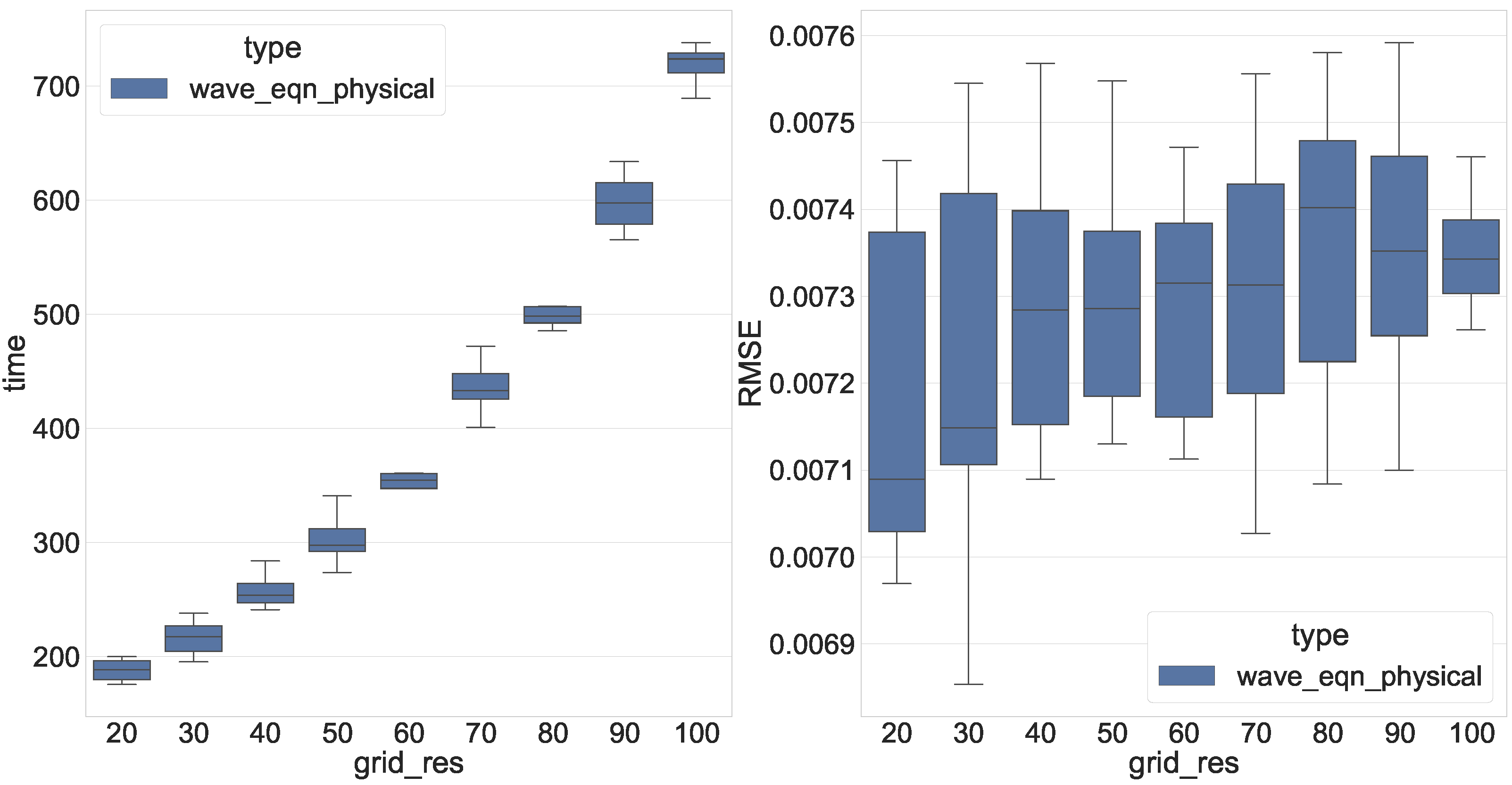
The experimental results for problem Equation (15) are shown in Figure 10.
It can be seen from Figure 10 that the error level for the problem Equation (15) is the same level as Equation (14) in Figure 9.

5.2.2. Heat Equation

The second equation is a typical parabolic type—a heat equation. To demonstrate that the algorithm can handle boundary-value problems with incompatible boundary conditions, we use the following formulation shown in Equation (16).
u ( x , t ) t 2 u ( x , t ) x 2 = 0 u ( 0 , t ) = 500 u ( x , t ) x | x = 1 = 1 u ( x , 0 ) = 0 ( x , t ) [ 0 , 1 ] × [ 0 , 1 ] = Ω
The boundary-value problem in Equation (16) for the heat equation has an analytical solution in the form of Equation (17).
u ( x , t ) = 500 + x + 8 π 2 k = 1 k = + [ exp ( 1 4 π 2 t ( 2 k 1 ) 2 ) 250 π ( 1 2 k ) + ( 1 ) k sin π x 2 ( 2 k 1 ) ( 2 k 1 ) 2 ]
We use the same grid setup for the experiments as for the wave equation in Section 5.2.1. Namely, ten runs from 10 × 10 points to 100 × 100 uniformly taken from Ω = [ 0 , 1 ] × [ 0 , 1 ] . The error is computed using the analytical solution Equation (17) with 100 first terms in the sum taken. The error and time plots are shown in Figure 9 (middle).

5.2.3. Korteweg–de Vries Equation

The Korteweg–de Vries equation (Equation (18)) was used to show a more sophisticated PDE solution.
u t + 6 u u x + u x x x = f ( x , t )
Non-physical boundary conditions. Following forcing, initial and boundary conditions were applied as shown in Equation (19). We understand that physical applications are more interested in obtaining solitary solutions [29]. However, this algorithm requires significant modifications, such as working with conditions at infinity, to obtain solitary solutions, which is part of ongoing work. In our target application—equation discovery—observation data are available only over a finite domain.
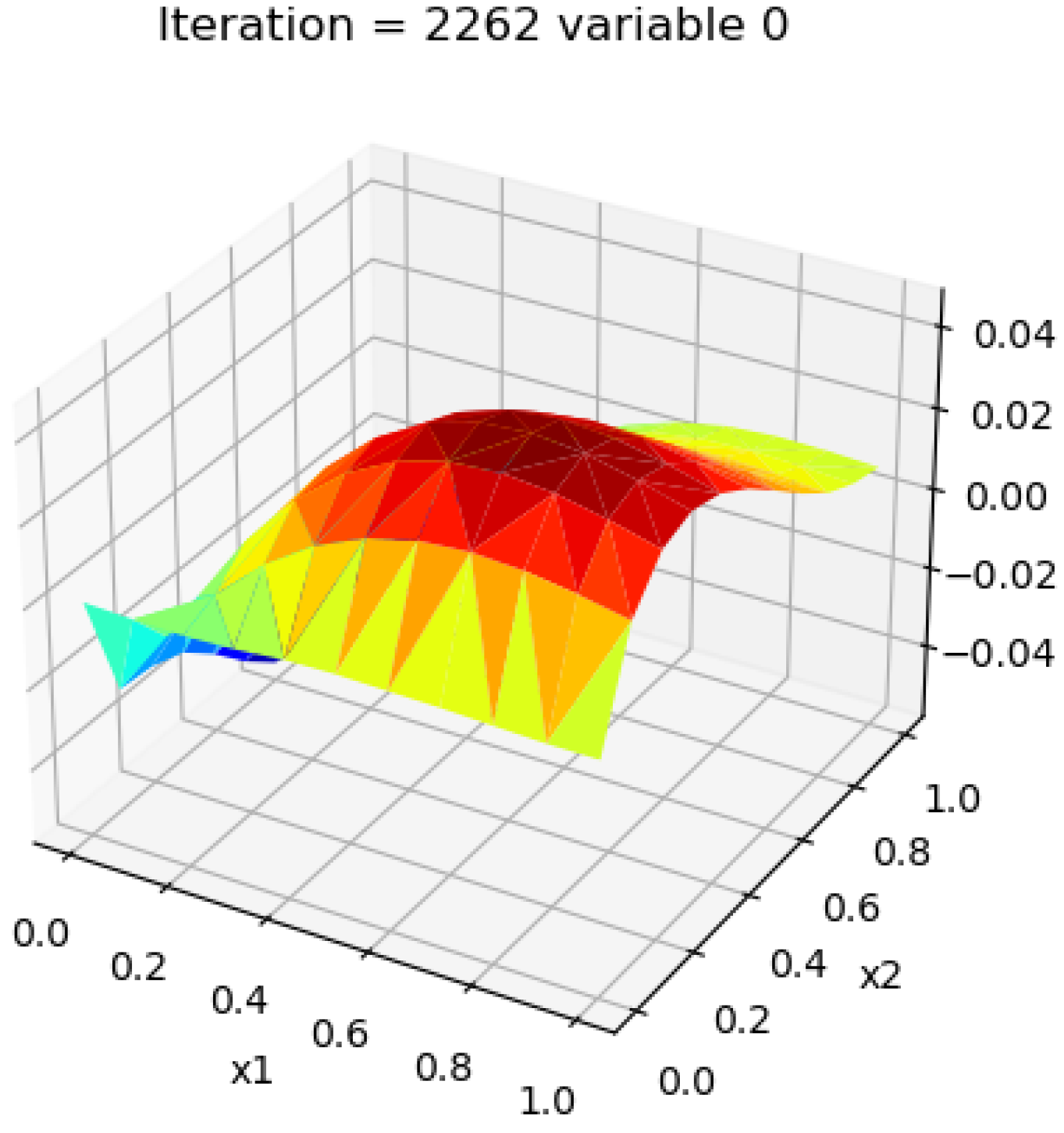
f ( x , t ) = cos t sin x u ( x , 0 ) = 0 u x x + 2 u x + u | x = 0 = 0 2 u x x + u x + 3 u | x = 1 = 0 5 u x + 5 u | x = 1 = 0 ( x , t ) [ 0 , 1 ] × [ 0 , 1 ] = Ω
Due to the extended computation time, the solution of the KdV equation was tested at the set of 10 × 10 , 20 × 20 , and 30 × 30 points uniformly taken from a range x × t [ 0 , 1 ] × [ 0 , 1 ] . The results of 10 subsequent runs for each experiment are shown in Figure 9 (right). We note that the initial solution was obtained within the 2000 s time range.
Solitary solution. Even though the algorithm in its current state cannot obtain a solitary solution directly, we perform a series of experiments that allow us to obtain the solitary solution using periodic boundary conditions. As the first step, we take the solitary solution in the form of Equation (20).
s ( x , t ) = 18 e 1 125 ( t + 25 x ) 1000 e 126 t 125 + 4 x 5 + 576 e t + x + 90 e 124 t 125 + 6 x 5 + 16 e 2 t + 9 e 2 x 5 18 e t + x 5 + 45 e t 125 + x + 40 e 126 t / 125 + 9 e 6 x / 5 2
The corresponding initial-boundary value problem has the form of Equation (21). A similar problem was solved in [30].
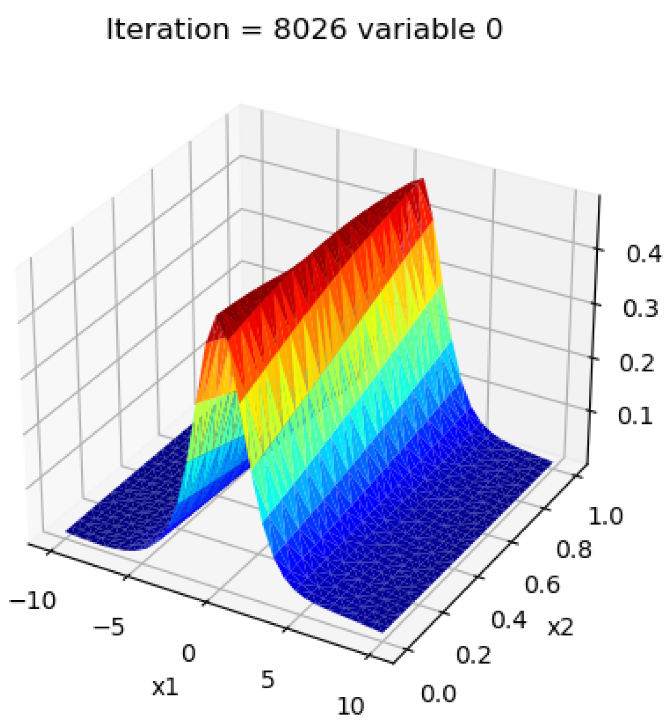
f ( x , t ) = 0 u ( x , 0 ) = s ( x , 0 ) u ( 10 , t ) = u ( 10 , t ) ( x , t ) [ 10 , 10 ] × [ 0 , 1 ] = Ω
The experimental results for the problem Equation (21) are shown in Figure 11.
Even though the computation time is higher than in the ODE case, the PDE part allows obtaining at least an approximated coarse solution, which could be used in the equation discovery algorithm within a reasonable time. Furthermore, the error is less than 10% of the maximum field value on the initial grid 10 × 10 .

6. Burgers Equation and DeepXDE Comparison

We chose a Burgers equation example to compare our approach with DeepXDE [27]. The Burgers equation boundary-value problem has the form shown in Equation (22).
u t = μ 2 u x 2 u u x u ( x , 0 ) = s i n ( π x ) u ( 1 , t ) = u ( 1 , t ) = 0 ( x , t ) [ 1 , 1 ] × [ 0 , 1 ] = Ω
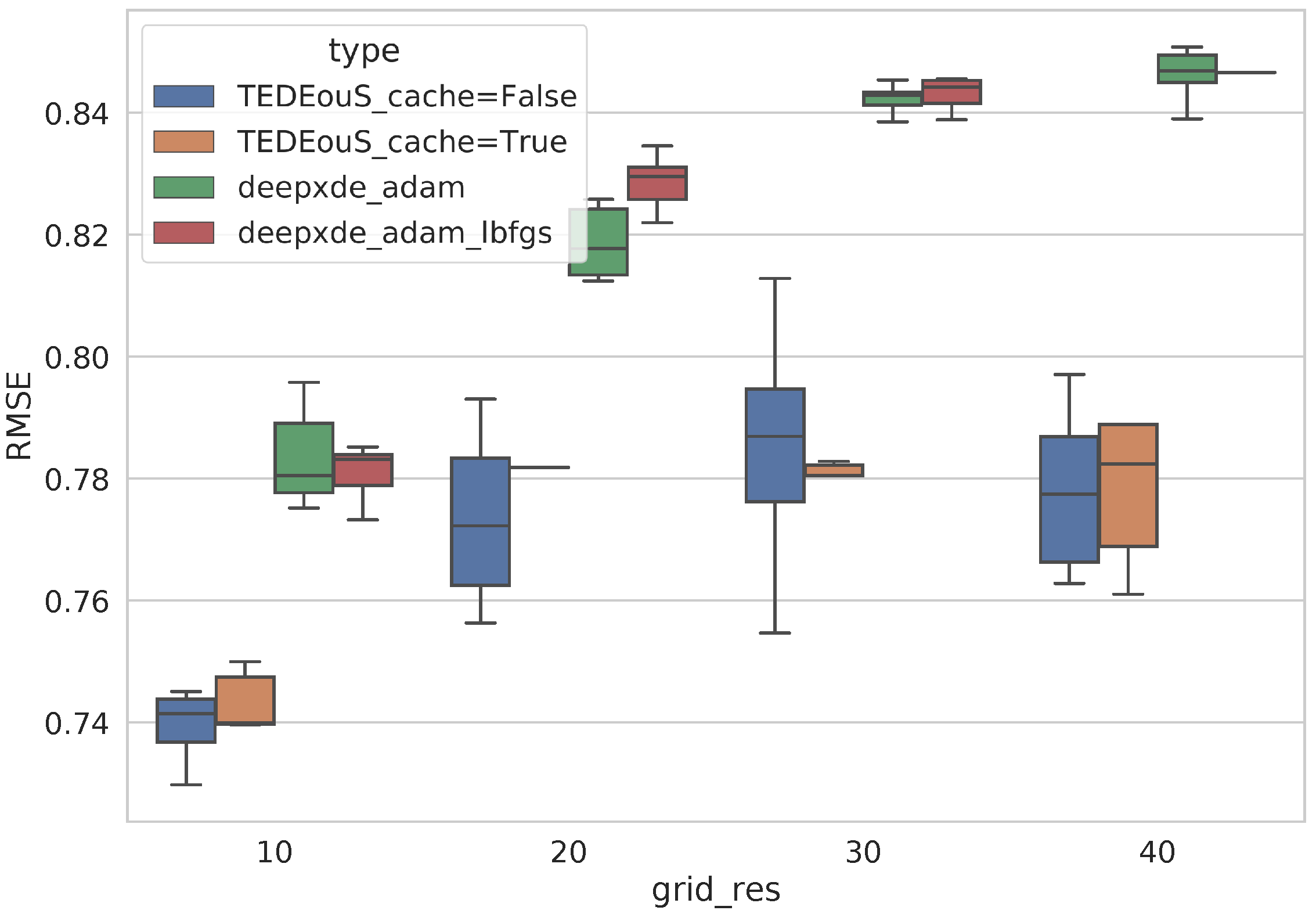
We conducted two experiments for each tool to show the best cases for the two tools. The first series of experiments shows how both tools work with the default architecture proposed in the DeepXDE example. The second series was conducted to show the good sides of both tools. For the described approach, we enable the cache to reduce optimization time. For DeepXDE, we add additional LBFGS training after the Adam one. The RMSE error computed with respect to the analytical example provided in the DeepXDE example is shown in Figure 12.
The optimization results obtained using the two tools cannot be directly compared because the described approach uses the PyTorch library for working with neural networks while DeepXDE uses TensorFlow, so it may be considered a neural network optimization difference between backends. Therefore, we do not claim that the described approach provides a better solution.
The optimization times for two different experiments are shown in Figure 13.
In this case, we do not claim that the described approach is faster than DeepXDE. However, the cache drastically reduces the integration time, whereas additional LBFGS optimization in DeepXDE significantly increases it. Moreover, one point toward the described approach speed is that DeepXDE uses the “lazy computation” mode for TensorFlow, meaning that the computation graph is precompiled and, thus, optimizes faster.

7. Conclusions

The paper proposes a unified numerical differential equation solver based on optimization methods. It has the following advantages:
  • It can solve ODE and PDE without the involvement of an expert after the algorithm launch, which is most useful for data-driven equation discovery methods;
  • It has good precision for equation solution applications and has tools to trade the precision with integration time in both directions;
  • It has a flexible modular structure. The modules could be replaced to achieve better speed or better precision.
The differences from the existing solutions are:
  • More machine learning approaches to differential equation initial-boundary value problems that allow solving non-canonical boundary-value problems, and a wider class of problems to move toward better equation discovery using automated solutions;
  • Reduced optimization times;
  • Possibility to use different parameterized models.
We note that the universal approximation theorem does not work for Sobolev spaces directly. Therefore, for some equations, one may experience incorrect solutions, as shown in [31], or do not achieve convergence at all. The convergence study in Sobolev spaces is also part of ongoing work. During the experimental studies, we found the following disadvantages:
  • Extended optimization time, which in some cases makes the discovery process non-viable;
  • To work with physical problems, it is necessary to be able to work with models that allow reproducing special functions, including non-differentiable ones;
  • To work with physical problems, the extension of boundary condition types is required.
We propose several directions for speeding up the optimization process:
  • Use of the power of GPU to perform optimization using fast memory and built-in matrix instructions;
  • Better usage of initial approximation;
  • Usage of the “lazy computation” mode, i.e., the precompiled computational graph.
As part of other possible research directions, we highlight the following:
  • The optimization problem statement using weak formulation to expand the possible class of solved equations;
  • System solutions in strong and weak forms;
  • Expand work with neural networks using Fourier layers [32] and adaptive regularization [33].
We emphasize, once again, all solutions were obtained without significant algorithm parameter changes, which is the philosophy of the automated solver that could be used in equation discovery methods.

Funding

This research is financially supported by The Russian Scientific Foundation, Agreement no. 21-71-00128.

Data Availability Statement

All experimental data and scripts that allow reproducing experiments are available at the GitHub repository https://github.com/ITMO-NSS-team/torch_DE_solver, accessed on 7 February 2023.

Conflicts of Interest

The authors declare no conflict of interest. The funders had no role in the design of the study; in the collection, analyses, or interpretation of data; in the writing of the manuscript; or in the decision to publish the results.

Appendix A. Painlevé Boundary-Value Problems

For all equations α = β = γ = δ = 1 .
Painlevé I:
u ( t ) = 6 u ( t ) 2 + t u ( 0 ) = 0 u ( 0 ) = 0 t [ 0 ; 1 ]
Painlevé II:
u ( t ) = α + 2 u ( t ) 3 + t u ( t ) u ( 0 ) = 0 u ( 0 ) = 0 t [ 0 ; 1 ]
Painlevé III:
t u ( t ) u ( t ) = δ t u ( t ) u ( t ) + t u ( t ) 2 + α u ( t ) 3 + + β u ( t ) + γ t u ( t ) 4 u ( 1 ) = 0 u ( 1 ) = 0 t [ 0.25 ; 2.1 ]
Painlevé IV:
u ( t ) u ( t ) = β + 2 t 2 α u ( t ) 2 + + 1 2 u ( t ) 2 + 3 u ( t ) 4 2 + 4 t u ( t ) 3 u ( 1 ) = 0 u ( 1 ) = 0 t [ 1 / 4 ; 7 / 4 ]
Painlevé V:
2 t 2 ( 1 u ( t ) ) u ( t ) u ( t ) = 2 β + + 2 u ( t ) 2 α + 3 β δ t 2 + γ t + t u ( t ) u ( t ) 6 β + 3 t 2 u ( t ) 2 + 2 t u ( t ) + + t 2 u ( t ) 2 2 u ( t ) 3 ( 3 α + β + t ( γ + δ t ) ) 2 α u ( t ) 5 + 6 α u ( t ) 4 u ( 0.9 ) = 3 u ( 1.2 ) = 4 t [ 0.9 ; 1.2 ]
Painlevé VI:
c 6 , 0 + c 6 , 1 u ( t ) + c 6 , 2 u ( t ) 2 + c 6 , 3 u ( t ) 3 + c 6 , 4 u ( t ) 4 + + c 6 , 5 u ( t ) 5 α u ( t ) 6 + c 6 , 6 u ( t ) u ( t ) + c 6 , 7 u ( t ) 2 u ( t ) + + c 6 , 8 u ( t ) 3 u ( t ) + + c 6 , 9 u ( t ) 2 + c 6 , 10 u ( t ) u ( t ) 2 + + c 6 , 11 u ( t ) 2 u ( t ) 2 + c 6 , 12 u ( t ) u ( t ) + c 6 , 13 u ( t ) 2 u ( t ) + + c 6 , 14 u ( t ) 3 u ( t ) = 0 c 6 , 0 = t 3 β c 6 , 1 = 2 β t 2 ( t + 1 ) c 6 , 2 = t ( β δ + t ( α + δ + β ( t + 4 ) + γ ( t 1 ) ) ) c 6 , 3 = 2 t ( α ( t + 1 ) + β ( t + 1 ) + ( t 1 ) ( γ + δ ) ) c 6 , 4 = α + γ α t ( t + 4 ) t ( β + γ + δ ( t 1 ) ) c 6 , 5 = 2 α ( t + 1 ) c 6 , 6 = ( t 1 ) t 3 c 6 , 7 = t t t 2 + t 3 + 1 c 6 , 8 = ( t 1 ) t ( 2 t 1 ) c 6 , 9 = 1 2 ( t 1 ) 2 t 3 c 6 , 10 = ( t 1 ) 2 t 2 ( t + 1 ) c 6 , 10 = 3 2 ( t 1 ) 2 t 2 c 6 , 11 = ( t 1 ) 2 t 3 c 6 , 12 = ( t 1 ) 2 t 2 ( t + 1 ) c 6 , 13 = ( t 1 ) 2 t 2 u ( 1.2 ) = u ( 1.4 ) = 2 t [ 1.2 ; 1.4 ]

Appendix B. Solution Plots

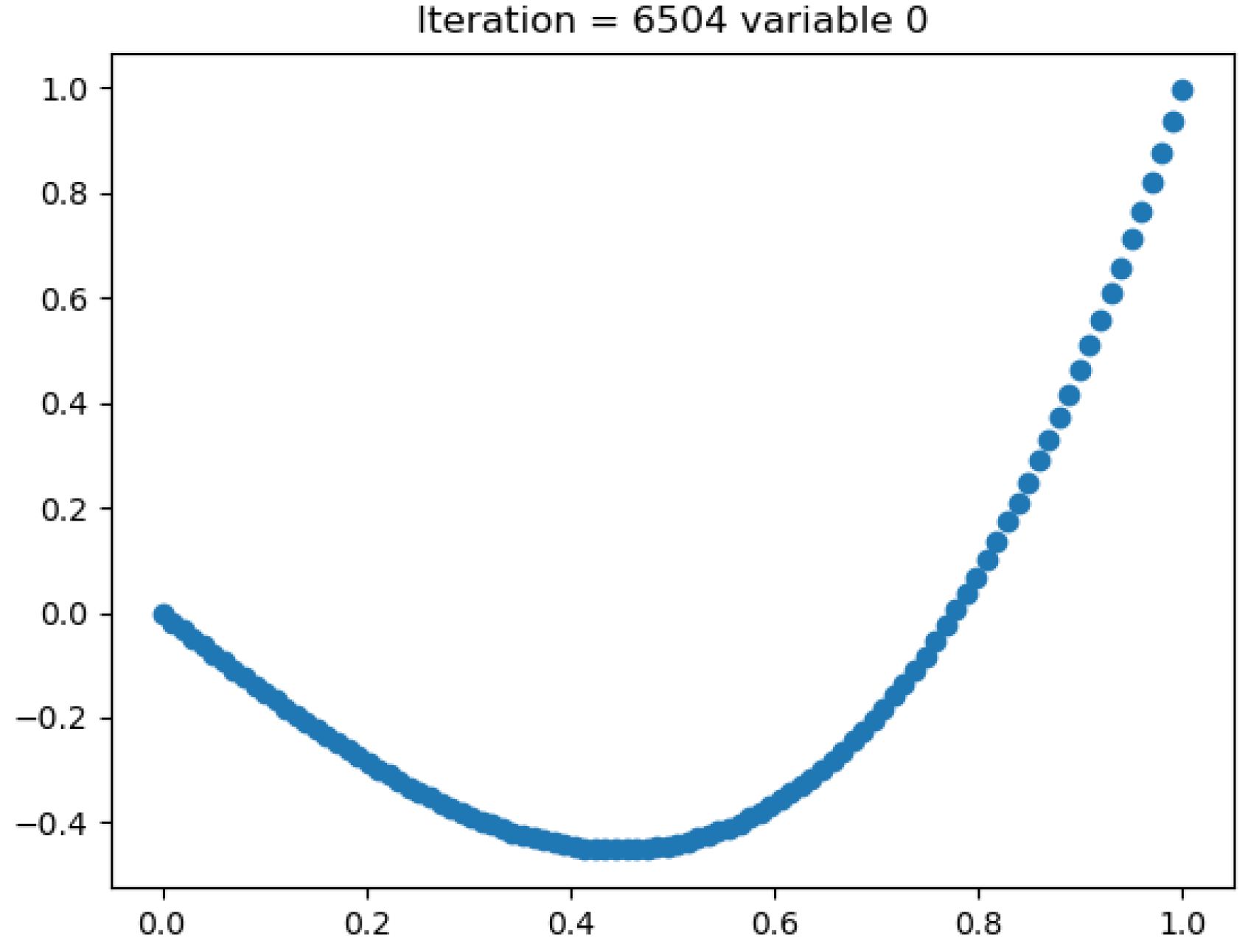
Figure A1. Solution to Legendre Equation (12), n = 2 .
Mathematics 11 01787 g0a1
Figure A2. Solution to Painlevé PIII transcendent Equation (A3).
Mathematics 11 01787 g0a2
Figure A3. Solution to wave Equation (14).
Mathematics 11 01787 g0a3
Figure A4. Solution to the non-physical initial-boundary value problem of the KdV equation, as described by Equation (19).
Mathematics 11 01787 g0a4
Figure A5. Solution to the non-physical initial-boundary value problem of the KdV equation, as described by Equation (21).
Mathematics 11 01787 g0a5

References

  1. Rao, R.; Lin, Z.; Ai, X.; Wu, J. Synchronization of epidemic systems with Neumann boundary value under delayed impulse. Mathematics 2022, 10, 2064. [Google Scholar] [CrossRef]
  2. Zhao, Y.; Wang, L. Practical Exponential Stability of Impulsive Stochastic Food Chain System with Time-Varying Delays. Mathematics 2023, 11, 147. [Google Scholar] [CrossRef]
  3. Maslyaev, M.; Hvatov, A.; Kalyuzhnaya, A.V. Partial differential equations discovery with EPDE framework: application for real and synthetic data. J. Comput. Sci. 2021, 53, 101345. [Google Scholar] [CrossRef]
  4. Rudy, S.H.; Brunton, S.L.; Proctor, J.L.; Kutz, J.N. Data-driven discovery of partial differential equations. Sci. Adv. 2017, 3, e1602614. [Google Scholar] [CrossRef] [Green Version]
  5. Long, Z.; Lu, Y.; Dong, B. PDE-Net 2.0: Learning PDEs from data with a numeric-symbolic hybrid deep network. J. Comput. Phys. 2019, 399, 108925. [Google Scholar] [CrossRef] [Green Version]
  6. Rackauckas, C.; Nie, Q. Confederated modular differential equation APIs for accelerated algorithm development and benchmarking. Adv. Eng. Softw. 2019, 132, 1–6. [Google Scholar] [CrossRef] [Green Version]
  7. Hindmarsh, A.C.; Brown, P.N.; Grant, K.E.; Lee, S.L.; Serban, R.; Shumaker, D.E.; Woodward, C.S. SUNDIALS: Suite of nonlinear and differential/algebraic equation solvers. ACM Trans. Math. Softw. (TOMS) 2005, 31, 363–396. [Google Scholar] [CrossRef]
  8. Morton, K.W.; Mayers, D.F. Numerical Solution of Partial Differential Equations: An Introduction; Cambridge University Press: Cambridge, UK, 2005. [Google Scholar]
  9. Thomas, J.W. Numerical Partial Differential Equations: Finite Difference Methods; Springer Science & Business Media: Berlin/Heidelberg, Germany, 2013; Volume 22. [Google Scholar]
  10. Ŝolín, P. Partial Differential Equations and the Finite Element Method; John Wiley & Sons: Hoboken, NJ, USA, 2005. [Google Scholar]
  11. Pavlovic, A.; Fragassa, C. Geometry optimization by fem simulation of the automatic changing gear. Rep. Mech. Eng. 2020, 1, 199–205. [Google Scholar] [CrossRef]
  12. Scroggs, M.W.; Baratta, I.A.; Richardson, C.N.; Wells, G.N. Basix: A runtime finite element basis evaluation library. J. Open Source Softw. 2022, 7, 3982. [Google Scholar] [CrossRef]
  13. Burns, K.J.; Vasil, G.M.; Oishi, J.S.; Lecoanet, D.; Brown, B.P. Dedalus: A flexible framework for numerical simulations with spectral methods. Phys. Rev. Res. 2020, 2, 023068. [Google Scholar] [CrossRef] [Green Version]
  14. Li, Z.; Kovachki, N.; Azizzadenesheli, K.; Liu, B.; Bhattacharya, K.; Stuart, A.; Anandkumar, A. Neural operator: Graph kernel network for partial differential equations. arXiv 2020, arXiv:2003.03485. [Google Scholar]
  15. Li, Z.; Kovachki, N.; Azizzadenesheli, K.; Liu, B.; Bhattacharya, K.; Stuart, A.; Anandkumar, A. Fourier neural operator for parametric partial differential equations. arXiv 2020, arXiv:2010.08895. [Google Scholar]
  16. Zwillinger, D.; Dobrushkin, V. Handbook of Differential Equations; CRC Press: Boca Raton, FL, USA, 2021. [Google Scholar]
  17. Rackauckas, C.; Ma, Y.; Martensen, J.; Warner, C.; Zubov, K.; Supekar, R.; Skinner, D.; Ramadhan, A. Universal Differential Equations for Scientific Machine Learning. arXiv 2020, arXiv:2001.04385. [Google Scholar]
  18. Hindmarsh, A.C. ODEPACK, a systematized collection of ODE solvers. In Scientific Computing; Lawrence Livermore National Laboratory: Livermore, CA, USA, 1983; pp. 55–64. [Google Scholar]
  19. Hindmarsh, A.C. ODEPACK: Ordinary Differential Equation Solver Library; Astrophysics Source Code Library: Record ascl:1905.021. May 2019. Available online: https://ui.adsabs.harvard.edu/abs/2019ascl.soft05021H (accessed on 7 February 2023).
  20. Ahnert, K.; Mulansky, M. Odeint–solving ordinary differential equations in C++. AIP Conf. Proc. 2011, 1389, 1586–1589. [Google Scholar]
  21. Rackauckas, C.; Innes, M.; Ma, Y.; Bettencourt, J.; White, L.; Dixit, V. Diffeqflux.jl-A julia library for neural differential equations. arXiv 2019, arXiv:1902.02376. [Google Scholar]
  22. Liu, S.; Wang, T.; Zhang, Y. A Functional Package for Automatic Solution of Ordinary Differential Equations with Spectral Methods. arXiv 2016, arXiv:1608.04815. [Google Scholar]
  23. Raissi, M.; Perdikaris, P.; Karniadakis, G.E. Physics-informed neural networks: A deep learning framework for solving forward and inverse problems involving nonlinear partial differential equations. J. Comput. Phys. 2019, 378, 686–707. [Google Scholar] [CrossRef]
  24. Lu, L.; Jin, P.; Karniadakis, G.E. Deeponet: Learning nonlinear operators for identifying differential equations based on the universal approximation theorem of operators. arXiv 2019, arXiv:1910.03193. [Google Scholar]
  25. Sirignano, J.; Spiliopoulos, K. DGM: A deep learning algorithm for solving partial differential equations. J. Comput. Phys. 2018, 375, 1339–1364. [Google Scholar] [CrossRef] [Green Version]
  26. Czarnecki, W.M.; Osindero, S.; Jaderberg, M.; Swirszcz, G.; Pascanu, R. Sobolev Training for Neural Networks. In Proceedings of the NIPS, Long Beach, CA, USA, 4–9 December 2017. [Google Scholar]
  27. Lu, L.; Meng, X.; Mao, Z.; Karniadakis, G.E. DeepXDE: A deep learning library for solving differential equations. SIAM Rev. 2021, 63, 208–228. [Google Scholar] [CrossRef]
  28. Maslyaev, M.; Hvatov, A. Solver-Based Fitness Function for the Data-Driven Evolutionary Discovery of Partial Differential Equations. In Proceedings of the 2022 IEEE Congress on Evolutionary Computation (CEC), Padua, Italy, 18–23 July 2022; pp. 1–8. [Google Scholar]
  29. Nguyen, L.T.K. Modified homogeneous balance method: Applications and new solutions. Chaos Solitons Fractals 2015, 73, 148–155. [Google Scholar] [CrossRef]
  30. Arnold, D.N.; Winther, R. A superconvergent finite element method for the Korteweg-de Vries equation. Math. Comput. 1982, 38, 23–36. [Google Scholar] [CrossRef] [Green Version]
  31. Göküzüm, F.S.; Nguyen, L.T.K.; Keip, M.A. An artificial neural network based solution scheme for periodic computational homogenization of electrostatic problems. Math. Comput. Appl. 2019, 24, 40. [Google Scholar] [CrossRef] [Green Version]
  32. Wang, S.; Wang, H.; Perdikaris, P. On the eigenvector bias of Fourier feature networks: From regression to solving multi-scale PDEs with physics-informed neural networks. Comput. Methods Appl. Mech. Eng. 2021, 384, 113938. [Google Scholar] [CrossRef]
  33. Wang, S.; Yu, X.; Perdikaris, P. When and why PINNs fail to train: A neural tangent kernel perspective. J. Comput. Phys. 2022, 449, 110768. [Google Scholar] [CrossRef]
Figure 1. Rough classification of differential equation solvers. A classification that correspondingly may be applied to the equation is shown with ODE (violet), PDE (grey), or both.
Mathematics 11 01787 g001
Figure 2. General numerical method for solving differential equations using numerical schemes.
Mathematics 11 01787 g002
Figure 3. Module structure of the solver scheme (the green parts are replaceable).
Mathematics 11 01787 g003
Figure 4. Legendre polynomial solution time in seconds (left) and solution error (right). The type is the order of polynomial n in Equation (12); different colors (cache = false) and (cache = true) cases are shown.
Mathematics 11 01787 g004
Figure 5. Legendre polynomial solution time (left) and solution error (right). The order of the polynomial n in Equation (12) is indicated by the type of curve, while different colors represent different approximations, i.e., neural network-based and matrix-based.
Mathematics 11 01787 g005
Figure 6. Scheme of the solution of the Painlevé transcendent “complexity”. Each class of functions contains the previous one. The color coding indicates the predicted relative “performance” of a conventional solver for each transcendent.
Mathematics 11 01787 g006
Figure 7. A summary of Painlevé I–III experiment runs. Different colors represent runs with and without an initial guess.
Mathematics 11 01787 g007
Figure 8. Mean time (in seconds) in the logarithmic scale of the optimization for each Painlevé transcendent (left) and mean error ratio (right) (1.0 is the maximal error for each equation); the maximal error for PI–PII is at the 10 grid point, which is not shown.
Mathematics 11 01787 g008
Figure 9. Summary of all PDE experiments: upper row errors and lower time. From (left) to (right)—wave equation, heat equation, and Korteweg–de Vries equation.
Mathematics 11 01787 g009
Figure 10. Results of the numerical solution to problem Equation (15) for a different number of discretization points. Computation time (left) and RMSE (right). All experiments were performed with cache=True.
Mathematics 11 01787 g010
Figure 11. Results of the numerical solution to problem Equation (11) for a different number of discretization points. Computation time (left) and RMSE with respect to the analytical solution Equation (20) (right). All experiments were performed with cache=True.
Mathematics 11 01787 g011
Figure 12. RMSE with respect to the analytical solution: orange—proposed approach without cache, blue—with cache, green—DeepXDE without additional LBFGS refinement, red—with LBFGS refinement.
Mathematics 11 01787 g012
Figure 13. Optimization times for different methods: orange—proposed approach without cache, blue—with cache, green—DeepXDE without additional LBFGS refinement, red—with LBFGS refinement.
Mathematics 11 01787 g013
Table 1. Comparison of the proposed approach with DeepXDE for some parameters.
ModuleDeepXDEProposed Approach
ApproximatorNN (TensorFlow—dense,
Fourier kernel layers)
Parameterized model
(PyTorch)
DifferentiationAutogradAutograd,
numerical differentiation
Operator formConstant coefficients,
variable coefficients (no examples)
Time- and spatial-
variable coefficients
BC formDirichlet, Neumann, Robin,
IC, GeneralBC (no examples)
Arbitrary
Disclaimer/Publisher’s Note: The statements, opinions and data contained in all publications are solely those of the individual author(s) and contributor(s) and not of MDPI and/or the editor(s). MDPI and/or the editor(s) disclaim responsibility for any injury to people or property resulting from any ideas, methods, instructions or products referred to in the content.