A Study of Assessment of Casinos’ Risk of Ruin in Casino Games with Poisson Distribution

Abstract

Gambling, as an uncertain business involving risks confronting casinos, is commonly analysed using the risk of ruin (ROR) formula. However, due to its brevity, the ROR does not provide any implication of nuances in terms of the distribution of wins/losses, thus causing the potential failure of unravelling exceptional and extreme cases. This paper discusses the mathematical model of ROR using Poisson distribution theory with the consideration of house advantage (a) and the law of large numbers in order to compensate for the insufficiency mentioned above. In this discussion, we explore the relationship between cash flow and max bet limits in the model and examine how these factors interact in influencing the risk of casino bankruptcy. In their business nature, casinos operate gambling businesses and capitalize on the house advantage favouring them. The house advantage of the games signifies casinos’ profitability, and in addition, the uncertainty inevitably poses a certain risk of bankruptcy to them even though the house advantage favours them. In this paper, the house advantage is incorporated into our model for a few popular casino games. Furthermore, a set of full-range scales is defined to facilitate effective judgment on the levels of risk confronted by casinos in certain settings. Some wagers of popular casino games are also exemplified with our proposed model.

1. Introduction

Like other businesses, casinos always watch out for both profitability and risks and try to strike the right balance between the two. Their profitability is simply determined by the house advantage and max bet limit (bet size). The max bet limit is one of the policies established by a casino and the jurisdiction that governs the casino mainly for protecting its gambling business. The higher the house advantages and max bet limits, the higher the casino’s profits. However, the downside of higher limits is that they pose higher threats of bankruptcy to casinos. In fact, there is a kind of gambler called a “high roller” who can afford to make a high-stake bet as high as tens of thousands of US dollars. Some of these “whales” (the nickname for the highest-spending kind of high roller) can even bet a hundred thousand dollars a hand, and usually they bet a limited number of hands against the casinos. Therefore, they can possibly make a small casino bankrupt [1]. To lessen the risk, casinos need to sacrifice the high profit with respect to their bankroll and max bet limits. What can casinos do in order to lower the risk of a game?

There are a number of popular gambling games offered in casinos, such as baccarat, roulette, blackjack, Sic Bo and craps. The games are fundamentally categorized into skilled games and non-skilled games [2,3]. Skilled games require gamblers to decide on how they play during gameplay, which somewhat influences their payout rates (also namely house advantages) to a certain extent, whereas non-skilled games are those that do not require gamblers to make any decisions except for the wagering amounts, and the payout rates are fixed. Among those, baccarat, roulette, Sic Bo and craps are non-skilled games, which are chosen for use in the entire paper for avoiding the uncertainty caused by human behaviours in skilled games. The house advantage (a) is a percentage that reflects not just the probability of winning, but also the amount of casino win for a particular wager of a game in the long-run. Therefore, house advantages represent the profit rates of casino games. A game has one or more distinct wagers, i.e., ways to bet. Taking baccarat as an example, there are at least four wagers, including banker, player, tie, etc. Each wager has a probabilistic model, determining the probability that a certain event will occur [4]. To calculate the house advantage of a wager of a game, we have to provide the probability of occurrence of a certain event and the amount that the casinos will pay for a winning stake (or the payoff rate). For calculating the house advantage, it often relates to the expected value ($\mu$) and $\mu$ can be adopted to calculate how much money a player can expect to win/lose in the long-run on a particular wager. As shown in the following formula, $\mu$ is the algebraic sum of a series of net payouts and probabilities of all possible alternatives:

$$\mu =\sum \left(P\left(X_i\right)\times X_i\right)$$

(1)

Here, $X_i$ denotes the gambling event and $P\left(X_i\right)$ denotes the probability of $X_i$. Simply speaking, $\mu$ is an average value of a random variable in the long-run. It is a mathematical tool widely used in financial and gambling estimations for dealing with uncertain events. In a gambling business, the negative of the expected value is commonly expected since the favour is normally on the casino’s side, and the house advantage is calculated simply by $a=-\mu \times 100\%$, whereas $\mu$ is used to deal with the evaluation of the worthiness of probabilistic choices in this case. However, for the risk assessment, the house advantage surely helps alleviate the risk of bankruptcy, but we have no clue to what extent the risk can be lowered. The number of trials also dictates the risk of the casino business. According to the law of large numbers (a.k.a. the 1st Law of Probability), if a large number of trials take place for a random event, the average of the trial outcomes should be close to the expected value or theoretical outcomes. This is an important underlying theorem of probability. With a sufficiently large sample, there will be a very high probability that the average of the trials will approach the expected value, thus making the casino earn the profit as expected. Theoretically, the more trials there are, the lower the risk will be. The number of trials is in turn the result closely related to the casino’s bankroll and the max bet limit allowed. Explicitly, the number of trials (n) is the division of the bankroll by max bet limit.

With the brief discussion of the ideas, the listed items below are the contributions we are going to present in this work:

• We establish a formal basis for the risk of ruin through deriving the Poisson process, which contains the following factors: the win probability (p), the house advantage (a) and the predicted maximum number of bets (n).
• In addition, we provide a proof of the properties of the proposed formula, which satisfies monotonicity and also contains probabilistic features. This formula is used to illustrate the relevant cases in real casinos by setting changes of the factors in our proposed model.
• We explore and derive the experimental results of various models, and devise a novel measurement method with the risk of ruin scale, which aims at normalizing the risk levels and concretely reflecting the current risk statuses.

The paper is organized as follows. Section 2 discusses the related work on the probability of bankruptcy risk by various means and models. Section 3 presents the derivation and proof of the proposed model under the Poisson process. Section 4 simulates and discusses various ROR models for performance evaluation. Section 5 introduces a novel Risk of Ruin Scale measurement standard for risk assessment. Finally, we conclude the paper in Section 6.

2. Literature Review

As betting between gamblers and casinos works under probabilities, the risk of ruin always decreases in the long-term when casinos have a favourable house advantage and overall positive expectancy. For the risk of ruin (ROR) calculation, the higher the max betting, the higher the probability of bankruptcy of casinos with a given size of bankroll (or capital base). Further, the risk decreases as the number of bets increases and the casino has a larger bankroll than the gambler [5]. The ROR prediction model given in [6,7] is the probability of losing the entire startup bankroll before achieving the profitability goal. In [8], the author introduces an analogy to the ruin formula $\mathit{Pro}\left(n\right)=\frac{1}{1+{\left(1+a\right)}^n}$, which outlines the probability of a gambler being able to catch up to the casino bankroll that decreases exponentially in the number of steps n, if the casino has the house advantage (a) in each betting. This provides a general means to estimate the conception of guaranteeing sustainability with a given number of plays, but the formula does not take account of the win probability (p) of a casino in a game [9]. It is well understood that gambling is challenging when success depends on obtaining certain benefits relative to the odds [10]. Therefore, one of the advanced models [11], which has been introduced to describe the behaviour of gamblers and the strategy of casinos with respect to time, is the discrete-time-based risk model [12]. Simply speaking, it describes the casino bankroll’s level only in discrete time moments. Although this model is not very applicable in practice, it has been extensively investigated by many studies in theoretical results [13]. A more general model is the renewal risk model [14], in which it is assumed that the time between consecutive losses of the gambler is independent and is a positive or non-negative random variable with the same (but not necessarily exponential) distribution. In addressing such improvements, the new model has become easier to use for true short-term risk prediction. However, the renewal risk model is more complicated, because the main part of the model is the so-called update counting process, and its behaviour is very different from the normal distribution [15,16].

In addition to the finite time study, Ref. [17] studies the finite-time ruin probability in the continuous-time risk model, which allows the house advantages to be adjusted according to the number of the current wager [18]. In addition, Ref. [19] presents the probability of ruin under a continuous-time risk model, where the win/loss ratio is related to the number of bets made in history. Specifically, the Bayesian credibility theory [20] is used to find the expected number instead of using Equation (1) and then the odds are adjusted according to the number of bets placed as a callback estimate. Further, Ref. [21] investigates the impact of skilled and non-skilled games on the risk of gambling, and then analyses the ruin probability in a regenerative risk process. This process provides the inter-arrival time of the process based on the inter-arrival time between the current win and the last win [22]. In other words, the distribution of the waiting time for the next gambler to win can ideally depend on the waiting time between the current win and the last win, but the model only considers the most recent situation for estimation, ignoring the influence of the probability of winning (p). Moreover, Ref. [23] analyses the impact of the house advantage of various betting rules in different well-known games on the probability of bankruptcy in a limited time in the continuous-time risk model. Ref. [24] combines a two-state Markov chain risk model and a derived recursive formula for ruin probabilities, which derives asymptotic formulae for the ultimate ruin probabilities by Lundberg’s inequality [25]. Asymptotic formulae are also derived for the ultimate ruin probabilities for extreme cases. In the most recent literature, Ref. [26] studies a numerical method based on Legendre polynomials and an extreme machine learning algorithm to solve the ruin probabilities in the classical risk model [27,28]. However, the above model does not take account of the number of wins/losses during the plays. Further, the entire sum ${\sum }_{i=0}^n\mathit{Pro}\left(i\right)$ is not always equal to one, which does not fulfil the condition in which the sum of probabilities must be one in the normalization model, reflecting the lack of coverage of a comprehensive set of cases.

Being inspired by this, we introduce a model to describe the race between a casino and a gambler, which can be formulated as a binomial random walk problem. In this model, the Poisson process describes the number of consecutive wins of the gambling parties, and in addition, our model considers the impact of the house advantage on the probability. Finally, we present a novel Risk of Ruin Scale measurement standard, which provides casinos with concrete indicators that define the current risk levels for certain games.

3. Deriving the Risk of Ruin

To determine the risk of ruin at any point in time, it is necessary to determine how many times (n) the casino can take the risk of losing before it goes bankrupt. This is a stochastic process involving n and is expressed as follows:

$$n\leftarrow \left\{\begin{array}{cc}n+1,\hfill & \mathrm{casino}’\mathrm{s}\mathrm{win}\hfill \\ n-1,\hfill & \mathrm{gambler}’\mathrm{s}\mathrm{win}\hfill \end{array}\right.$$

(2)

Therefore, the casino will go bankrupt if $n\le 0$ is satisfied, and we define $\mathit{Pro}\left(n\right)$ to describe the probability of the casino going bankrupt with input n. We have p denoting the probability that a gambler wins once in a game; in turn, $\left(1-p\right)$ denotes the probability that the casino wins once in the same game. This case can be seen as a positive probability in any time interval of arbitrary frequency and it can be considered that the ROR complies with the Poisson distribution.

It can be assumed that a gambler with unlimited credits potentially plays an infinite number of games trying to bankrupt the casino in a series of gambles (while the probability of the gambler winning is always p). n can be considered as $⌊\frac{\mathit{Bankroll}}{\mathit{MaxBet}}⌋$, and $\mathit{MaxBet}$ is the preset upper limit of the gambler’s bet in a game, thereby the distance between gambler and goal is n. The race between the casino and the gambler can be considered a binomial random walk problem about $\mathit{Pro}\left(n\right)$ estimation. n is a distance away from the starting point, which denotes that the casino has won n times from the beginning so that it can withstand the gambler winning n times before going bankrupt. According to Equation (2), the casino’s winning incidence causes n to move ahead by 1, or enlarges the distance by 1, denoted as ($n\leftarrow n+1$), and a gambler’s winning incidence leads to n being caught up by 1, or narrowing down the distance by 1, denoted as ($n\leftarrow n-1$). Then, we can calculate the probability that the casino ever reaches bankruptcy, which is the probability of n becoming 0:

• p, representing the probability of a gambler winning in one round.
• $p^{n-k}$, representing the probability that a gambler always wins continuously from k to the goal n.

In this situation, the probability of a casino going bankrupt can be expressed as:

$$\mathit{Pro}\left(n\right)=\left\{\begin{array}{cc}{p}^{n-k},\hfill & k\le n\hfill \\ 1,\hfill & k>n\hfill \end{array}\right.$$

(3)

Let us return to our consideration that the probability of casino bankruptcy decreases exponentially as the distance n increases. Since $p<1.0$ (the probability of a gambler winning in one round) will become vanishingly small as he/she falls further behind. Then, we need to determine the n that the casino needs to ensure, such that a gambler with unlimited credits will not win over the casino with a given bankroll.

3.1. Poisson Distribution for Risk of Ruin

We assume that the gambler is allowed to play t times (as many as possible) in a time period, and the probability that the gambler can win k times within the same time period can be expressed as follows:

$$\underset{t\to \infty }{lim}\left(\genfrac{}{}{0pt}{}{t}{k}\right)p^k{\left(1-p\right)}^{t-k}$$

(4)

Since this is a binomial analysis as mentioned earlier, with t being the total number of experiments and p being the probability of the same game, the expected value ($\mu$) is $\mu =t\times p$, so Equation (4) can be rewritten as:

$$\underset{t\to \infty }{lim}\left(\genfrac{}{}{0pt}{}{t}{k}\right){\left(\frac{\mu }{t}\right)}^k{\left(1-\frac{\mu }{t}\right)}^{t-k}=\frac{{\mu }^k}{k!}{e}^{-\mu }$$

(5)

Further, the probability of variable k can be used in a Poisson distribution. In this case, for obtaining the ROR probability of each n that the gambler could still catch up, we can multiply Equation (5) by each set of the number of rounds the casino can withstand under the conditions that each distance k is indicated by Equation (3).

$$\begin{array}{cc}\mathit{Pro}\left(n\right)\hfill & =\sum _{k=0}^{\infty }\frac{{\mu }^k}{k!}{e}^{-\mu }\left\{\begin{array}{cc}{p}^{n-k},\hfill & k\le n\hfill \\ 1,\hfill & k>n\hfill \end{array}\right.\hfill \end{array}$$

(6a)

$$\begin{array}{cc}\hfill & =e^{-\mu }\left(\sum _{k=0}^n\frac{{\mu }^k}{k!}{p}^{n-k}+\sum _{k=n+1}^{\infty }\frac{{\mu }^k}{k!}\right)\hfill \end{array}$$

(6b)

$$\begin{array}{cc}\hfill & =e^{-\mu }\left(\sum _{k=0}^n\frac{{\mu }^k}{k!}{p}^{n-k}+\sum _{k=0}^{\infty }\frac{{\mu }^k}{k!}-\sum _{k=0}^n\frac{{\mu }^k}{k!}\right)\hfill \end{array}$$

(6c)

$$\begin{array}{cc}\hfill & =e^{-\mu }\left(\sum _{k=0}^n\frac{{\mu }^k}{k!}{p}^{n-k}+e^{\mu }-\sum _{k=0}^n\frac{{\mu }^k}{k!}\right)\hfill \end{array}$$

(6d)

Here, Equation (6c) is rearranged to avoid summing the infinite iteration in Equation (6b), and substituted with the Taylor expansion of the exponential function $e^{\mu }={\sum }_{k=0}^{\infty }\frac{{\mu }^k}{k!}$ in between Equation (6c) and Equation (6d).

$$\mathit{Pro}\left(n\right)=1-e^{-\mu }\sum _{k=0}^n\frac{{\mu }^k}{k!}\left(1-p^{n-k}\right)$$

(7)

By Equation (7), we can study its reliability and obtain better estimates on the number of rounds (n) in which the risk of gambling is driven down to a negligible level. Another advantage of Equation (7) is that it is a non-zero probability of failure and in that case, if the gambler keeps betting in the hope of catching up from a long distance $\left(n-k\right)$ behind the casino’s bankroll, it has a positive probability of total ruin.

3.2. House Advantage Consideration

Like other companies, casinos always watch out for both profitability and risks and try to strike the right balance between them. In contrast, the probability model Equation (7) is not integrable since the number of gamblers is infinite in real life; thus, the casino must manage to employ a profitable way to counter its unfavourable situation in which gamblers never end. To lessen the risks, casinos need to sacrifice the high profit with respect to their bankroll and max betting limits. Generally, this could be profitable to casinos since the theoretical win equals the handle multiplied by the house advantage, denoted by ($a>0$), which is usually given as a percentage range from fairly small (less than 1.0% for blackjack) to quite large (more than 25.0% for keno). These numbers represent the average amounts of all the wagers that players will lose over the long-term. Therefore, the race between a casino’s win and a gambler’s win in Equation (2) should be formulated as:

$$n\leftarrow \left\{\begin{array}{cc}n+\left(1+a\right),\hfill & \mathrm{casino}’\mathrm{s}\mathrm{win}\hfill \\ n-1,\hfill & \mathrm{gambler}’\mathrm{s}\mathrm{win}\hfill \end{array}\right.$$

(8)

Here, a is the house advantage pertaining to the casino’s profitability and the modified Poisson model should be expressed as follows:

$$\mathit{Pro}\left(n\right)=\sum _{k=0}^{\infty }\frac{{\mu }^k}{k!}{e}^{-\mu }\left\{\begin{array}{cc}{p}^{n\left(1+a\right)-k},\hfill & k\le n\hfill \\ 1,\hfill & k>n\hfill \end{array}\right.$$

(9)

In our considerations, no matter what positive value (a) of house advantage is used, it will not influence the probability of a gambler’s winning within any time period. Further, the house advantage increases the forward speed of n, so that the distance between the casino and gambler is $n\left(1+a\right)-k$ and the final probability model we derived is as follows:

$$\mathit{Pro}\left(n\right)=1-e^{-\mu }\sum _{k=0}^n\frac{{\mu }^k}{k!}\left(1-p^{n\left(1+a\right)-k}\right)$$

(10)

3.3. The Property of Proposed $\mathit{Pro}\left(n\right)$

According to the derivation of Equation (10), n should be a random variable with positive integer values. We herein use the following proof to determine its monotonicity:

Theorem 1.

$\forall n_1,n_2\in {\mathbb{Z}}^{+}$, $n_1<n_2\Rightarrow \mathit{Pro}\left(n_1\right)>\mathit{Pro}\left(n_2\right)$.

Proof of Theorem 1.

$$n_1<n_2\Rightarrow \left\{\begin{array}{c}\mathit{Pro}\left(n_1\right)=1-e^{-\mu }\left(\sum _{k=0}^{n_1}\frac{{\mu }^k}{k!}\left(1-p^{n_1\left(1+a\right)-k}\right)\right)\hfill \\ \mathit{Pro}\left(n_2\right)=1-e^{-\mu }\left(\sum _{k=0}^{n_1}\frac{{\mu }^k}{k!}\left(1-p^{n_2\left(1+a\right)-k}\right)+\sum _{k=n_1+1}^{n_2}\frac{{\mu }^k}{k!}\left(1-p^{n_2\left(1+a\right)-k}\right)\right)\hfill \end{array}\right.$$

$$\mathit{Pro}\left(n_1\right)-\mathit{Pro}\left(n_2\right)=e^{-\mu }\left(\left(p^{n_1\left(1+a\right)}-p^{n_2\left(1+a\right)}\right)\sum _{k=0}^{n_1}\frac{{\mu }^k}{k!}\frac{1}{p^k}+\sum _{k=n_1+1}^{n_2}\frac{{\mu }^k}{k!}\frac{1}{p^k}\left(p^k-p^{n_2\left(1+a\right)}\right)\right)$$

Please note that p is a probability value in the range $\left(0.0,1.0\right)$, so $p^x$ will be a monotonically decreasing function in $\mathbb{R}$. We have:

$$\left\{\begin{array}{c}0<a\hfill \\ 0<n_1<n_2\hfill \end{array}\right.\Rightarrow n_1\left(1+a\right)<n_2\left(1+a\right)\Rightarrow p^{n_1\left(1+a\right)}>p^{n_2\left(1+a\right)}$$

and

$$\left\{\begin{array}{c}0<a\hfill \\ 0<k<n_2\hfill \end{array}\right.\Rightarrow k<n_2\left(1+a\right)\Rightarrow p^k>p^{n_2\left(1+a\right)}$$

Thus, the expression of $\mathit{Pro}\left(n_1\right)-\mathit{Pro}\left(n_2\right)$ becomes a linear combination with a positive weight function, which always results in a positive value, and the proposed $\mathit{Pro}\left(n\right)$ is a monotonically decreasing function.    □

Further, once we have confirmed the monotonicity, we can then find its upper/lower boundaries by:

$$\underset{n\to 0}{lim}\left(1-e^{-\mu }\sum _{k=0}^n\frac{{\mu }^k}{k!}\left(1-p^{n\left(1+a\right)-k}\right)\right)>\mathit{Pro}\left(n\right)>\underset{n\to \infty }{lim}\left(1-e^{-\mu }\sum _{k=0}^n\frac{{\mu }^k}{k!}\left(1-p^{n\left(1+a\right)-k}\right)\right)$$

$$\Rightarrow 1.0>\mathit{Pro}\left(n\right)>0.0$$

It has been proved that the proposed model also contains the probability attribute, which implies that the casino can reduce the ROR by increasing n. However, by comparing Equations (7) and (10), it is indicated that employing the house advantage further reduces the ROR and is of course conducive to the increase in profits. Therefore, governments have strict regulations on the house advantages of games in casinos to prevent casinos from taking too much money from gamblers while also maintaining fair levels for tax incomes [29,30,31]. Certainly, adjusting p also has an impact on the probability of bankruptcy. Let us take two extreme examples: $p=0.0$ and $p=1.0$, which mean that the gambler always loses and wins, respectively. In these cases, no matter how we define n and a, the proposed model Equation (10) will only lead to $0.0$ and $1.0$, meaning that the casino will never end up being bankrupt under these two extreme conditions.

4. Empirical Simulation

In this section, we perform an empirical simulation to evaluate the effectiveness of the proposed model and demonstrate the use of our proposed model, with the official data obtained from [5,32]. Traditionally, each game in a casino is played independently of the other games. Every form of gambling has rules that define everything about that game, including how the game is dealt so as to fulfil the pre-determined house advantage, what equipment is used and what procedure to follow, etc., to ensure that the house advantage can be realized in the long-run. In effect, the win probability and house advantage can definitely be calculated from the rules. By applying our model, we only need to provide the p and a of various games, and the model can calculate the probability outcomes.

4.1. Data Analysis

Interestingly, some casino games are based on pure chance; zero skill or strategy can alter the odds. These games include roulette, craps, baccarat, keno and the Big Six. Of these, baccarat and craps offer the best odds, with house advantages of 1.2% and less than 1.0%, respectively. In practice, the Big Six costs the player much more, in which house advantages are more than 7.0%, and up to nearly 20.0% for betting on “yellow”. In addition, keno is a veritable casino rip-off with an average house advantage close to 30.0%. In contrast, blackjack is the most popular of all table games, providing skilled players with some of the best odds in the casino. The house advantage is slightly different as per the rules and the number of decks, but players who adopt the basic strategies have little or no disadvantages in a single-deck game, while there is only a 0.5% house advantage in an ordinary six-deck game. Rule variations favourable to the player include fewer decks, dealers standing on soft seventeen (worth 0.2%), doubling after splitting (0.14%), late surrender (worth 0.06%) and early surrender (uncommon, but worth 0.24%). Despite these numbers, the average player ends up giving the casino a 2.0% edge due to mistakes and deviations from the basic strategy.

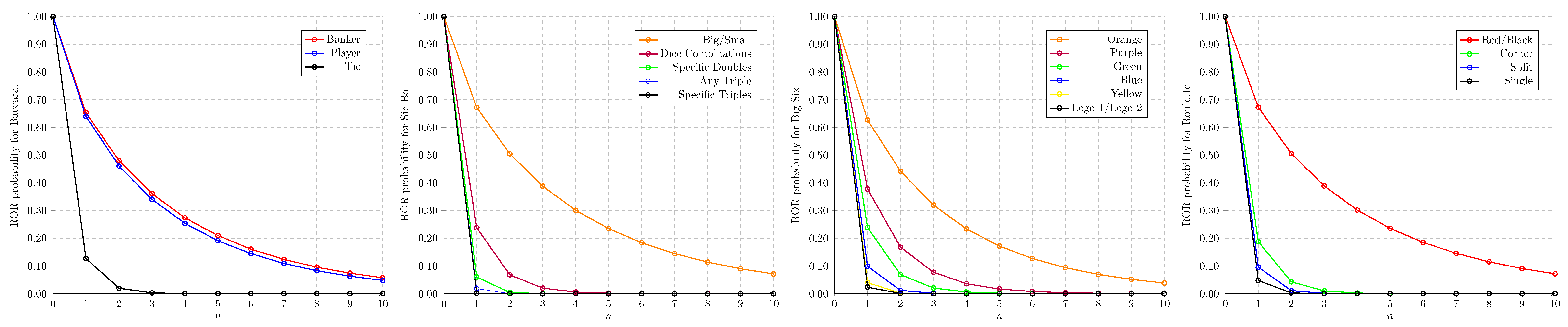
The following tables lay out our configurative setting and the corresponding evaluation outcomes of ROR probabilities. The official data are evaluated with $n=1,2,\cdots ,10$. Each table corresponds to a common casino game with a number of wagers, and the obtained outcomes of the evaluation using the proposed model.

As indicated from

Table 1. The ROR probability obtained by applying the proposed model to each wager of baccarat.

Wager	p	a	$\mathit{n}=1$	2	3	4	5	6	7	8	9	10
Banker	45.9%	1.06%	6.53 × 10−1	4.80 × 10−1	3.61 × 10−1	2.74 × 10−1	2.10 × 10−1	1.61 × 10−1	1.24 × 10−1	9.59 × 10−2	7.42 × 10−2	5.75 × 10−2
Player	44.6%	1.24%	6.40 × 10−1	4.61 × 10−1	3.41 × 10−1	2.54 × 10−1	1.91 × 10−1	1.45 × 10−1	1.09 × 10−1	8.31 × 10−2	6.32 × 10−2	4.81 × 10−2
Tie	9.5%	14.36%	1.27 × 10−1	2.00 × 10−2	3.26 × 10−3	5.43 × 10−4	9.18 × 10−5	1.57 × 10−5	2.74 × 10−6	4.85 × 10−7	8.74 × 10−8	1.61 × 10−8

,

Table 2. The ROR probability obtained by applying the proposed model to each wager of Sic Bo.

Wager	p	a	$\mathit{n}=1$	2	3	4	5	6	7	8	9	10
Big/Small	48.61%	2.78%	6.72 × 10−1	5.05 × 10−1	3.88 × 10−1	3.01 × 10−1	2.35 × 10−1	1.84 × 10−1	1.45 × 10−1	1.14 × 10−1	9.02 × 10−2	7.13 × 10−2
Dice Combinations	13.90%	2.8%	2.38 × 10−1	6.84 × 10−2	2.04 × 10−2	6.17 × 10−3	1.88 × 10−3	5.77 × 10−4	1.77 × 10−4	5.47 × 10−5	1.69 × 10−5	5.22 × 10−6
Specific Doubles	7.41%	33.3%	6.05 × 10−2	4.67 × 10−3	4.00 × 10−4	3.89 × 10−5	4.47 × 10−6	6.06 × 10−7	9.32 × 10−8	1.55 × 10−8	2.69 × 10−9	4.76 × 10−10
Any Triple	2.78%	30.6%	1.84 × 10−2	4.35 × 10−4	1.15 × 10−5	3.58 × 10−7	1.44 × 10−8	7.49 × 10−10	4.61 × 10−11	3.08 × 10−12	2.13 × 10−13	1.49 × 10−14
Specific Triples	0.46%	30.1%	1.82 × 10−3	4.24 × 10−6	1.12 × 10−8	4.05 × 10−11	2.57 × 10−13	2.44 × 10−15	<1.0 × 10−15	<1.0 × 10−15	<1.0 × 10−15	<1.0 × 10−15

,

Table 3. The ROR probability obtained by applying the proposed model to each wager of the Big Six.

Wager	p	a	$\mathit{n}=1$	2	3	4	5	6	7	8	9	10
Orange	46.15%	7.69%	6.27 × 10−1	4.42 × 10−1	3.20 × 10−1	2.34 × 10−1	1.72 × 10−1	1.27 × 10−1	9.40 × 10−2	6.98 × 10−2	5.19 × 10−2	3.87 × 10−2
Purple	25.08%	7.69%	3.78 × 10−1	1.68 × 10−1	7.76 × 10−2	3.63 × 10−2	1.71 × 10−2	8.08 × 10−3	3.84 × 10−3	1.83 × 10−3	8.75 × 10−4	4.19 × 10−4
Green	15.38%	7.69%	2.39 × 10−1	6.91 × 10−2	2.07 × 10−2	6.28 × 10−3	1.92 × 10−3	5.93 × 10−4	1.84 × 10−4	5.70 × 10−5	1.78 × 10−5	5.54 × 10−6
Blue	7.69%	15.38%	9.88 × 10−2	1.21 × 10−2	1.54 × 10−3	2.00 × 10−4	2.65 × 10−5	3.58 × 10−6	4.94 × 10−7	6.97 × 10−8	1.01 × 10−8	1.52 × 10−9
Yellow	3.85%	19.23%	4.03 × 10−2	2.03 × 10−3	1.08 × 10−4	5.91 × 10−6	3.38 × 10−7	2.04 × 10−8	1.33 × 10−9	9.39 × 10−11	7.25 × 10−12	6.04 × 10−13
Logo 1/Logo 2	1.92%	11.54%	2.41 × 10−2	7.21 × 10−4	2.25 × 10−5	7.18 × 10−7	2.31 × 10−8	7.56 × 10−10	2.50 × 10−11	8.42 × 10−13	2.90 × 10−14	<1.0 × 10−15

and

Table 4. The ROR probability obtained by applying the proposed model to each wager of roulette.

Wager	p	a	$\mathit{n}=1$	2	3	4	5	6	7	8	9	10
Red/Black	18/37	2.7%	6.73 × 10−1	5.06 × 10−1	3.89 × 10−1	3.02 × 10−1	2.36 × 10−1	1.85 × 10−1	1.46 × 10−1	1.15 × 10−1	9.09 × 10−2	7.20 × 10−2
Corner	4/37	2.7%	1.88 × 10−1	4.32 × 10−2	1.03 × 10−2	2.48 × 10−3	6.04 × 10−4	1.48 × 10−4	3.63 × 10−5	8.93 × 10−6	2.20 × 10−6	5.43 × 10−7
Split	2/37	2.7%	9.61 × 10−2	1.14 × 10−2	1.40 × 10−3	1.76 × 10−4	2.21 × 10−5	2.81 × 10−6	3.57 × 10−7	4.55 × 10−8	5.80 × 10−9	7.42 × 10−10
Single	1/37	2.7%	4.81 × 10−2	2.87 × 10−3	1.78 × 10−4	1.12 × 10−5	7.15 × 10−7	4.57 × 10−8	2.93 × 10−9	1.88 × 10−10	1.21 × 10−11	7.80 × 10−13

and Figure 1, in general, ROR probabilities keep decreasing as n increases, which is coherent with the conclusion of Theorem 1. Further, the smaller the value of p, the higher the decreasing rate of the ROR probability. Interestingly, when $n=1$, the ROR probability is even higher than p (the probability of the casino winning). This situation lasts until $n\ge 3$. Thus, despite the fact that $50\%<p<100\%$, casinos are still able to lower the risk of bankruptcy through controlling n. Take the casino game baccarat, for example. Referring to the p and a in Table 1, when $n=100$, the proposed model indicates that the $\mathit{Pro}\left(100\right)$ values of betting on banker and player are 1.25 × 10⁻¹¹ and 2.21 × 10⁻¹², respectively, which implies that no one could bankrupt the casino even if the global population had participated in the game. Based on $n=⌊\frac{\mathit{Bankroll}}{\mathit{MaxBet}}⌋$, once the casino ensures its operating bankroll to be larger than $n\times \mathit{MaxBet}$, the risk of bankruptcy is negligible.

It is worth mentioning that blackjack and Pai Gow fall into the category of skill games, in which p varies based on players’ decisions and strategies. Take blackjack, for example. Players can enjoy a house advantage as low as 0.5% if they employ the basic strategy, while players with poor skill can suffer with a much higher one, e.g., 4.0%. In the extreme case ($p=1.0$) indicated in the last paragraph of Section 3, the casino is confronted by a challenge of bankruptcy. Unfortunately, this extreme case could possibly emerge, as some gamblers with sophisticated skill in card counting, or those who cheat with some equipment in practising advantage plays, could beat the casino and at least force p to get very close to $1.0$. Of course, casinos counter these kinds of practice with some protection measures, such as reinforcing surveillance capabilities, using eight-deck cards and others, in the hope of dragging p back to the normality of the model. The proposed model also tells us that even though $p=1.0$ emerges, the gambler still has to go through at least n games to bankrupt the casino. Therefore, the casino must set up a proper $\mathit{MaxBet}$ to adjust n, which allows surveillance personnel ample time to find the frauds, if any.

However, no matter how small the chance is, Murphy’s Law suggests that the possibility of bankruptcy might be more likely than we thought. Based on the underlying assumption of the proposed model, the gambler has unlimited credits. In practice, casinos keep operating for a certain period time and have supposedly accumulated a larger bankroll due to the fact of favourable house advantages, implying a larger n. Based on Theorem 1, the larger the value of n, the lower the risk of bankruptcy. Thus, the worry from Murphy’s Law could somewhat subside.

4.2. Evaluation and Discussion

We used the collected settings to perform predictions on other ROR models and compared the results with our proposed model for analysis. The selected benchmark ROR approaches were the Coolidge [8], Kaufmann [33] and Ralph-Vince [34] formulas and the negative binomial regression model (NBRM) [35]. We also provide the results of our proposed model without considering the house advantage ($a=0.0$). The $n=10$ of various formulas can also be regarded as the extent of the risk that the casino can assume before reaching the bankruptcy threshold.

For the Coolidge model, it uses the same independent control variables as the Kaufmann and Ralph-Vince formulas, and the dependent variables (p and current win rate) have been described by a more reasonable ordinal model. Similar to the model we proposed, we expanded their concept and took account of the house advantage instead of the current winning percentage. The probability of winning and the bankroll or budget as factors are regarded as the input features (independent variables) each formula must receive. In our empirical simulation, Coolidge provides the roughest prediction, in which it only considers a without p, because it is believed that a and p can be derived directly from each other. They do not have to be used as different input variables, so their results can only reflect very simple situations with a lack of clarity. In contrast, the Kaufmann and Ralph-Vince methods provide us with more accurate results than Coolidge. They analyse the probability of winning and take the risk percentage into their consideration, but it is still not perfect, because the risk percentage requires the size of the risk/return and the win rate, which will change from time to time and is actually not suitable for ROR estimation. However, in reality, instead of predicting the casino’s current ratio of wins and losses, it is better to consider the ROR prediction in the next n rounds. Taking these factors into account can make the formula very complicated, and this is where the model based on Poisson distribution comes into play. It is noted here that when comparing the performance of different models, we should not incorporate the casino profit ($n\times a$) into the NBRM model. This is mainly because the model is a counting model and is usually designed to model interval-scale data rather than ordinal-scale data. Furthermore, unlike a and p features, the risk percentage varies from person to person and does not affect the ROR. Instead, the risk percentage usually influences the gambler’s betting behaviour and indirectly affects $\mathit{MaxBet}$. As a result, it is not reasonable to directly incorporate this information into NBRM and our proposed model.

Table 5. ROR probabilities estimated by different models. Please refer to the above tables for variable configurations.

Game and Its Wager		Coolidge	Kaufmann	Ralph-Vince	NBRM	Equation (7)	Equation (8)
Baccarat	Banker	4.74 × 10−1	7.87 × 10−3	6.13 × 10−2	6.42 × 10−2	6.18 × 10−2	5.75 × 10−2
	Player	4.69 × 10−1	6.78 × 10−3	5.54 × 10−2	6.13 × 10−2	5.25 × 10−2	4.81 × 10−2
	Tie	2.07 × 10−1	6.18 × 10−6	4.76 × 10−4	2.14 × 10−7	3.03 × 10−7	1.61 × 10−8
Sic Bo	Big/Small	4.32 × 10−1	1.06 × 10−2	7.52 × 10−2	6.81 × 10−2	8.46 × 10−2	7.13 × 10−2
	Dice Combinations	4.31 × 10−1	3.11 × 10−5	1.43 × 10−3	2.59 × 10−6	8.88 × 10−6	5.22 × 10−6
	Specific Doubles	5.34 × 10−2	2.19 × 10−6	2.35 × 10−4	1.87 × 10−8	3.10 × 10−8	4.76 × 10−10
	Any Triple	6.48 × 10−2	3.95 × 10−8	1.54 × 10−5	8.45 × 10−11	2.70 × 10−12	1.49 × 10−14
	Specific Triples	6.71 × 10−2	2.82 × 10−11	1.12 × 10−7	5.09 × 10−12	<1.0 × 10−15	<1.0 × 10−15
Big Six	Orange	3.23 × 10−1	8.10 × 10−3	6.25 × 10−2	6.13 × 10−2	6.37 × 10−2	3.87 × 10−2
	Purple	3.23 × 10−1	4.23 × 10−4	8.41 × 10−3	1.82 × 10−3	1.09 × 10−3	4.19 × 10−4
	Green	3.23 × 10−1	4.82 × 10−5	1.92 × 10−3	2.91 × 10−5	2.11 × 10−5	5.54 × 10−6
	Blue	1.93 × 10−1	2.56 × 10−6	2.61 × 10−4	1.82 × 10−9	4.37 × 10−8	1.52 × 10−9
	Yellow	1.47 × 10−1	1.48 × 10−7	3.78 × 10−5	1.07 × 10−12	6.30 × 10−11	6.04 × 10−13
	Logo 1/Logo 2	2.51 × 10−1	8.83 × 10−9	5.55 × 10−6	4.94 × 10−13	7.26 × 10−14	<1.0 × 10−15
Roulette	Red/Black	4.34 × 10−1	1.07 × 10−2	7.54 × 10−2	6.63 × 10−2	8.50 × 10−2	7.20 × 10−2
	Corner	4.34 × 10−1	1.07 × 10−5	6.90 × 10−4	2.22 × 10−8	9.72 × 10−7	5.43 × 10−7
	Split	4.34 × 10−1	5.95 × 10−7	9.71 × 10−5	1.55 × 10−10	1.61 × 10−9	7.42 × 10−10
	Single	4.34 × 10−1	3.52 × 10−8	1.42 × 10−5	8.65 × 10−13	2.05 × 10−12	7.80 × 10−13

illustrates the estimates of the benchmark models and our proposed model with and without house advantage consideration. In addition to Coolidge, most of the results indicate the expected performance. In summary, all models present roughly the same situation: The derivative signs of the control variables (p and a) are basically the same in all of these models (the greater the value of p, the greater the ROR caused by $\frac{\partial }{\partial p}\mathit{Pro}\left(n\right)>0$, but the larger the value of a, the smaller the ROR caused by $\frac{\partial }{\partial a}\mathit{Pro}\left(n\right)<0$). Among all the methods, the Coolidge results are biased toward conservative, rendering higher probabilities of ruin even when the gamblers’ win rates are low. Take Sic Bo’s Specific Triples as an example. While $p=0.46\%$, its ROR still reaches 6.71 × 10⁻². Compared to Kaufmann and Ralph-Vince, Coolidge’s results are more comprehensive and more readily identifiable. However, this method is still not perfect because the current number of wins/losses must be calculated before predictions can be made due to different outcomes being generated each time. Another limitation is that the upper bound of n is required to be defined, which is obviously not feasible in practice. Furthermore, the results produced by NBRM are similar to the proposed model, which is similar to Equation (7) except for taking the house advantage (a) into consideration. This is because they also make use of the binomial distribution in the derivation process: The NBRM focuses on the binomial distribution of a finite sample and the proposed model is conducted to describe the distribution from an infinite sample, thereby giving the probability of obtaining the entire event in the population. In addition, the ruin prediction can be further alleviated when considering the impact of profit ($a>0$). In fact, the simulated outcomes generated through these models are quite well understood and these models can roughly determine how each input feature influences the outcomes. We put forth the mathematical model that merely links up their relationship and describes how these changes affect the ROR through mathematical proof.

5. Risk of Ruin Scales

In terms of application, we want to provide an ROR measurement standard so that users can directly specify the current risk level of certain game settings. In order to produce a practical formula to obtain some useful measures, we carried out the calculations with the following required features:

• The ROR measurement must be able to support high-precision decimals because it will receive the probability of ROR by $\mathit{Pro}\left(n\right)$.
• Minimum and maximum values should be determined in order to normalise the ROR measurement.
• Certainly, the maximum risk must be obtained when the input is 1.0.
• There exists a small deviation that can be negligible for approximating the limit of risk.

In response to the above requirements and based on our simulation results, we make use of the logarithmic scaling function to analyse the ROR probability through $\mathit{ROR}\left(x\right)$ as follows:

$$\mathit{ROR}\left(x\right)=logx-logS=log\frac{x}{S}$$

(11)

Here, S is equal to 1.0 × 10⁻¹⁰ as a sufficiently small value for delimiting. The input x is the predicted risk probability based on the proposed model. Since we are using a logarithmic scale that can represent the index of high-precision values, each step is spaced with a tenfold increase in probability. If $x=1.0$ is input, the result of Equation (11) will be equal to $10.0$, representing the maximum risk, and if $x\le S$, the result is less than or equal to $0.0$, representing the minimum/no risk.

Based on the scales specified in

Table 6. A description of $\mathit{ROR}\left(x\right)$ according to the world’s population.

Scale	Status	One Out of the Number of People That Can Bankrupt the Casino by the Same Game
$\le 1.25$	SAFE	The casino cannot be bankrupted even against the world’s population
$\left(1.25,2.50\right]$	RELAXED	Approx. 600 million people (half the size of China’s population)
$\left(2.50,3.75\right]$	RISKY	Approx. 30 million people (the size of a small- to mid-sized province in China in terms of population)
$\left(3.75,5.00\right]$		Approx. 1,750,000 people (the size of a small- to mid-sized city in terms of population)
$\left(5.00,6.25\right]$	DANGEROUS	Approx. 100,000 people
$\left(6.25,7.50\right]$		Approx. 5000 people
$\left(7.50,8.75\right]$	RUINED	Everyone could bankrupt the casino
$\left(8.75,10.0\right]$		Casinos can be considered bankrupt

, the scales Dangerous and Ruined should not be allowed to appear in the perspective of casinos, in which casinos could possibly go bankrupt within a month, particularly as per the gambling behaviour of Chinese people. Corresponding to Table 3, we can apply Equation (11) to the ROR probabilities generated by the Big Six game.

As indicated in

Table 7. Proposed ROR scales for the Big Six.

Wager	p	a	$\mathit{n}=1$	2	3	4	5	6	7	8	9	10
Orange	46.15%	7.69%	9.80	9.65	9.51	9.37	9.24	9.10	8.97	8.84	8.72	8.59
Purple	25.08%	7.69%	9.58	9.23	8.89	8.56	8.23	7.91	7.58	7.26	6.94	6.62
Green	15.38%	7.69%	9.38	8.84	8.32	7.80	7.28	6.77	6.26	5.76	5.25	4.74
Blue	7.69%	15.38%	8.99	8.08	7.19	6.30	5.42	4.55	3.69	2.84	2.00	1.18
Yellow	3.85%	19.23%	8.61	7.31	6.03	4.77	3.53	2.31	1.12	<0.0	<0.0	<0.0
Logo 1/Logo 2	1.92%	11.54%	8.38	6.86	5.35	3.86	2.36	0.88	<0.0	<0.0	<0.0	<0.0

, the casino will stay in a status of Ruined no matter which wager is selected if $n<2$. Therefore, the casino must avoid falling into this status. As stated above, $\mathit{ROR}\left(x\right)$ in Equation (11) changes based on $\mathit{Pro}\left(n\right)$, and $\mathit{Pro}\left(n\right)$ in Equation (10) is derived from the three determinants n, p and a. Thus, adjustments can be made through adjusting the three factors. However, p is an inherent probability of a specific non-skill game and apparently cannot be changed at will. a is derived from p and a payout ratio determined by the casino, and the payout ratio is strictly regulated by governments, hence the span of adjustment is surely very limited in lowering ROR scales. Finally, n is left as the only option for adjustment. n can be considered as $⌊\frac{\mathit{Bankroll}}{\mathit{MaxBet}}⌋$, such that the casino can increase n by lowering the $\mathit{MaxBet}$, or increasing the size of the bankroll. Take the Big Six’s Orange as an example. Table 7 only lists the cases of $n=1\cdots 10$ and all of them result in a RUINED status. In subsequent cases, when $n=20$, the risk of ruin is mitigated to $7.33$ (DANGEROUS) and is further lowered to $4.92$ (RISKY) when $n=40$. Finally, when $n>60$, the risk reaches RELAXED status or lower. In summary, a casino can run its business free of worry of bankruptcy if the $\mathit{MaxBet}$ for each wager has also been configured to acceptably low levels.

6. Conclusions

In this study, we presented a novel model for predicting the ROR with higher precision by using Poisson distribution theory, from pre-defined sets of factors: the win probability (p), the house advantage (a), and the predicted maximum number of bets (n). We have given the complete derivation procedure that leads to the formal justification and the algorithm, which satisfies monotonicity and contains probabilistic features. This research fills the current research gap by exploring the relationship between the cash flow and the max limit of betting in the model, and examining how they interact to affect the bankruptcy risk of the casino. On the basis of risk awareness and social support theories, we developed a comprehensive typological ROR scale measure, which can help eliminate the need for heavy mathematics for ROR model derivation. Then, we summarised the status that reflects the scale of the ROR, which can clearly describe the impact of the casino’s current settings on its bankruptcy risk, implying that the casino needs to take risks although house advantages favour them. In practice, this research provides useful information for managing each gamble so that high-risk settings can be discovered in time. In addition, we show that the proposed model and measure have the potential to facilitate related applications and analysis.

Further, from the perspective of responsible gaming advocacy, these results were devised in a form that effectively delivers visualized and concrete hints to those gamblers who are susceptible to developing problem-gambling behaviour, by arousing their rationality to be disillusioned with their false hope and myths. Particularly, those who strongly believe in their so-called formulas for beating casinos are among the problem gamblers who fall prey to unhealthy gambling habits. Furthermore, casinos typically have a much larger bankroll with respect to general individual gamblers, which poses a further disadvantage to them. As our tabulated results concretely and concisely show, the longer the string of bets the gamblers place, the higher the chance casinos will win. In this zero-sum game, the advantage is definitely not on the gamblers’ side.

References

1. Siu, K.M.; Hoi, L.M.; Chan, K.H. A Proposed Set of Features on Implementing Responsible Gambling on Slot Games with G2S Technology. In Proceedings of the 2021 International Conference on Computer Science and Engineering (IC2SE), Padang, Indonesia, 16 November 2021. [Google Scholar] [CrossRef]
2. Cai, X. The House Edge and the Basic Strategy of Blackjack. SHS Web Conf. 2022, 148, 03038. [Google Scholar] [CrossRef]
3. Newall, P.W.S.; Walasek, L.; Ludvig, E.A. Risk communication improvements for gambling: House-edge information and volatility statements. Psychol. Addict. Behav. 2022, 36, 358–363. [Google Scholar] [CrossRef]
4. Hales, C.; Clark, L.; Winstanley, C. Computational approaches to modeling gambling behaviour: Opportunities for understanding disordered gambling. Neurosci. Biobehav. Rev. 2023, 147, 105083. [Google Scholar] [CrossRef]
5. Siu, K.M.; Lei, I.S. Principles of Gaming Technologies; Mcgraw Hill Education: Singapore, 2020. [Google Scholar]
6. Hannum, R.C.; Cabot, A.N. Practical Casino Math; Trace Publication: Dallas, TX, USA, 2005; p. 300. [Google Scholar]
7. Cabot, A.; Hannum, R.C. Practical Casino Math; Institute for the Study of Gambling and Commercial Gambling: Macau, China, 2002; p. 247. [Google Scholar]
8. Coolidge, J.L. The Gambler’s Ruin. Ann. Math. 1909, 10, 181. [Google Scholar] [CrossRef]
9. Woolley, R.; Livingstone, C.; Harrigan, K.; Rintoul, A. House edge: Hold percentage and the cost of EGM gambling. Int. Gambl. Stud. 2013, 13, 388–402. [Google Scholar] [CrossRef]
10. Dubins, L.E. How to Gamble If You Must Inequalities for Stochastic Processes; Dover Publications: Mineola, NY, USA, 2014; p. 274. [Google Scholar]
11. Picard, P.; Lefèvre, C. The probability of ruin in finite time with discrete claim size distribution. Scand. Actuar. J. 1997, 1997, 58–69. [Google Scholar] [CrossRef]
12. Li, J.; Tang, Q.; Wu, R. Subexponential tails of discounted aggregate claims in a time-dependent renewal risk model. Adv. Appl. Probab. 2010, 42, 1126–1146. [Google Scholar] [CrossRef] [Green Version]
13. Leipus, R.; Šiaulys, J. Finite-horizon ruin probability asymptotics in the compound discrete-time risk model. Lith. Math. J. 2011, 51, 207–219. [Google Scholar] [CrossRef]
14. Thorin, O. Some Comments on the Sparre Andersen Model in the Risk Theory. ASTIN Bull. 1974, 8, 104–125. [Google Scholar] [CrossRef] [Green Version]
15. Cheng, D.; Yu, C. Uniform asymptotics for the ruin probabilities in a bidimensional renewal risk model with strongly subexponential claims. Stochastics Int. J. Probab. Stoch. Process. 2018, 91, 643–656. [Google Scholar] [CrossRef]
16. Choi, K.C.; Li, S.; Lam, C.T.; Wong, A.; Lei, P.; Ng, B.; Siu, K.M. Genetic Algorithm For Tourism Route Planning Considering Time Constrains. Int. J. Eng. Trends Technol. 2022, 70, 171–179. [Google Scholar] [CrossRef]
17. Afonso, L.B.; Cardoso, R.M.R.; dos Reis, A.D.E.; Guerreiro, G.R. Ruin Probabilities And Capital Requirement for Open Automobile Portfolios With a Bonus-Malus System Based on Claim Counts. J. Risk Insur. 2019, 87, 501–522. [Google Scholar] [CrossRef]
18. Winstanley, C.A.; Clark, L. Translational Models of Gambling-Related Decision-Making. In Translational Neuropsychopharmacology; Springer International Publishing: Berlin/Heidelberg, Germany, 2015; pp. 93–120. [Google Scholar] [CrossRef]
19. Li, B.; Ni, W.; Constantinescu, C. Risk models with premiums adjusted to claims number. Insur. Math. Econ. 2015, 65, 94–102. [Google Scholar] [CrossRef]
20. Jewell, W. Bayesian Regression and Credibility Theory; Iiasa Research Memorandum; IIASA: Laxenburg, Austria, 1975. [Google Scholar]
21. Asmussen, S.; Biard, R. Ruin probabilities for a regenerative Poisson gap generated risk process. Eur. Actuar. J. 2011, 1, 3–22. [Google Scholar] [CrossRef] [Green Version]
22. Constantinescu, C.; Dai, S.; Ni, W.; Palmowski, Z. Ruin Probabilities with Dependence on the Number of Claims within a Fixed Time Window. Risks 2016, 4, 17. [Google Scholar] [CrossRef] [Green Version]
23. Afonso, L.B.; Cardoso, R.M.R.; dos Reis, A.D.E.; Guerreiro, G.R. Measuring the Impact of a Bonus-Malus System in Finite and Continuous Time Ruin Probabilities for Large Portfolios in Motor Insurance. ASTIN Bull. 2017, 47, 417–435. [Google Scholar] [CrossRef]
24. Wagner, C. Time in the red in a two state Markov model. Insur. Math. Econ. 2002, 31, 365–372. [Google Scholar] [CrossRef]
25. Willmot, G.E. Refinements and distributional generalizations of Lundberg’s inequality. Insur. Math. Econ. 1994, 15, 49–63. [Google Scholar] [CrossRef]
26. Lu, Y.; Chen, G.; Yin, Q.; Sun, H.; Hou, M. Solving the ruin probabilities of some risk models with Legendre neural network algorithm. Digit. Signal Process. 2020, 99, 102634. [Google Scholar] [CrossRef]
27. Chan, K.H.; Ke, W.; Im, S.K. A General Method for Generating Discrete Orthogonal Matrices. IEEE Access 2021, 9, 120380–120391. [Google Scholar] [CrossRef]
28. Chan, S.; Dillon, T.; Siu, A. Applying a mediator architecture employing XML to retailing inventory control. J. Syst. Softw. 2002, 60, 239–248. [Google Scholar] [CrossRef]
29. Lam, C.S.; Greenlees, M. Casino money laundering regulations—Macao and USA. J. Money Laund. Control 2017, 20, 52–69. [Google Scholar] [CrossRef]
30. Godinho, J. Casino Gaming in Macau: Evolution, Regulation and Challenges. UNLV Gaming Law J. 2014, 5, 7. [Google Scholar]
31. Buhi, J. Corporate Social Responsibility, Casino Capitalism, and the Constitution of Macau. UCLA Pac. Basin Law J. 2020, 37, 1–23. [Google Scholar] [CrossRef]
32. Siu, K.M.; Chan, K.H.; Im, S.K. The Evolution and Practices of Current IT Management with a Focus on Applications with Data Management. In Proceedings of the 2022 IEEE 5th International Conference on Computer and Communication Engineering Technology (CCET), Beijing, China, 19–21 August 2022. [Google Scholar] [CrossRef]
33. Kaufman, P.J. Smarter Trading; McGraw: New York, NY, USA, 1994; p. 244. [Google Scholar]
34. Vince, R. Portfolio Management Formulas; Wiley: Hoboken, NJ, USA, 1990; p. 253. [Google Scholar]
35. Hilbe, J.M. Negative Binomial Regression; Cambridge University Press: Cambridge, UK, 2011. [Google Scholar] [CrossRef]
Figure 1. The ROR probability of various gambling methods predicted by the proposed model.
Mathematics 11 01736 g001