
Managing Disruptions in a Flow-Shop Manufacturing System
 , ,
, ,
Abstract
1. Introduction
2. Background Review
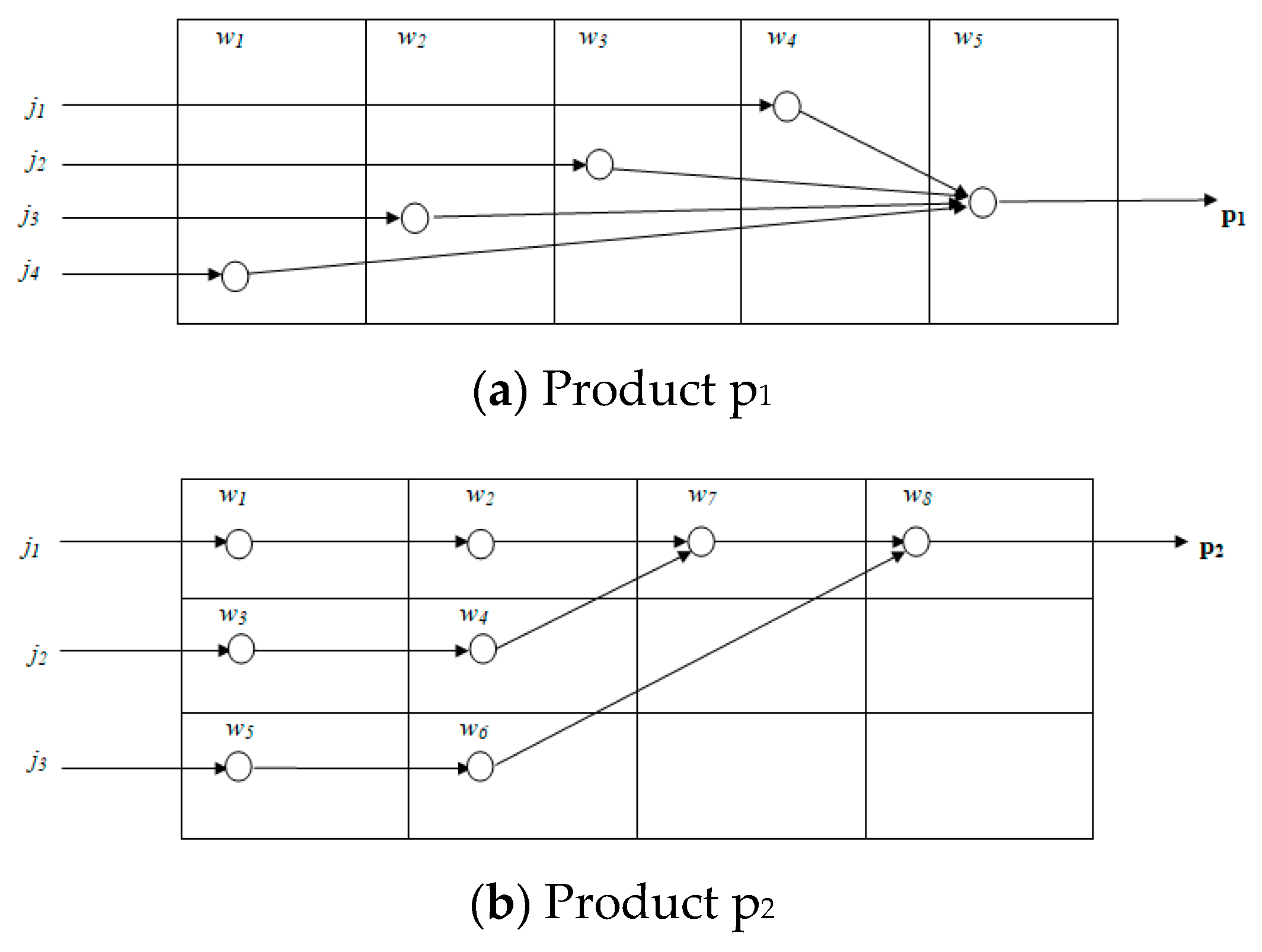
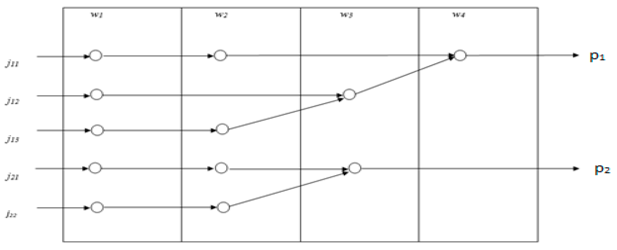
3. Problem on Hand: Flow-Shop with Assembly Operation
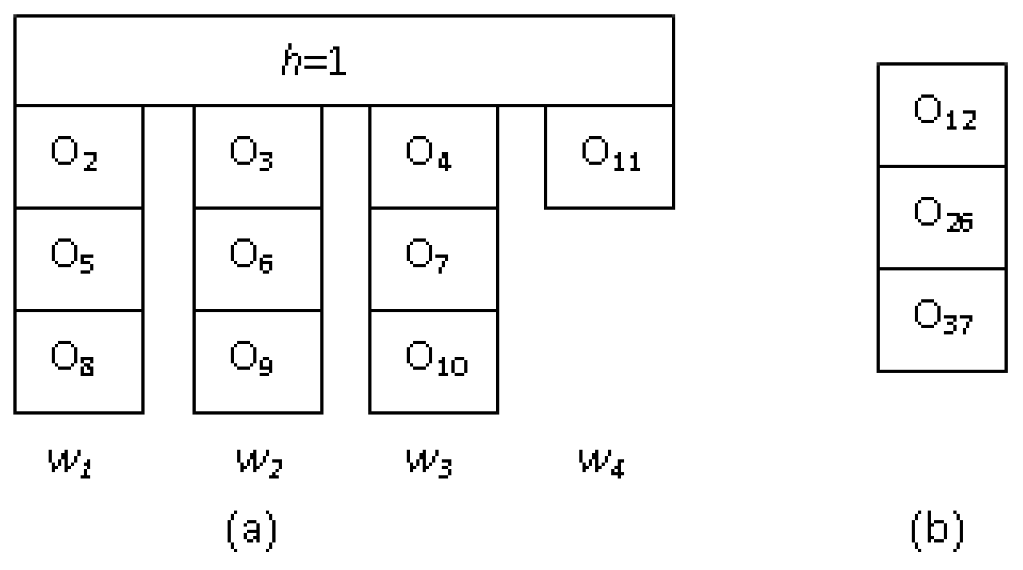
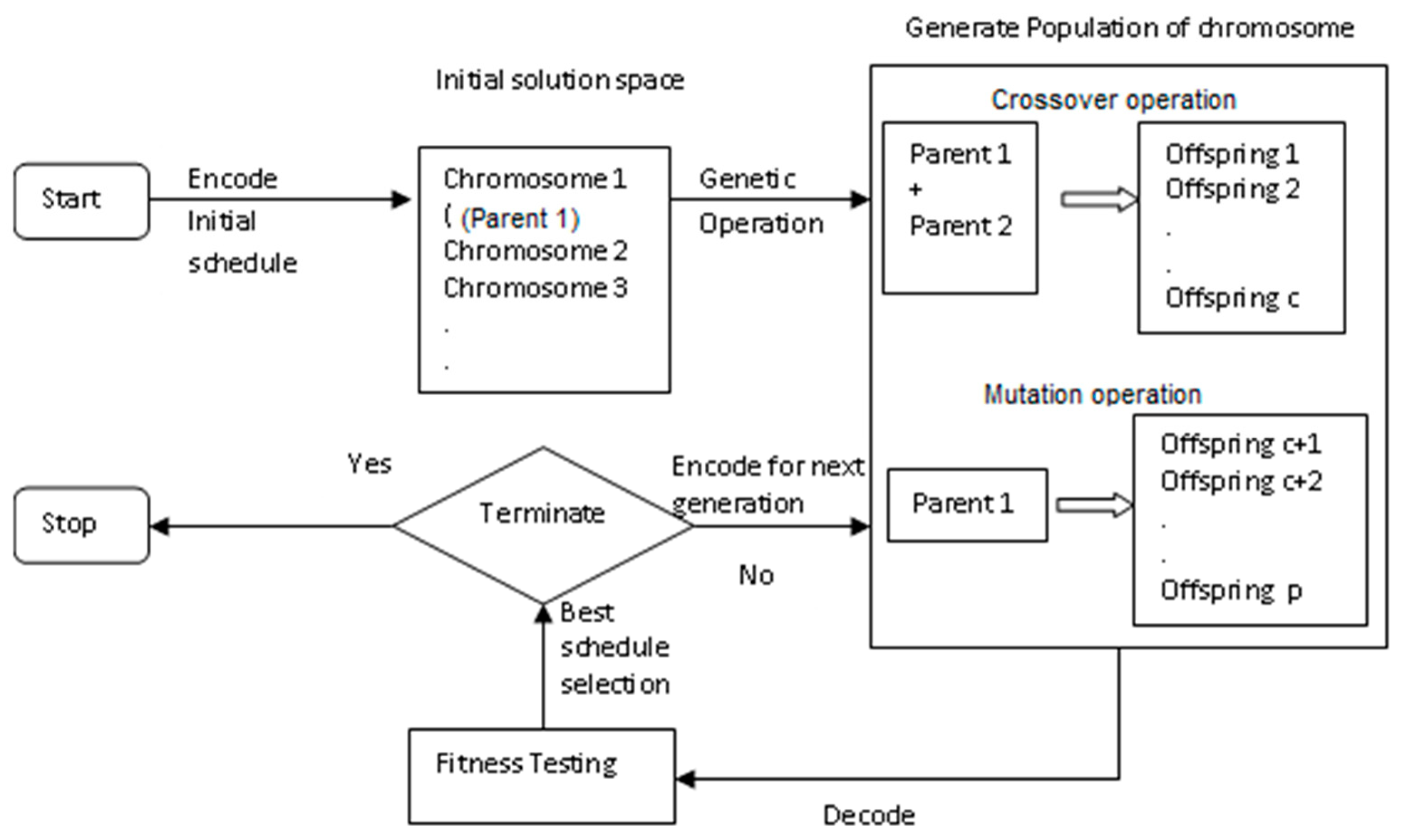
3.1. Genetic Algorithm
3.2. Modified Bottleneck Minimal Idleness
4. Proposed Approach
4.1. Right-Shift Rescheduling (RSR)
4.2. Break down Machine Heuristics
4.3. Use of Genetic Algorithm
- Each part can handle up to one workstation at a time. All parts are stand-alone, available for zero-time processing, and may or may not require all workstations.
- A workstation is continuously available and processes parts in the same order; for example, if part jhi is processed on a workstation before part jhi+1, then all workstations proceed in the same way.
- Setup times for the parts and assemblies are negligible and therefore ignored.
- It is permissible to keep inventory during the process.
- Transit time is zero, which makes a part available on a workstation wj+1 as soon as it leaves workstation wj.
- All products have the same delivery dates.
- All the parts and machines immediately resume their execution once the reschedule is made available.
- The duration of the breakdown is known as soon as it occurs.
- A machining workstation other than the first fails in a random manner.
- After rescheduling, an interrupted, incomplete operation, if any, will be completed on the same machine.
- Disruption occurs only at machining workstations. Disruption at assembly workstations is assumed to be negligible as the number of operations at these workstations is less than those at machining workstations.
5. Performance of Rescheduling: Design of Experiments
6. Discussion and Interpretation of Results
7. Conclusions
Author Contributions
Funding
Institutional Review Board Statement
Informed Consent Statement
Data Availability Statement
Acknowledgments
Conflicts of Interest
Appendix A

| Ref. | Initial Schedule | Rescheduling Strategy * | Performance Measure | Disruptions ** | Production System | Findings/Remarks |
|---|---|---|---|---|---|---|
| [14] | Nominal | AOR | Flow time, tardiness, and machine utilization | MF, NJ, JC, urgent job | Flexible manufacturing system (FMS) | Shortlisted dispatching rules performed better than the early due date for rescheduling |
| [15] | Nominal | RSR/AOR/TR | Efficiency and stability | MF | Job-shop | AOR demonstrated superior performance over all other methods in most situations |
| [16] | Nominal | RSR/AOR | Earliness, tardiness, and stability | MF | Flow-shop | Used the embedded dominance rule for rescheduling |
| [17] | Nominal | AOR | Robustness | MF | Flow-shop | Determined trigger value for deciding rescheduling |
| [18] | Nominal | AOR | Machine utilization, setup, and rescheduling frequency | MF | Parallel machine | Used periodic, event-driven, and hybrid rescheduling strategies |
| [19] | Normal | AOR | Tardiness | MF, NJ, JC | Job-shop FMS | An adaptive genetic algorithm is applied |
| [20] | Nominal | RSR/AOR | Make-span and deviation of the start times | MF, NJ, PT vary, urgent job | Job-shop | AOR performed better. Experimented with up to 500 operations for various sizes and incidences of disruptions |
| [21] | Nominal | RSR/AOR/TR | Total weighted tardiness | MF | Job-shop | TR outperformed other methods. Used a modified shifting bottleneck method for scheduling and rescheduling. |
| [22] | No schedule | AOR | make-span, tardiness, and start time deviation | NJ | Job-shop | Used the genetic local search method for periodic rescheduling |
| [23] | Nominal | AOR | Total flow time and number of disrupted jobs | MF | Parallel machine | Used the shortest processing time for rescheduling |
| [24] | Nominal | AOR | Cost deviation related to part and machine preparation | MF, NJ | FMS/Job-shop | Used an agent-based approach |
| [25] | Dispatching rule | RSR/AOR | Tardiness and degree of similarity | MF | Job-shop | The proposed method of message passing and the local search algorithm performed well |
| [26] | Normal | AOR | Efficiency | NJ | Job-shop | Genetic algorithm-based reactive scheduling |
| [27] | Robust | RSR | Robustness and deviation of completion times | MF | Single machine | Applied to the predictive schedule |
| [28] | Nominal | RSR AOR | Make-span and lateness | NJ, delay in processing time | Flow-shop with parallel machines | Initial schedule was generated with a commercial constraint programming solver and a low impact rescheduling algorithm was proposed |
| [29] | Nominal | RSR AOR | Earliness, tardiness, and cost and deviation of completion time | MF | Parallel machine | A linear programming model for scheduling and a minimum-cost network flow algorithm were used for reactive scheduling. |
| [30] | Nominal | AOR | Flowtime and stability in tooling cost | MF | Unrelated parallel machines | Used algorithms by incorporating powerful reduction and bounding mechanisms |
| [31] | Nominal | AOR | Tardiness, flowtime, and make-span and stability in start times | MF | Job-shop | Dispatching rules generated an initial schedule |
| [32] | Nominal | AOR/RSR | Tardiness, number of tardy jobs, setup time, total idle time of machines, total flow time, start time deviation, and change in operations sequence | NJ | Job-shop | The match-up algorithms proposed performed well |
| [33] | Normal | AOR | Make-span and tardiness, start time and process sequence deviation, and change in machine allocation | NJ | FMS | A genetic algorithm was proposed for match up scheduling with a non-reshuffle strategy and performed better than the reshuffle and TR methods |
| [34] | Nominal | RSR AOR TR | Make-span and deviation of the start times | MF, NJ, Job ready time variation | Flow-shop | An iterated greedy algorithm was used for predictive and reactive scheduling. It performed better than the local search and repair method |
| [35] | Nominal | RSR/AOR | No. of disrupted jobs and cost due to additional resources | MF | Unidentical parallel machines | Heuristics for the initial schedule and improvement used the local search algorithm |
| [36] | Normal | Periodic/event driven | Make-span, tardiness, and start time deviation, and cost | NJ | Job-shop | A non-dominated sorting algorithm was used. Length of the scheduling interval, no. of jobs added, and shop utilization showed influence on efficiency measures |
| [37] | Normal | AOR | Make-span and energy consumption | Job-shop | Applied match-up and memetic algorithms in a sustainable environment | |
| [38] | Normal | AOR/RSR | Equipment utilization and degree of similarity | MF | Job-shop with parallel machines | The concept of match-up scheduling was used for single and group machines, for partial repair of affected segment(s) of the schedule |
| [39] | Normal | Selection from trained data | Tardiness | NJ | Job-shop | The knowledge gathered with the deep learning reinforcement method was used for the optimal sequence and repair of operations |
| [40] | Normal | AOR | Make-span and deviation of no. of job allocations | Hybrid flow-shop | A multi-objective evolutionary algorithm was employed | |
| [41] | Normal | RSR/AOR | Make-span, computational time, energy consumption, and setup time | MF | Unidentical parallel machines | Used greedy heuristics and metaheuristics |
| [42] | Normal | Simulation | Delivery due dates | Change in delivery plan | Hybrid flow-shop | Multimethod modeling was used, which involved simulation of interacting agents with any logic software |
| [43] | Nominal | Simulation | Make-span and completion time | MF | Assembly flow-shop | Used an adaptive evolutionary algorithm on a two-stage assembly flow-shop scheduling problem with random breakdowns |
Appendix B
| # | F1 $ | F2 | F3 | F4 | F5 | F6 | # | F1 | F2 | F3 | F4 | F5 | F6 | # | F1 | F2 | F3 | F4 | F5 | F6 | # | F1 | F2 | F3 | F4 | F5 | F6 |
|---|---|---|---|---|---|---|---|---|---|---|---|---|---|---|---|---|---|---|---|---|---|---|---|---|---|---|---|
| 1 | 1 | 1 | 1 | 1 | 1 | 1 | 25 | 1 | 2 | 1 | 1 | 1 | 2 | 49 | 2 | 1 | 1 | 1 | 1 | 1 | 73 | 2 | 2 | 1 | 1 | 1 | 2 |
| 2 | 1 | 1 | 2 | 1 | 1 | 1 | 26 | 1 | 2 | 2 | 1 | 1 | 2 | 50 | 2 | 1 | 2 | 1 | 1 | 1 | 74 | 2 | 2 | 2 | 1 | 1 | 2 |
| 3 | 1 | 1 | 1 | 1 | 2 | 1 | 27 | 1 | 2 | 1 | 1 | 2 | 2 | 51 | 2 | 1 | 1 | 1 | 2 | 1 | 75 | 2 | 2 | 1 | 1 | 2 | 2 |
| 4 | 1 | 1 | 2 | 1 | 2 | 1 | 28 | 1 | 2 | 2 | 1 | 2 | 2 | 52 | 2 | 1 | 2 | 1 | 2 | 1 | 76 | 2 | 2 | 2 | 1 | 2 | 2 |
| 5 | 1 | 1 | 1 | 2 | 1 | 1 | 29 | 1 | 2 | 1 | 2 | 1 | 2 | 53 | 2 | 1 | 1 | 2 | 1 | 1 | 77 | 2 | 2 | 1 | 2 | 1 | 2 |
| 6 | 1 | 1 | 2 | 2 | 1 | 1 | 30 | 1 | 2 | 2 | 2 | 1 | 2 | 54 | 2 | 1 | 2 | 2 | 1 | 1 | 78 | 2 | 2 | 2 | 2 | 1 | 2 |
| 7 | 1 | 1 | 1 | 2 | 2 | 1 | 31 | 1 | 2 | 1 | 2 | 2 | 2 | 55 | 2 | 1 | 1 | 2 | 2 | 1 | 79 | 2 | 2 | 1 | 2 | 2 | 2 |
| 8 | 1 | 1 | 2 | 2 | 2 | 1 | 32 | 1 | 2 | 2 | 2 | 2 | 2 | 56 | 2 | 1 | 2 | 2 | 2 | 1 | 80 | 2 | 2 | 2 | 2 | 2 | 2 |
| 9 | 1 | 2 | 1 | 1 | 1 | 1 | 33 | 1 | 1 | 1 | 1 | 1 | 3 | 57 | 2 | 2 | 1 | 1 | 1 | 1 | 81 | 2 | 1 | 1 | 1 | 1 | 3 |
| 10 | 1 | 2 | 2 | 1 | 1 | 1 | 34 | 1 | 1 | 2 | 1 | 1 | 3 | 58 | 2 | 2 | 2 | 1 | 1 | 1 | 82 | 2 | 1 | 2 | 1 | 1 | 3 |
| 11 | 1 | 2 | 1 | 1 | 2 | 1 | 35 | 1 | 1 | 1 | 1 | 2 | 3 | 59 | 2 | 2 | 1 | 1 | 2 | 1 | 83 | 2 | 1 | 1 | 1 | 2 | 3 |
| 12 | 1 | 2 | 2 | 1 | 2 | 1 | 36 | 1 | 1 | 2 | 1 | 2 | 3 | 60 | 2 | 2 | 2 | 1 | 2 | 1 | 84 | 2 | 1 | 2 | 1 | 2 | 3 |
| 13 | 1 | 2 | 1 | 2 | 1 | 1 | 37 | 1 | 1 | 1 | 2 | 1 | 3 | 61 | 2 | 2 | 1 | 2 | 1 | 1 | 85 | 2 | 1 | 1 | 2 | 1 | 3 |
| 14 | 1 | 2 | 2 | 2 | 1 | 1 | 38 | 1 | 1 | 2 | 2 | 1 | 3 | 62 | 2 | 2 | 2 | 2 | 1 | 1 | 86 | 2 | 1 | 2 | 2 | 1 | 3 |
| 15 | 1 | 2 | 1 | 2 | 2 | 1 | 39 | 1 | 1 | 1 | 2 | 2 | 3 | 63 | 2 | 2 | 1 | 2 | 2 | 1 | 87 | 2 | 1 | 1 | 2 | 2 | 3 |
| 16 | 1 | 2 | 2 | 2 | 2 | 1 | 40 | 1 | 1 | 2 | 2 | 2 | 3 | 64 | 2 | 2 | 2 | 2 | 2 | 1 | 88 | 2 | 1 | 2 | 2 | 2 | 3 |
| 17 | 1 | 1 | 1 | 1 | 1 | 2 | 41 | 1 | 2 | 1 | 1 | 1 | 3 | 65 | 2 | 1 | 1 | 1 | 1 | 2 | 89 | 2 | 2 | 1 | 1 | 1 | 3 |
| 18 | 1 | 1 | 2 | 1 | 1 | 2 | 42 | 1 | 2 | 2 | 1 | 1 | 3 | 66 | 2 | 1 | 2 | 1 | 1 | 2 | 90 | 2 | 2 | 2 | 1 | 1 | 3 |
| 19 | 1 | 1 | 1 | 1 | 2 | 2 | 43 | 1 | 2 | 1 | 1 | 2 | 3 | 67 | 2 | 1 | 1 | 1 | 2 | 2 | 91 | 2 | 2 | 1 | 1 | 2 | 3 |
| 20 | 1 | 1 | 2 | 1 | 2 | 2 | 44 | 1 | 2 | 2 | 1 | 2 | 3 | 68 | 2 | 1 | 2 | 1 | 2 | 2 | 92 | 2 | 2 | 2 | 1 | 2 | 3 |
| 21 | 1 | 1 | 1 | 2 | 1 | 2 | 45 | 1 | 2 | 1 | 2 | 1 | 3 | 69 | 2 | 1 | 1 | 2 | 1 | 2 | 93 | 2 | 2 | 1 | 2 | 1 | 3 |
| 22 | 1 | 1 | 2 | 2 | 1 | 2 | 46 | 1 | 2 | 2 | 2 | 1 | 3 | 70 | 2 | 1 | 2 | 2 | 1 | 2 | 94 | 2 | 2 | 2 | 2 | 1 | 3 |
| 23 | 1 | 1 | 1 | 2 | 2 | 2 | 47 | 1 | 2 | 1 | 2 | 2 | 3 | 71 | 2 | 1 | 1 | 2 | 2 | 2 | 95 | 2 | 2 | 1 | 2 | 2 | 3 |
| 24 | 1 | 1 | 2 | 2 | 2 | 2 | 48 | 1 | 2 | 2 | 2 | 2 | 3 | 72 | 2 | 1 | 2 | 2 | 2 | 2 | 96 | 2 | 2 | 2 | 2 | 2 | 3 |
References
- Pinedo, M.L. Scheduling: Theory, Algorithms and Systems, 3rd ed.; Springer International Publisher: Cham, Switzerland, 2022. [Google Scholar]
- Rooyani, D.; Defersha, F. A Two-Stage Multi-Objective Genetic Algorithm for a Flexible Job Shop Scheduling Problem with Lot Streaming. Algorithms 2022, 15, 246. [Google Scholar] [CrossRef]
- Mahdavi, I.; Komaki, G.M.; Kayvanfar, V. Aggregate Hybrid Flowshop Scheduling with Assembly Operations. In Proceedings of the 2011 IEEE 18th International Conference on Industrial Engineering and Engineering Management, Changchun, China, 3–5 September 2011; Volume 1, pp. 663–667. [Google Scholar]
- Khodke, P.M.; Bhongade, A.S. Real-Time Scheduling in Manufacturing System with Machining and Assembly Operations: A State of Art. Int. J. Prod. Res. 2013, 51, 4966–4978. [Google Scholar] [CrossRef]
- Komaki, G.M.; Sheikh, S.; Malakooti, B. Flow Shop Scheduling Problems with Assembly Operations: A Review and New Trends. Int. J. Prod. Res. 2019, 57, 2926–2955. [Google Scholar] [CrossRef]
- Jabbari, M.; Tavana, M.; Fattahi, P.; Daneshamooz, F. A Parameter Tuned Hybrid Algorithm for Solving Flow Shop Scheduling Problems with Parallel Assembly Stages. Sustain. Oper. Comput. 2022, 3, 22–32. [Google Scholar] [CrossRef]
- Yokoyama, M. Flow-Shop Scheduling with Setup and Assembly Operations. Eur. J. Oper. Res. 2008, 187, 1184–1195. [Google Scholar] [CrossRef]
- Lagodimos, A.G.; Mihiotis, A.N.; Kosmidis, V.C. Scheduling a Multi-Stage Fabrication Shop for Efficient Subsequent Assembly Operations. Int. J. Prod. Econ. 2004, 90, 345–359. [Google Scholar] [CrossRef]
- Shokrollahpour, E.; Zandieh, M.; Dorri, B. A Novel Imperialist Competitive Algorithm for Bi-Criteria Scheduling of the Assembly Flowshop Problem. Int. J. Prod. Res. 2011, 49, 3087–3103. [Google Scholar] [CrossRef]
- Hatami, S.; Ebrahimnejad, S.; Tavakkoli-Moghaddam, R.; Maboudian, Y. Two Meta-Heuristics for Three-Stage Assembly Flowshop Scheduling with Sequence-Dependent Setup Times. Int. J. Adv. Manuf. Technol. 2010, 50, 1153–1164. [Google Scholar] [CrossRef]
- Ouelhadj, D.; Petrovic, S. A Survey of Dynamic Scheduling in Manufacturing Systems. J. Sched. 2009, 12, 417–431. [Google Scholar] [CrossRef]
- Zhang, X.; Han, Y.; Królczyk, G.; Rydel, M.; Stanislawski, R.; Li, Z. Rescheduling of Distributed Manufacturing System with Machine Breakdowns. Electronics 2022, 11, 249. [Google Scholar] [CrossRef]
- Ghaleb, M.; Zolfagharinia, H.; Taghipour, S. Real-Time Production Scheduling in the Industry-4.0 Context: Addressing Uncertainties in Job Arrivals and Machine Breakdowns. Comput. Oper. Res. 2020, 123, 105031. [Google Scholar] [CrossRef]
- Duan, J.; Wang, J. Robust Scheduling for Flexible Machining Job Shop Subject to Machine Breakdowns and New Job Arrivals Considering System Reusability and Task Recurrence. Expert Syst. Appl. 2022, 203, 117489. [Google Scholar] [CrossRef]
- Valledor, P.; Gomez, A.; Priore, P.; Puente, J. Modelling and Solving Rescheduling Problems in Dynamic Permutation Flow Shop Environments. Complexity 2020, 2020, e2862186. [Google Scholar] [CrossRef]
- Kim, Y.-I.; Kim, H.-J. Rescheduling of Unrelated Parallel Machines with Job-Dependent Setup Times under Forecasted Machine Breakdown. Int. J. Prod. Res. 2021, 59, 5236–5258. [Google Scholar] [CrossRef]
- Guo, B.; Nonaka, Y. Rescheduling and Optimization of Schedules Considering Machine Failures. Int. J. Prod. Econ. 1999, 60, 503–513. [Google Scholar] [CrossRef]
- Vieira, G.E.; Herrmann, J.W.; Lin, E. Predicting the Performance of Rescheduling Strategies for Parallel Machine Systems. J. Manuf. Syst. 2000, 19, 256–266. [Google Scholar] [CrossRef]
- Honghong, Y.; Zhiming, W. The Application of Adaptive Genetic Algorithms in FMS Dynamic Rescheduling. Int. J. Comput. Integr. Manuf. 2003, 16, 382–397. [Google Scholar] [CrossRef]
- Subramaniam, V.; Raheja, A.S. MAOR: A Heuristic-Based Reactive Repair Mechanism for Job Shop Schedules. Int. J. Adv. Manuf. Technol. 2003, 22, 669–680. [Google Scholar] [CrossRef]
- Mason, S.J.; Jin, S.; Wessels, C.M. Rescheduling Strategies for Minimizing Total Weighted Tardiness in Complex Job Shops. Int. J. Prod. Res. 2004, 42, 613–628. [Google Scholar] [CrossRef]
- Rangsaritratsamee, R.; Ferrell, W.G.; Kurz, M.B. Dynamic Rescheduling That Simultaneously Considers Efficiency and Stability. Comput. Ind. Eng. 2004, 46, 1–15. [Google Scholar] [CrossRef]
- Azizoǧlu, M.; Alagöz, O. Parallel-Machine Rescheduling with Machine Disruptions. IIE Trans. (Inst. Ind. Eng.) 2005, 37, 1113–1118. [Google Scholar] [CrossRef]
- Wong, T.N.; Leung, C.W.; Mak, K.L.; Fung, R.Y.K. Integrated Process Planning and Scheduling/Rescheduling—An Agent-Based Approach. Proc. Int. J. Prod. Res. 2006, 44, 3627–3655. [Google Scholar] [CrossRef]
- Cheng, M.; Sugi, M.; Ota, J.; Yamamoto, M.; Ito, H.; Inoue, K. A fast rescheduling method in semiconductor manufacturing allowing for tardiness and scheduling stability. In Proceedings of the 2006 IEEE International Conference on Automation Science and Engineering, Shanghai, China, 8–10 October 2006. [Google Scholar]
- Sakaguchi, T.; Kamimura, T.; Shirase, K.; Tanimizu, Y. GA Based Reactive Scheduling for Aggregate Production Scheduling. In Manufacturing Systems and Technologies for the New Frontier; Mitsuishi, M., Ueda, K., Kimura, F., Eds.; Springer: London, UK, 2008; pp. 275–278. [Google Scholar]
- Liu, L.; Gu, H.Y.; Xi, Y.G. Robust and Stable Scheduling of a Single Machine with Random Machine Breakdowns. Int. J. Adv. Manuf. Technol. 2007, 31, 645–654. [Google Scholar] [CrossRef]
- Caricato, P.; Grieco, A. An Online Approach to Dynamic Rescheduling for Production Planning Applications. Int. J. Prod. Res. 2008, 46, 4597–4617. [Google Scholar] [CrossRef]
- Turkcan, A.; Akturk, M.S.; Storer, R.H. Predictive/Reactive Scheduling with Controllable Processing Times and Earliness-Tardiness Penalties. IIE Trans. (Inst. Ind. Eng.) 2009, 41, 1080–1095. [Google Scholar] [CrossRef]
- Özlen, M.; Azizoĝlu, M. Generating All Efficient Solutions of a Rescheduling Problem on Unrelated Parallel Machines. Int. J. Prod. Res. 2009, 47, 5245–5270. [Google Scholar] [CrossRef]
- Dong, Y.H.; Jang, J. Production Rescheduling for Machine Breakdown at a Job Shop. Int. J. Prod. Res. 2012, 50, 2681–2691. [Google Scholar] [CrossRef]
- Moratori, P.; Petrovic, S.; Vázquez-Rodrguez, J.A. Match-up Approaches to a Dynamic Rescheduling Problem. Int. J. Prod. Res. 2012, 50, 261–276. [Google Scholar] [CrossRef]
- Zakaria, Z.; Petrovic, S. Genetic Algorithms for Match-up Rescheduling of the Flexible Manufacturing Systems. Comput. Ind. Eng. 2012, 62, 670–686. [Google Scholar] [CrossRef]
- Katragjini, K.; Vallada, E.; Ruiz, R. Flow Shop Rescheduling under Different Types of Disruption. Int. J. Prod. Res. 2013, 51, 780–797. [Google Scholar] [CrossRef]
- Gürel, S.; Cincioğlu, D. Rescheduling with Controllable Processing Times for Number of Disrupted Jobs and Manufacturing Cost Objectives. Int. J. Prod. Res. 2015, 53, 2751–2770. [Google Scholar] [CrossRef]
- Jin, L.; Zhang, C.; Shao, X.; Yang, X. A Study on the Impact of Periodic and Event-Driven Rescheduling on a Manufacturing System: An Integrated Process Planning and Scheduling Case. Proc. Inst. Mech. Eng. Part B J. Eng. Manuf. 2017, 231, 490–504. [Google Scholar] [CrossRef]
- Salido, M.A.; Escamilla, J.; Barber, F.; Giret, A. Rescheduling in Job-Shop Problems for Sustainable Manufacturing Systems. J. Clean. Prod. 2017, 162, S121–S132. [Google Scholar] [CrossRef]
- Qiao, F.; Ma, Y.; Zhou, M.; Wu, Q. A Novel Rescheduling Method for Dynamic Semiconductor Manufacturing Systems. IEEE Trans. Syst. Man Cybern. Syst. 2020, 50, 1679–1689. [Google Scholar] [CrossRef]
- Palombarini, J.A.; Martínez, E.C. Automatic Generation of Rescheduling Knowledge in Socio-Technical Manufacturing Systems Using Deep Reinforcement Learning. In Proceedings of the 2018 IEEE Biennial Congress of Argentina (ARGENCON), San Miguel de Tucuman, Argentina, 6–8 June 2018; pp. 1–8. [Google Scholar]
- Zhang, B.; Pan, Q.; Gao, L.; Zhao, Y. MOEA/D for Multi-Objective Hybrid Flowshop Rescheduling Problem. In Proceedings of the IEEE Congress on Evolutionary Computation, CEC 2008, (IEEE World Congress on Computational Intelligence), Hong Kong, China, 1–6 June 2018; Volume 4. [Google Scholar]
- Ferrer, S.; Nicolò, G.; Salido, M.A.; Giret, A.; Barber, F. Dynamic Rescheduling in Energy-Aware Unrelated Parallel Machine Problems. In IFIP Advances in Information and Communication Technology; Springer New York LLC: New York, NY, USA, 2018; Volume 536, pp. 232–240. [Google Scholar]
- Uhlmann, I.R.; Zanella, R.M.; Frazzon, E.M. Hybrid Flow Shop Rescheduling for Contract Manufacturing Services. Int. J. Prod. Res. 2022, 60, 1069–1085. [Google Scholar] [CrossRef]
- Seidgar, H.; Rad, S.T.; Shafaei, R. Scheduling of Assembly Flow Shop Problem and Machines with Random Breakdowns. Int. J. Oper. Res. 2017, 29, 273–293. [Google Scholar] [CrossRef]
- Bhongade, A.S.; Khodke, P.M. A Genetic Algorithm for Flow Shop Scheduling with Assembly Operations to Minimize Makespan. J. Inst. Eng. (India) Ser. C 2014, 95, 89–96. [Google Scholar] [CrossRef]
- Mitra, A. The Taguchi Method. WIREs Comput. Stat. 2011, 3, 472–480. [Google Scholar] [CrossRef]


| Ref. | Initial Schedule | Rescheduling Strategy * |
|---|---|---|
| [14] | Nominal | AOR |
| [15] | Nominal | RSR/AOR/TR |
| [16] | Nominal | RSR/AOR |
| [17] | Nominal | AOR |
| [18] | Nominal | AOR |
| [19] | Normal | AOR |
| [20] | Nominal | RSR/AOR |
| [21] | Nominal | RSR/AOR/TR |
| [22] | No schedule | AOR |
| [23] | Nominal | AOR |
| [24] | Nominal | AOR |
| [25] | Dispatching rule | RSR/AOR |
| [26] | Normal | AOR |
| [27] | Robust | RSR |
| [28] | Nominal | RSR/AOR |
| [29] | Nominal | RSR/AOR |
| [30] | Nominal | AOR |
| [31] | Nominal | AOR |
| [32] | Nominal | AOR/RSR |
| [33] | Normal | AOR |
| [34] | Nominal | RSR AOR TR |
| [35] | Nominal | RSR/AOR |
| [36] | Normal | Periodic/event driven |
| [37] | Normal | AOR |
| [38] | Normal | AOR/RSR |
| [39] | Normal | Selection from trained data |
| [40] | Normal | AOR |
| [41] | Normal | RSR/AOR |
| [42] | Normal | Simulation |
| [43] | Nominal | Simulation |
| Problem | NOP | H | Jh | W |
|---|---|---|---|---|
| 1 | 290 | 10 | 10 | 5 |
| 2 | 1520 | 20 | 10 | 10 |
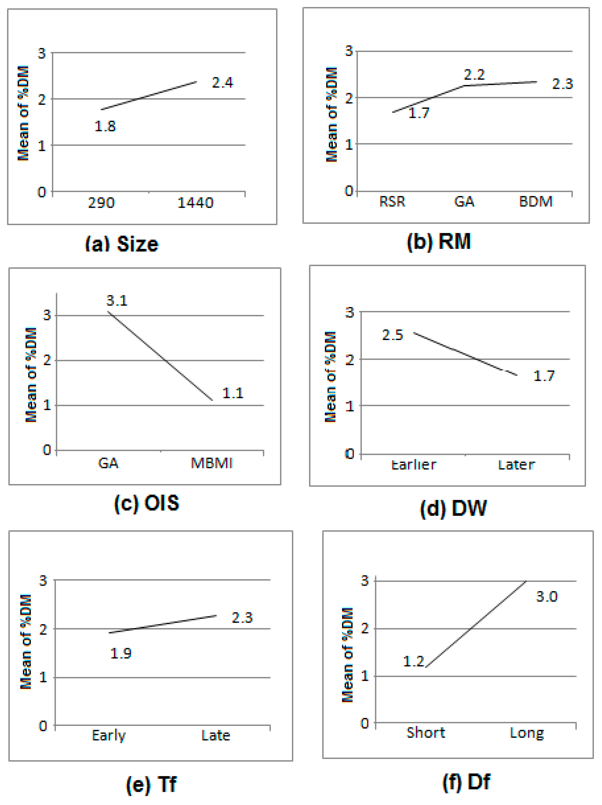
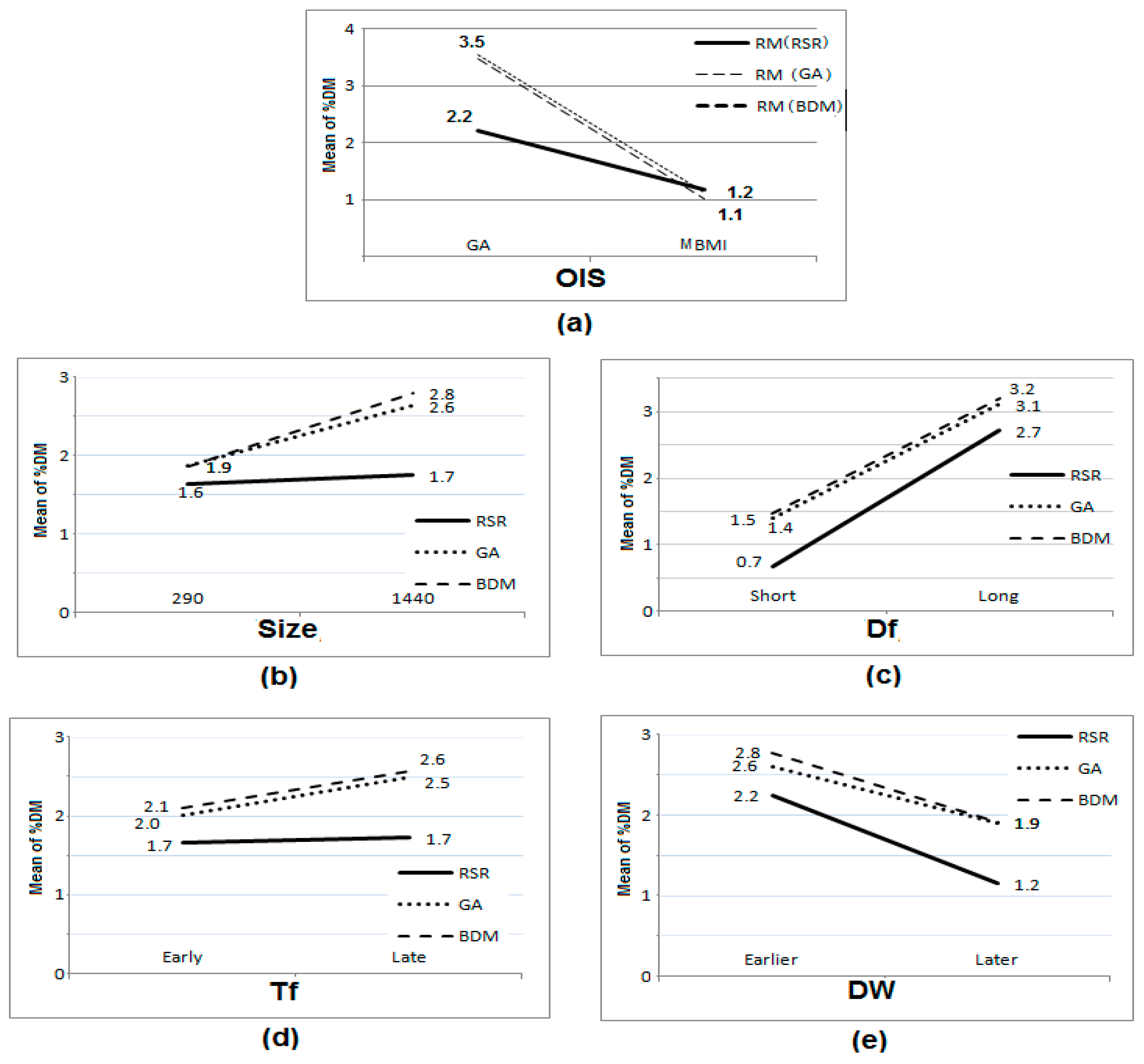
| Factors | Level 1 | Level 2 | Level 3 |
|---|---|---|---|
| F1: Size of the manufacturing system (size) | 290 | 1440 | For experimentation, the values are generated using random numbers for each replication independently. |
| F2: Extent of optimality of the initial schedule (OIS) | GA | MBMI | |
| F3: Number of disruptions occur and the workstations fail (DM) | Earlier | Later | |
| F4: Instant of disruption (Tf) | Early | Late | |
| F5: Failure duration (Df) | Short | Long | |
| F6: Rescheduling method (RM) | RSR | GA | BDM |
| Part No. | Processing Time of Operations on Workstations | ||||
|---|---|---|---|---|---|
| Machining Work Stations | Assembly Work Stations | ||||
| w1 | w2 | w3 | w4 | w5 | |
| j11 | O2 (12) | O3 (14) | O4 (9) | O9 (11) | O10 (16) |
| j12 | O5 (9) | O6 (14) | |||
| j13 | O7 (5) | O8 (12) | |||
| j21 | O11 (9) | O12 (7) | O13 (11) | O21 (15) | O22 (21) |
| j22 | O14 (9) | O15 (12) | |||
| j23 | O16 (11) | O17 (5) | |||
| j14 | O18 (10) | O19 (13) | O20 (4) | ||
| j31 | O23 (14) | O24 (5) | O25(9) | O30 (8) | O31 (15) |
| j32 | O26 (12) | O27 (13) | O28 (6) | ||
| j33 | O29 (12) | ||||
| Disruptions | Make-Span of the Original Schedule | Make-Span of Reschedule Using | ||||
|---|---|---|---|---|---|---|
| Failure Workstation Number | Instant of Failure | Duration of Failure | RSR | BDM | GA | |
| 2 | 20 | 15 | 125 | 135 | 133 | 133 |
| 2 | 40 | 5 | 130 | 126 | 126 | |
| 2 | 40 | 15 | 140 | 136 | 136 | |
| 3 | 20 | 15 | 138 | 130 | 130 | |
| 3 | 40 | 15 | 138 | 130 | 130 | |
| Name of Factors/Source of Variation | Sum of Squares | DOF | Mean Sum of Squares | FEst | FTab (95%) |
|---|---|---|---|---|---|
| Size | 26.26 | 1 | 26.26 | 11.23 | 3.84 |
| RM | 23.34 | 2 | 11.67 | 4.99 | 3.0 |
| OIS | 279.72 | 1 | 279.72 | 119.64 | 3.84 |
| DW | 55.36 | 1 | 55.36 | 23.68 | 3.84 |
| Tf | 8.42 | 1 | 8.42 | 3.60 | 3.84 |
| Df | 240.98 | 1 | 240.98 | 103.07 | 3.84 |
| OIS × RM | 30.55 | 3 | 10.18 | 4.36 | 2.6 |
| Size × RM | 8.94 | 3 | 2.98 | 1.27 | 2.6 |
| Df × RM | 1.54 | 3 | 0.51 | 0.22 | 2.6 |
| Tf × RM | 2.83 | 3 | 0.94 | 0.40 | 2.6 |
| DW × RM | 1.87 | 3 | 0.62 | 0.27 | 2.6 |
| Error | 633.58 | 271 | 2.34 |
Disclaimer/Publisher’s Note: The statements, opinions and data contained in all publications are solely those of the individual author(s) and contributor(s) and not of MDPI and/or the editor(s). MDPI and/or the editor(s) disclaim responsibility for any injury to people or property resulting from any ideas, methods, instructions or products referred to in the content. |
© 2023 by the authors. Licensee MDPI, Basel, Switzerland. This article is an open access article distributed under the terms and conditions of the Creative Commons Attribution (CC BY) license (https://creativecommons.org/licenses/by/4.0/).
Share and Cite
Bhongade, A.S.; Khodke, P.M.; Rehman, A.U.; Nikam, M.D.; Patil, P.D.; Suryavanshi, P. Managing Disruptions in a Flow-Shop Manufacturing System. Mathematics 2023, 11, 1731. https://doi.org/10.3390/math11071731
Bhongade AS, Khodke PM, Rehman AU, Nikam MD, Patil PD, Suryavanshi P. Managing Disruptions in a Flow-Shop Manufacturing System. Mathematics. 2023; 11(7):1731. https://doi.org/10.3390/math11071731
Chicago/Turabian StyleBhongade, Ajay Surendrarao, Prakash Manohar Khodke, Ateekh Ur Rehman, Manoj Dattatray Nikam, Prathamesh Dattatray Patil, and Pramod Suryavanshi. 2023. "Managing Disruptions in a Flow-Shop Manufacturing System" Mathematics 11, no. 7: 1731. https://doi.org/10.3390/math11071731
APA StyleBhongade, A. S., Khodke, P. M., Rehman, A. U., Nikam, M. D., Patil, P. D., & Suryavanshi, P. (2023). Managing Disruptions in a Flow-Shop Manufacturing System. Mathematics, 11(7), 1731. https://doi.org/10.3390/math11071731