Article

Exploring the Impact of Nonlinearities in Police Recruitment and Criminal Capture Rates: A Population Dynamics Approach

1
Department of Applied Mathematics, University of Johannesburg, Johannesburg 2006, South Africa
2
Department of Mathematical Sciences, University of Bath, Bath BA2 7AY, UK
*
Author to whom correspondence should be addressed.
Mathematics 2023, 11(7), 1669; https://doi.org/10.3390/math11071669
Submission received: 8 February 2023 / Revised: 20 March 2023 / Accepted: 28 March 2023 / Published: 30 March 2023
(This article belongs to the Special Issue Mathematical Population Dynamics and Epidemiology)

Abstract

:
The interplay between criminal activity and crime control/prevention measures is inherently dynamic. This paper presents a simple nonlinear dynamical system in which criminal activity levels are coupled to policing effort. Through the process of non-dimensionalisation and sensitivity analysis, policing efficiency and the responsiveness of policing effort are identified as key parameter groupings. An analysis of the system shows that bi-stability is a feature of the dynamics. When there is no feedback between criminal activity and police recruitment, a saddle-node bifurcation occurs and threshold levels of criminal activity are required for the activity to be maintained. When feedback is permitted, we also find a backward bifurcation and criminal activity can be contained for policing efficiency below its threshold level. We demonstrate proof of concept for how the model might be used as a predictive tool with real data.

1. Introduction

The growing interest in using mathematical modelling techniques to support qualitative and quantitative research in the Social Sciences means that dynamical systems previously applied in the life and health sciences are now being applied to a much broader range of contexts [1,2,3]. There are several roles that modelling can play but probably the most important is its predictive power. It allows the social scientist to explore how different assumptions will affect observations and, by linking model outcomes to available data, it may allow some assumptions to be discounted.
As a subset of the Social Sciences, the study of criminology has certainly benefited from the exploitation of the mathematical sciences [4,5,6,7]. Much of this work focuses on game theoretic models of individual choices and economic incentives [8,9,10,11] or on statistical methods to analyse complex spatio-temporal data sets [12,13,14]. Some work makes explicit reference to using mathematical models that are better known for exploring ecological or epidemiological concepts [15,16,17,18]. There is also a number of papers that use partial differential equations or other spatial modelling approaches [15,19,20,21], some of which explore the spread of criminal activity from hotspots [22,23].
To be effective, crime control strategies need to be relevant to the nature of the crime that they are meant to control—a police officer working on the street is unlikely to be effective against cybercrime. In this paper, we have chosen to explore the impact of policing on the control of criminal activity. The motivation for this rests on the debate around effective and efficient police recruitment strategies and how police recruitment should respond to changes in criminal activity [24].
As with the general crime models, previous mathematical models which explore the interaction between policing and criminal activity take a number of forms. There are time-dependent dynamical systems such as [25,26,27], spatio-temporal models [28] and algorithmic approaches [29,30]. Pertinent to our work, the model presented in [25] uses a nonlinear deterministic system to describe the interplay between criminal, non-criminal and police populations. The focus is on classic model analysis—steady states, numerical solutions, bifurcation and sensitivity. We also undertake these aspects of model analysis but extend ideas to identify physically relevant parameter groupings and to explain how the model could be used with data sets. In [18], the interaction between police and criminals is assumed to be competitive and a dynamical system is once again used to explore the interaction. However, outcomes on the scaling between police numbers and population size are compared with real data. There are also hybrid models such as [31], which discusses the interaction of criminals and the police in a three-population study and explores the issue of optimal behaviours.
The majority of this work (see [18]) is theoretical in nature and makes little attempt to integrate model results with data. In part, this may be due to the poor alignment of data with the model components. Previously, we addressed this issue [32] such that model formulation allows validation and parameterisation using the available data. That approach is used again here to create a model in which the variables are appropriate for comparison with data.
This paper is structured as follows. The model is presented in Section 2 and, through a steady-state analysis, key parameter groupings that drive model behaviour are extracted. Qualitative analysis of the model system is undertaken in Section 3 which identifies threshold behaviours. The analytical outcomes are applied to a small-scale data set of police numbers and criminal activity in Section 4. This is essentially a scoping exercise to demonstrate the potential of our model structure to contribute to understanding the interplay of criminal activity and crime prevention. Finally, the discussion in Section 5 highlights key findings and future avenues for exploration.

2. Mathematical Model

The model is built using the principle of Occam’s Razor [33] to describe the dynamic interaction between criminal activity C ( T ) and policing effort P ( T ) where T is the independent variable measuring time. It is constructed using the following assumptions:
  • The population size of the community which is subject to criminal activity is large. This allows us to assume that there are no population size constraints on the dynamical interaction between criminal activity and policing effort.
  • In the absence of any policing effort, the growth of criminal activity can be described by the logistic equation with intrinsic growth rate r and environmental carrying capacity K (which corresponds to the amount of criminal activity that could potentially occur in a given location);
  • Policing effort is analogous to a Holling type II [34] predation rate in which the amount of criminal activity stopped is described by a saturating function with maximum removal rate β and half-saturation constant Γ ;
  • In the absence of criminal activity, policing effort is maintained at a baseline level P b and, following any perturbation will return to that level at a rate σ ;
  • Policing effort may be influenced by the amount of criminal activity [24]. We represent that as a bounded positive influence f ( C ) such that 0 f ( C ) M for some positive constant M.
Combining these assumptions leads directly to the two-dimensional system of nonlinear differential equations:
d C ( t ) d T = r C 1 C K β C P Γ + C , d P ( t ) d T = σ [ P b P ] + f ( C ) ,
where all parameters are assumed to be positive.
To fully specify the problem, non-negative initial conditions C ( 0 ) > 0 , P ( 0 ) 0 are assumed. In this case, noting that
d C d T = 0 on C = 0 , d P d T = σ P b + f ( C ) > 0 on P = 0
it is apparent that solutions of the model system (1) remain in the positive quadrant for all time.
Moreover, our model solutions ( C ( t ) , P ( t ) ) remain bounded in the domain
Ω = ( C , P ) : 0 C K , 0 P P b + M σ
which can be demonstrated by noting that
d C d T 0 on C = K , and d P d T = f ( C ) M 0 on P = P b + M σ .
In the absence of P, the model obeys logistic growth and C approaches K as t and P P b in the absence of C as t .

2.1. Criminal Influence on Police Recruitment

Two distinct choices are made for f ( C ) :
Case 1: f ( C ) = 0 in which case the amount of criminal activity does not affect police recruitment rates;
Case 2: f ( C ) = λ C 1 + ϵ C where λ and ϵ are positive constants and the recruitment rate is a saturating function of the amount of criminal activity.

2.2. Non-Dimensionalisation

To determine key parameter groupings and to explore their impact on the observed dynamics the model system (1) is non-dimensionalised using the change of variables:
u = C K , v = P P b and t = r T ,
to obtain the rescaled system
d u d t = u [ 1 u ] Π 0 a u v a + u , d v d t = ϕ 1 v + b u c + u ,
with initial conditions u ( 0 ) = u 0 > 0 and v ( 0 ) = v 0 > 0 and dimensionless parameters
Π 0 = β P b r Γ , a = Γ K , b = λ ϵ σ P b , c = 1 ϵ K ϕ = σ r .
The dimensionless parameters are defined as follows:
  • Π 0 measures the amount of criminal activity stopped per unit policing effort over the time it takes to initiate new criminal activity when policing effort is most responsive to the amount of criminal activity (i.e., when u is small). This is labelled policing efficiency;
  • a measures how quickly policing effort responds to increases in criminal activity such that small values of a correspond to a more rapid response.This is labelled responsiveness of policing effort. Since the domain is restricted to 0 u 1 , when a > 1 nonlinearity of the effect of policing effort on reducing criminal activity will NOT be observed in the dynamics. This is entirely feasible because it means that policing effectiveness is broadly proportional to the amount of criminal activity in the region. This feature is useful to recall below in Section 3 when we come to observe structural differences in the system depending on whether a is less than or greater than 1. For completeness, note that if a < 1 , nonlinearity in policing control will be observed in the dynamical system. This corresponds to the case where increases in criminal activity cannot be matched by policing control;
  • b measures the increase in policing effort per criminal activity relative to the baseline over the average time associated with police recruitment and turnover rates. Indirect feedback of criminal activity on that activity due to the criminal-policing interaction. This is labelled criminal-induced policing impact;
  • c measures the effect or influence of the carrying capacity of criminal activity on the growth of policing effort.
These definitions provide useful insight into the important components of the model system; they are exploited in the following section where we consider the stability of the steady-state solutions and explore the associated bifurcation structure.
Since both C and P are bounded (2), it follows that u and v are also bounded variables.

3. Model Analysis

Model exploration is focused around a steady state analysis which reveals interesting bifurcation behaviour and identifies bistability properties of the model system. Linear stability analysis is used to show the existence of saddle-node bifurcation points and when f ( C ) 0 , backward bifrucation behaviour is also identified. Before embarking on that endeavour, a sensitivity analysis is undertaken to identify the significance of each parameter on the model solution.

3.1. Sensitivity Analysis

We apply a robust sensitivity test to determine the relationship between the parameter groups and our model solutions, focusing particularly on the impact of parameters on policing effort, v * . The Latin Hypercube Sampling (LHS) method is used to create sample points [35]. These sample points are used within a Partial Rank Correlation Coefficient (PRCC) technique [35,36], alongside a testing parameter group. The parameters in the testing group were chosen arbitrarily to be a = 0.1962 , b = 0.6 , c = 0.1 , Π 0 = 0.9419 and ϕ = 0.7043 ; the results obtained, which are shown in Figure 1a,b, are consistent with alternative testing group parameter choices.
Based on these results, bifurcation analysis was focused on the two parameters a and Π 0 to explore the range of model behaviours. In principle, it appears that a Hopf bifurcation may be possible for this system in the case where f ( C ) 0 . Extensive numerical exploration has failed to identify limit cycle solutions in this case and so we may postulate that these solutions are not stable if they exist. We do not explore this phenomenon further here, but may revisit these dynamics in future publications. At the end of this section, we also comment on the impact of the other dimensionless parameters ϕ , b and c.

3.2. Steady State Analysis

To simplify algebraic calculations, the model system (3) is rewritten in the form:
d u d t = η ( u ) g ( u ) v , d v d t = ϕ ( 1 v ) + f ( u ) ,
where
η ( u ) = Π 0 a u a + u g ( u ) = ( 1 u ) ( a + u ) Π 0 a ,
and f ( u ) = 0 or f ( u ) = b u c + u .
For both choices of f ( u ) the semi-trivial steady state ( u * , v * ) = ( 0 , 1 ) exists whilst any non-trivial steady states are real solutions of
g ( u * ) = 1 + f ( u * ) , v * = g ( u * ) ,
which satisfy 0 u * 1 .
The local stability of a steady state ( u * , v * ) is determined using the Jacobian matrix
J ( u * , v * ) = η ( u * ) [ g ( u * ) v * ] + η ( u * ) g ( u * ) η ( u * ) ϕ f ( u * ) ϕ ,
by evaluating the trace and determinant (details to follow for the specific cases).
Below we consider the semi-trivial and coexistence steady states separately. In each case, stability conditions are determined and the results are presented in bifurcation diagrams.
Case 1: Semi-trivial steady state
The Jacobian matrix (5) becomes
J E 0 ( u * , v * ) = η ( 0 ) 1 Π 0 1 0 ϕ f ( 0 ) ϕ
from which we can deduce that the steady state is a locally stable node if Π 0 > 1 and an unstable saddle point if Π 0 < 1 . This is true for both choices of f ( u ) .
Case 2: Non-trivial steady states
For all non-trivial steady states, the Trace and Determinant of (5) are
Tr ( J ) = η ( u * ) g ( u * ) ϕ , Det ( J ) = ϕ f ( u * ) η ( u * ) ϕ η ( u * ) g ( u * ) .
Case 2a: No criminal influence on police recruitment, f ( u ) = 0
With f ( u ) = 0 , (4) simplifies to the quadratic equation for u *
u * 2 + ( a 1 ) u * + ( Π 0 1 ) a = 0
solutions of which are given as
u + / * = ( 1 a ) ± ( 1 a ) 2 4 a ( Π 0 1 ) 2 .
By observation of (7) we note that
  • Solutions of (7) will only be real if ( 1 a ) 2 > 4 a ( Π 0 1 ) (note that this is always satisfied if Π 0 < 1 );
  • If Π 0 < 1 , there is a single positive steady state solution (the other solution is negative);
  • If Π 0 > 1 , then there will be two positive solutions provided that a < 1 and no positive solutions if a > 1 .
We also observe that, when f ( C ) = 0 , the eigenvalues of the Jacobian matrix (5) are real, given as
λ 1 = η ( u * ) g ( u * ) , λ 2 = ϕ .
Therefore, a non-trivial steady state is a locally stable node provided g ( u * ) < 0 , and an unstable saddle if g ( u * ) < 0 . Now
g ( u * ) = ( 1 a ) 2 u * Π 0 a
and so, by substitution, we deduce that whenever the steady states exist, u * is an unstable saddle point and u + * is a stable node.
In summary:
  • For 0 < a < 1 :
    There is a single non-trivial stable steady state if Π 0 < 1 ;
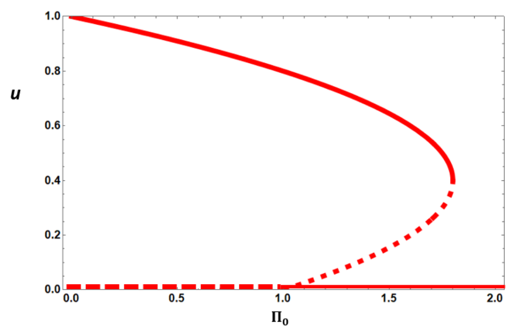
    For 1 < Π 0 < ( 1 + a ) 2 4 a there are two non-trivial steady states the smaller of which is unstable and the larger of which is locally stable;
    For Π 0 > ( 1 + a ) 2 4 a , there is no non-trivial steady state.
These results are presented using a bifurcation diagram shown in Figure 2.
  • For a > 1 , the following results are obtained:
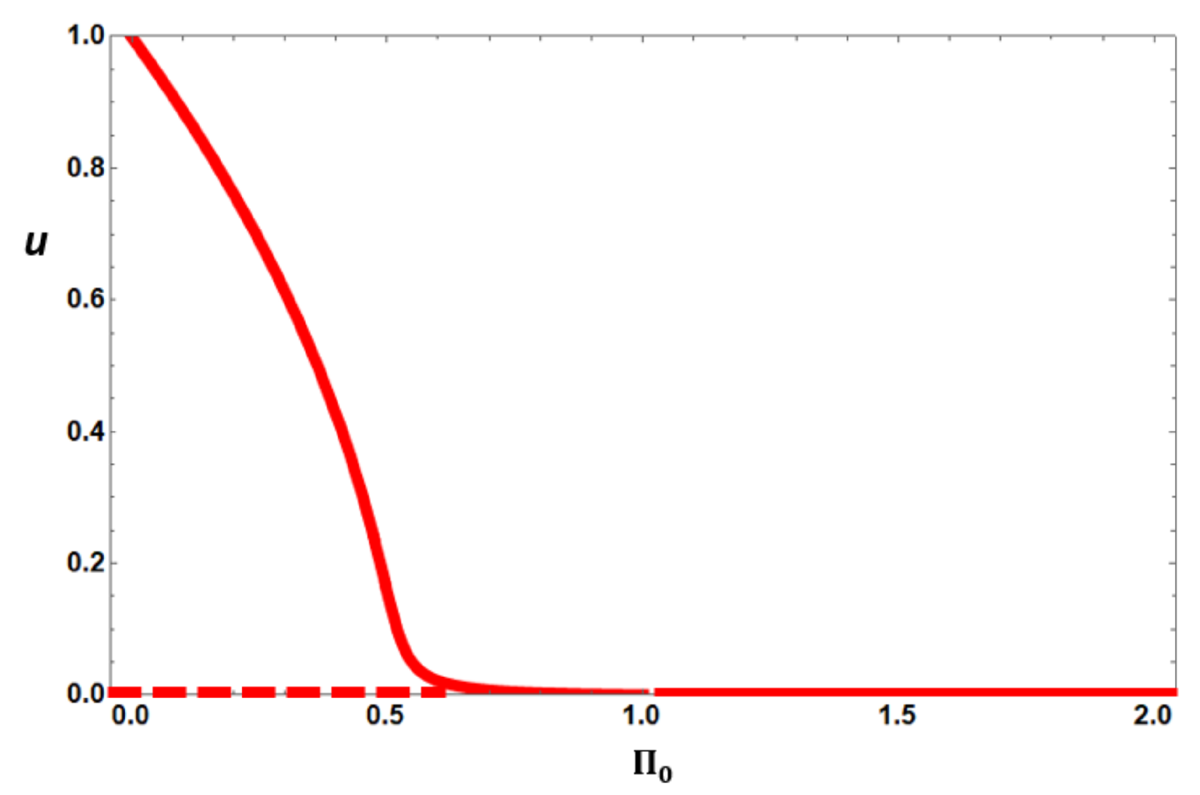
    For Π 0 < 1 there is a single stable non-trivial steady state.
    For Π 0 > 1 there is no non-trivial steady state.
These results are summarised graphically through the bifurcation diagram in Figure 3.
Comparing Figure 2 with Figure 3 we notice that the high responsiveness of policing effort to criminal activity ( a > 1 ) results in a one-to-one relationship between criminal activity levels and policing efficiency such that, once the efficiency exceeds threshold levels ( Π 0 = 1 ), the criminal activity could be eradicated theoretically. By contrast, if there is a low responsiveness ( a < 1 ), even when that threshold is exceeded, criminal activity can be maintained if u ( 0 ) > u * , i.e., if the initial criminal activity level is sufficiently great.
Case 2b: Criminal influence on police recruitment, f ( u ) > 0
This case is more complex due to the positive feedback between criminal activity and policing effort. When solving (4), the cubic equation
μ 1 ( u * ) 3 + μ 2 ( u * ) 2 + μ 3 u * + μ 4 = 0
is obtained where
μ 1 = 1 , μ 2 = a + c 1 , μ 3 = Π 0 a ( 1 + b ) a + a c c and μ 4 = a c ( Π 0 1 ) .
Preliminary analysis using Descartes’s Rule of Signs identifies parameter constraints associated with the maximum number of positive steady state solutions in this case. See Table 1.
The information provided in Table 1 leads to the following observations:
  • For a < 1 :
    For Π 0 > 1 there is no positive nontrivial steady state if a + c > 1 whilst there are two nontrivial positive steady states if a + c < 1 .
    For Π 0 < 1 there is a single positive nontrivial steady state if
    b c < 1 Π 0 1 a 1 + ( 1 Π 0 ) c
    and there will be three positive nontrivial steady states if
    c + a < 1 and b c > 1 Π 0 1 a 1 + ( 1 Π 0 ) c .
    It is worth noting that this final condition giving rise to three positive nontrivial steady states is once again a condition on police responsiveness a falling below a threshold (which in this case is 1 c ).
    These results are shown graphically through the bifurcation diagram in Figure 4. We also show, in Figure 5, a phase-line diagram and solution trajectories in the parameter space where bistability is observed with three non-trivial steady state solutions.
  • For a > 1 :
    When Π 0 > 1 there is no positive nontrivial steady state;
    When Π 0 < 1 there is a single positive nontrivial steady state.
These results are summarised graphically through the bifurcation diagram in Figure 6.

Other Observations

These observations are made assuming that other parameters remain fixed.
  • Increasing the value of ϕ (the ratio of baseline rates of increase in policing effort to criminal activity) reduces the potential to exhibit oscillatory dynamics as the steady state changes from a stable focus to a stable node.
  • Increasing b (criminal-induced policing effort) increases the amplitude of the transient oscillatory dynamics by increasing the value of the determinant of the Jacobian which affects the size of this oscillation.
  • Increasing c (corresponding to a reduction in the size of the environmental carrying capacity for criminal activity) reduces the number of non-trivial steady states that would be observed in the system. In relation to the model structures, the increase lowers the threshold for police responsiveness ( a < 1 c ) which produces the bistable behaviours that we observe.
In principle, with f ( C ) > 0 , the system may admit limit cycle solutions, which would arise from a Hopf bifurcation. Although we are able to write down conditions for this, we were unable to identify any stable limit cycles in our system. Further study, which may benefit from techniques of numerical continuation bifurcation analysis [37], could be appropriate.

4. Linking the Model to Data

There are a number of challenges associated with using the model and its predictions alongside data. One of the more significant of these is linking police-reported crimes with the impact it has on whether and/or for how long, it results in a criminal no longer engaging in criminal activity within the locality of the crime for which they have been arrested by the police. We will explore that dynamic in future work. For now we assume that the reduction in criminal activity is directly proportional to the number of reported criminal incidents, an observation that we found to have some credibility in previous work [32].
It is also important to consider the nature of the crime. We chose to restrict ourselves to crimes where frontline police attend the scene of the crime but we did not distinguish the nature of the crime. This was motivated by the data which we used where frontline police numbers are available together with crime locations and incident numbers.
We arbitrarily used data from the Avon and Somerset Constabulary (because it includes the City of Bath where one of the authors is based). Although data on police numbers is readily available since 2010, changes in crime reporting mean that we only have crime incident data since 2020, spanning 3 calendar years. Notwithstanding this limitation, we found that we were able to use the data in conjunction with the model to give interesting observations. The data, presented in Table 2, includes the number of frontline police in the years 2013–2019 to note that whilst the numbers show some fluctuation, they have been maintained in the range 2275–2620 for the past decade.
From the table, the first observation that can be made is to notice that the number of crimes per police per year has remained essentially constant over the past 3 years. This suggests that levels of policing effort are proportional to criminal activity so this data corresponds to the case where f ( C ) > 0 .
Next, we observe that both the policing and crime levels are increasing over time which positions the data within the region of phase space where both v < g ( u ) and v < 1 + f ( u ) . As can be seen in Figure 5, if the dynamics are such that a containment steady state exists ( u * small, v * > 1 ), it is possible, without any change in recruitment strategy, that criminal activity may be contained. However, that is not guaranteed, and even with a slight perturbation from conditions that support containment, the outcome may be outbreak levels of criminal activity. If there is concern that criminal activity levels might not be contained, then one strategy which could be implemented is to increase the responsiveness to policing such that a > 1 and the dynamics are as shown in Figure 6. This would give some certainty to the predictions because they would no longer be dependent on the current state of the system, simply the policing efficiency threshold ( Π 0 = 1 ).

5. Discussion

In this paper, we have explored the dynamic consequences of criminal activity being constrained by policing effort under two distinct models of police recruitment. The model form includes a physically realistic upper bound on the amount of criminal activity that can be stopped per unit time per unit policing effort. This is important because the presence or absence of the saturation effect from this term produces qualitatively different dynamical behaviours (comparing Figure 2 and Figure 3 or Figure 4 and Figure 5). Put another way, we have identified threshold behaviour at a = 1 (or in dimensional terms when Γ = K ). Using this in a predictive context, if estimates of the local carrying capacity for criminal activity can be found, control strategies could be focused around interventions that would change the model parameter Γ .
The other important model construct that we have focused our analysis around is whether or not criminal activity levels impact police recruitment. This consideration was one of the key motivations behind our study, and therefore, we were excited to observe qualitatively different outcomes under the two conditions. In particular, the backward bifurcation which occurs when the positive feedback between criminal activity and police recruitment is included is not observed when that feedback is absent.
The process of non-dimensionalisation has been hugely beneficial. This is not surprising for an applied mathematician but it is important to emphasise here as we contribute to the relatively new field of deterministic modelling for criminology. We were able to systematically use the dimensionless parameter groupings to interpret results physically.
Of course, this work hugely simplifies the highly complex dynamical system that it purports to describe, which means that any results presented must be cautiously interpreted, always referring back to the underlying model assumptions [40]. Using a continuous time dynamical system without delays suggests that where feedback occurs, it does so instantly. This is unlikely to be the case, particularly for police recruitment processes. In future work, we may consider how metered recruitment alters the dynamics (essentially replacing f ( C ) with an integral that measures cumulative criminal activity over some period of time). We also acknowledge that the loss of criminal activity due to policing effort uses a function often found in predator–prey models [41] and again is instantaneous. This term would benefit from further consideration to determine how realistic it is in relation to the process of police control and arraignment.
As we described in the Introduction, the use of dynamical systems theory is starting to establish itself as a useful tool in the toolkit for understanding interactions between criminal activity and its control. Continuing the approach that we have taken previously [32], we have shown how the model may be used alongside data as a predictive tool. Additional data would be needed to be confident about any predictions, but we have shown, once again, proof of concept. In this way, the modelling exercise presented here makes a valuable, and distinctive, contribution to the growing literature of deterministic modelling in criminology [1,2].

Author Contributions

Conceptualization, F.N.; Methodology, K.A.J.W.; Validation, F.N.; Formal analysis, T.C. and K.A.J.W.; Investigation, T.C.; Resources, F.N.; Writing—original draft, T.C.; Writing—review & editing, F.N. and K.A.J.W.; Supervision, F.N. All authors have read and agreed to the published version of the manuscript.

Funding

This research received no external funding.

Data Availability Statement

The Matlab and Mathematica codes used to generate figures presented in the paper are avaiable from the corresponding author upon request.

Acknowledgments

The authors authors acknowledge the support of their respective institutions in the production of the manuscript. The authors also acknowledge that this paper is part of the doctoral research work of T.C.

Conflicts of Interest

The authors declare that there is no conflict of interest regarding the publication of this paper.

References

  1. Saaty, T.L.; Alexander, J.M. Thinking with Models: Mathematical Models in the Physical, Biological, and Social Sciences; RWS Publications: Pittsburgh, PA, USA, 1981; Volume 2. [Google Scholar]
  2. Zimmermann, H.J. Testability and meaning of mathematical models in social sciences. Math. Model. 1980, 1, 123–139. [Google Scholar] [CrossRef] [Green Version]
  3. Weidlich, W. Sociodynamics: A Systematic Approach to Mathematical Modelling in the Social Sciences; Courier Corporation: North Chelmsford, MA, USA, 2006. [Google Scholar]
  4. Bertozzi, A. Mathematics of Crime—Mathematical Modelling of Complex Systems; University of Oxford: Oxford, UK, 2016; p. 4. [Google Scholar]
  5. Sooknanan, J.; Bhatt, B.; Comissiong, D. Catching a gang—A matematical model of the spread of gangs in a population treated as an infectious disease. Int. J. Pure Appl. Math. 2013, 83, 25–43. [Google Scholar] [CrossRef] [Green Version]
  6. Bertozzi, A.; Johnson, S.; Ward, M. Mathematical modelling of crime and security. Eur. J. Appl. Math. 2016, 27, 311–316. [Google Scholar] [CrossRef] [Green Version]
  7. Primicerio, M. The role of mathematical modelling in modern criminology Comment on “Statistical physics of crime: A review” by MR D’Orsogna and M. Perc. Phys. Life Rev. 2015, 12, 34–35. [Google Scholar] [CrossRef] [PubMed]
  8. Wu, C.K.; Chen, Y.M.; Wu, D.; Chi, C.L. A game theory approach for assessment of risk and deployment of police patrols in response to criminal activity in San Francisco. Risk Anal. 2020, 40, 534–549. [Google Scholar] [CrossRef]
  9. Zhang, C.; Gholami, S.; Kar, D.; Sinha, A.; Jain, M.; Goyal, R.; Tambe, M. Keeping pace with criminals: An extended study of designing patrol allocation against adaptive opportunistic criminals. Games 2016, 7, 15. [Google Scholar] [CrossRef] [Green Version]
  10. Short, M.; Brantingham, P.; D’Orsogna, M. Cooperation and punishment in an adversarial game: How defectors pave the way to a peaceful society. Phys. Rev. E 2010, 82, 66–114. [Google Scholar] [CrossRef] [Green Version]
  11. De Mesquita, B.B.; Cohen, L.E. Self-interest, equity and crime control—A game-theoretic analysis of criminal decision making. Criminology 1995, 33, 483–518. [Google Scholar] [CrossRef]
  12. Short, M.; D’Orsogna, M.; Pasour, V.; Tita, G.; Brabtingham, P.; Bertozzi, A.; Chayes, L. A statistical model of criminal behaviour. Math. Model. Methods Appl. Sci. 2008, 18, 1249–1267. [Google Scholar] [CrossRef]
  13. Baloian, N.; Bassaletti, C.E.; Fernández, M.; Figueroa, O.; Fuentes, P.; Manasevich, R.; Orchard, M.; Peñafiel, S.; Pino, J.A.; Vergara, M. Crime prediction using patterns and context. In Proceedings of the 2017 IEEE 21st International Conference on Computer Supported Cooperative Work in Design (CSCWD), Wellington, New Zealand, 26–28 April 2017; pp. 2–9. [Google Scholar]
  14. Wang, D.; Ding, W.; Lo, H.; Morabito, M.; Chen, P.; Salazar, J.; Stepinski, T. Understanding the spatial distribution of crime based on its related variables using geospatial discriminative patterns. Comput. Environ. Urban Syst. 2013, 39, 93–106. [Google Scholar] [CrossRef]
  15. Manasevich, R.; Phan, Q.H.; Souplet, P. Global existence of solutions for a chemotaxis-type system arising in crime modelling. Eur. J. Appl. Math. 2013, 24, 273–296. [Google Scholar] [CrossRef]
  16. González-Parra, G.; Chen-Charpentier, B.; Kojouharov, H.V. Mathematical modeling of crime as a social epidemic. J. Interdiscip. Math. 2018, 21, 623–643. [Google Scholar] [CrossRef]
  17. Perc, M.; Donnay, K.; Helbing, D. Understanding recurrent crime as system-immanent collective behavior. PLoS ONE 2013, 8, e76063. [Google Scholar] [CrossRef] [PubMed] [Green Version]
  18. Banerjee, S.; Van Hentenryck, P.; Cebrian, M. Competitive dynamics between criminals and law enforcement explains the super-linear scaling of crime in cities. Palgrave Commun. 2015, 1, 15022. [Google Scholar] [CrossRef] [Green Version]
  19. Brantingham, P.J.; Tita, G. Offender mobility and crime pattern formation from first principles. In Artificial Crime Analysis Systems: Using Computer Simulations and Geographic Information Systems; IGI Global: Hershey, PA, USA, 2008; pp. 193–208. [Google Scholar]
  20. Cracolici, M.F.; Uberti, T.E. Geographical distribution of crime in Italian provinces: A spatial econometric analysis. Jahrb. Reg. 2009, 29, 1–28. [Google Scholar] [CrossRef] [Green Version]
  21. Brown, M.A. Modelling the spatial distribution of suburban crime. Econ. Geogr. 1982, 58, 247–261. [Google Scholar] [CrossRef]
  22. Short, M.B.; Bertozzi, A.L.; Brantingham, P.J. Nonlinear patterns in urban crime: Hotspots, bifurcations, and suppression. SIAM J. Appl. Dyn. Syst. 2010, 9, 462–483. [Google Scholar] [CrossRef] [Green Version]
  23. Lloyd, D.J.; O’Farrell, H. On localised hotspots of an urban crime model. Phys. D Nonlinear Phenom. 2013, 253, 23–39. [Google Scholar] [CrossRef]
  24. McCabe, J. An Analysis of Police Department Staffing: How Many Officers do You Really Need? 2019. Available online: https://icma.org/sites/default/files/305747_Analysis%20of%20Police%20Department%20Staffing%20_%20McCabe.pdf (accessed on 27 July 2021).
  25. Misra, A. Modeling the effect of police deterrence on the prevalence of crime in the society. Appl. Math. Comput. 2014, 237, 531–545. [Google Scholar] [CrossRef]
  26. Lacey, A.; Tsardakas, M. A mathematical model of serious and minor criminal activity. Eur. J. Appl. Math. 2016, 27, 403–421. [Google Scholar] [CrossRef] [Green Version]
  27. Pitcher, A.B. Adding police to a mathematical model of burglary. Eur. J. Appl. Math. 2010, 21, 401–419. [Google Scholar] [CrossRef]
  28. Short, M.B.; Brantingham, P.J.; Bertozzi, A.L.; Tita, G.E. Dissipation and displacement of hotspots in reaction-diffusion models of crime. Proc. Natl. Acad. Sci. USA 2010, 107, 3961–3965. [Google Scholar] [CrossRef] [Green Version]
  29. Moses, L.B.; Chan, J. Algorithmic prediction in policing: Assumptions, evaluation, and accountability. Polic. Soc. 2018, 28, 806–822. [Google Scholar] [CrossRef] [Green Version]
  30. Jones, P.A.; Brantingham, J.; Chayes, L.R. Statistical models of criminal behaviour: The effects of law enforcement actions. Math. Model. Methods Appl. Sci. 2010, 20, 1397–1423. [Google Scholar] [CrossRef] [Green Version]
  31. Coclite, G.M.; Garavello, M.; Spinolo, L. A mathematical model for piracy control through police response. Nonlinear Differ. Equ. Appl. 2017, 24, 48. [Google Scholar] [CrossRef]
  32. Jane White, K.; Campillo-Funollet, E.; Nyabadza, F.; Cusseddu, D.; Kasumo, C.; Imbusi, N.M.; Juma, V.O.; Meir, A.; Marijani, T. Towards understanding crime dynamics in a heterogeneous environment: A mathematical approach. J. Interdiscip. Math. 2021, 24, 2139–2159. [Google Scholar] [CrossRef]
  33. Walsh, D. Occam’s Razor: A Principle of Intellectual Elegance. Am. Philos. Q. 1979, 16, 241–244. [Google Scholar]
  34. Holling, C.S. Some characteristics of simple types of predation and parasitism. Can. Entomol. 1959, 91, 385–398. [Google Scholar] [CrossRef]
  35. Boloye, G. Latin Hypercube Sampling and Partial Rank Correlation Coefficient Analysis Applied to an Optimal Control Problem. Available online: https://trace.tennessee.edu/utk_gradthes/1278 (accessed on 20 August 2022).
  36. Wu, J.; Dhingra, R.; Gambhir, M.; Remais, J.V. Sensitivity analysis of infectious disease models: Methods, advances and their application. J. R. Soc. Interface 2013, 10, 20121018. [Google Scholar] [CrossRef] [PubMed] [Green Version]
  37. Khanghahi, M.J.; Ghaziani, R.K. Bifurcation Analysis of a Modified May–Holling–Tanner Predator–Prey Model with Allee Effect. Bull. Iran. Math. Soc. 2022, 48, 3405–3437. [Google Scholar] [CrossRef]
  38. Official Statistics Police Officer Uplift, England and Wales, Quarterly Update to 31 March 2022. Available online: https://www.gov.uk/government/statistics/police-officer-uplift-quarterly-update-to-march-2022/police-officer-uplift-england-and-wales-quarterly-update-to-31-march-2022 (accessed on 27 August 2022).
  39. Data Downloads. Available online: https://data.police.uk/data/ (accessed on 27 August 2022).
  40. Roberts, M.; Andreasen, V.L.A.; Pellis, L. Nine challenges for deterministic epidemic models. Epidemics 2015, 10, 49–53. [Google Scholar] [CrossRef] [PubMed] [Green Version]
  41. Tewa, J.; Djeumen, V.; Bowong, S. Predator–Prey model with Holling response function of type II and SIS infectious disease. Appl. Math. Model. 2012, 37, 4825–4841. [Google Scholar] [CrossRef]
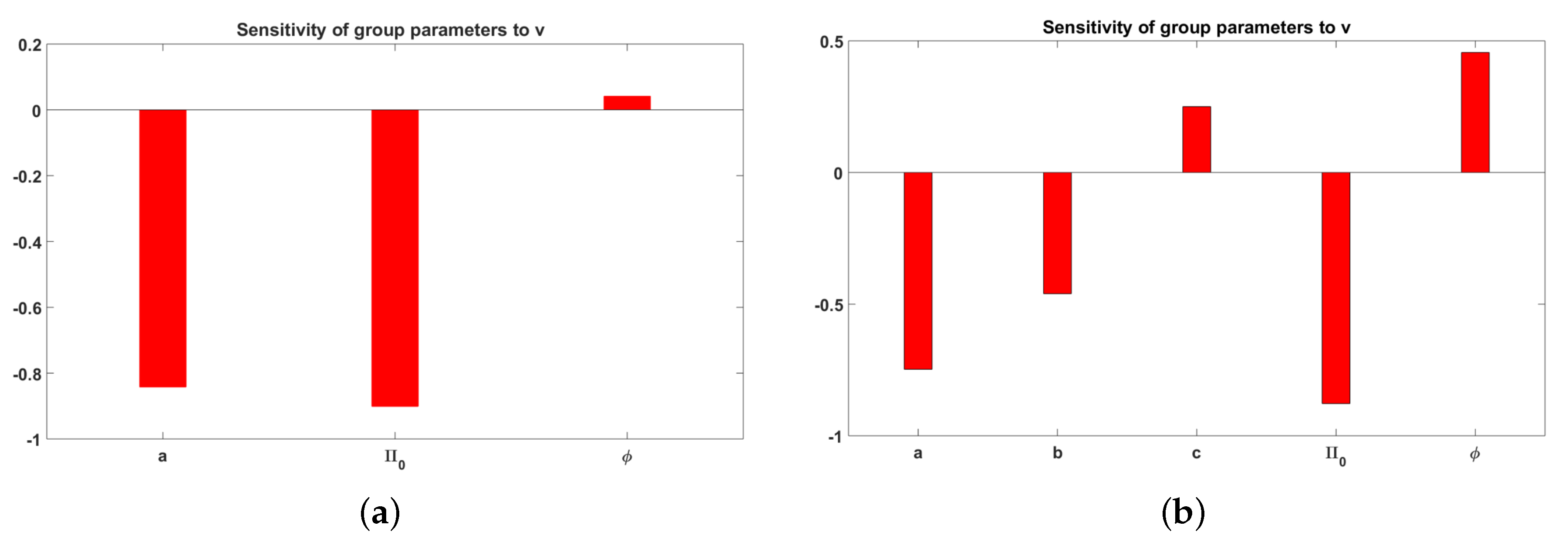
Figure 1. A depiction of the sensitivity of the non-trivial steady state v to changes in model parameters. Baseline parameters were chosen arbitrarily to take values a = 0.1962 , Π 0 = 0.9419 , ϕ = 0.7043 , b = 0.6 , c = 0.1 and the dimensionless time t = 280 was arbitrarily chosen to ensure that in all cases the steady state had been reached. (a) Case 1: f ( C ) = 0 . (b) Case 2: f ( C ) > 0 .
Mathematics 11 01669 g001
Figure 2. A bifurcation diagram linking steady state criminal activity levels to policing efficiency. The solid line corresponds to a stable steady state and the dashed line to an unstable steady state. In this case, with a = 0.2 , we are considering low policing responsiveness to criminal activity. A saddle-node bifurcation is observed.
Mathematics 11 01669 g002
Figure 3. A bifurcation diagram linking steady state criminal activity levels to policing efficiency. The solid line corresponds to a stable steady state and the dashed line to an unstable steady state. In this case, with a = 1.2 , we are considering high policing responsiveness to criminal activity. A transcritical bifurcation is observed.
Mathematics 11 01669 g003
Figure 4. A bifurcation diagram linking steady state criminal activity levels to policing efficiency when police recruitment is linked to criminal activity. Solid lines correspond to stable steady states and dashed lines to unstable steady states. The parameters used to create these figures were a = 0.2 , b = 1.6 and c = 0.06 which means that the system represents the scenario of low policing responsiveness to criminal activity. Moreover, since a + c < 1 , the bistable dynamics predicted in Table 1 are observed. In (a), the full bifurcation diagram is presented; in (b), we have zoomed in around the backward bifurcation.
Mathematics 11 01669 g004
Figure 5. A phase plane and time profiles for u ( t ) and v ( t ) in parameter space which gives rise to the bifurcation diagram shown in Figure 4. In this case, we use parameter values Π 0 = 0.7 , a = 0.2 , ϕ = 1 , b = 1.6 and c = 0.06 . In (a), the black solid curve corresponds to the v-nullcline and the black dashed curve to the u-nullcline. The other two coloured curves show solution trajectories in the phase plane. In (b), time-dependent solution trajectories are shown and these highlight the bistable nature of the dynamics (using initial conditions that are close together in phase space).
Mathematics 11 01669 g005
Figure 6. A bifurcation diagram linking steady state criminal activity levels to policing efficiency. The solid line corresponds to a stable steady state and the dashed line to an unstable steady state. In this case, with a = 1.2 , b = 0.963 and c = 0.01 , the system represents high policing responsiveness to criminal activity. A transcritical bifurcation is observed.
Mathematics 11 01669 g006
Table 1. Sign of polynomial coefficients which can be used with Descartes’s rule of signs to determine the number of positive steady states of the model system.
Condition μ 1 μ 2 μ 3 μ 4 Max # +ve st.st.
a > 1 , Π 0 > 1 ++++Zero
a > 1 , Π 0 < 1 +++ ( c + a > 1 )One
++− ( c + a < 1 )One
a < 1 , Π 0 > 1 +− ( c + a < 1 )++Two
++ ( c + a > 1 )++Zero
a < 1 , Π 0 < 1 +− ( c + a < 1 )+ ( b > c Π 0 1 a 1 + 1 Π 0 c )Three
+Either +/−− ( b < c Π 0 1 a 1 + 1 Π 0 c )One
Table 2. Data since 2010 on number of frontline police in Avon and Somerset together with the number of crimes reported for the 3 years 2020–2022 inclusive. Police numbers were obtained from the annual reporting tool for the UK government [38] and crimes with police incident numbers by the local police force [38,39].
YearFrontline Police NumbersNumber Crimes ReportedNumber Crimes per Police per Year
20132565N/AN/A
20142394N/AN/A
20152449N/AN/A
20162475N/AN/A
20172449N/AN/A
20182319N/AN/A
20192277N/AN/A
20202380128,86054
20212498132,45553
20222611140,61954
Disclaimer/Publisher’s Note: The statements, opinions and data contained in all publications are solely those of the individual author(s) and contributor(s) and not of MDPI and/or the editor(s). MDPI and/or the editor(s) disclaim responsibility for any injury to people or property resulting from any ideas, methods, instructions or products referred to in the content.