An Adaptive Multiple-Asset Portfolio Strategy with User-Specified Risk Tolerance

Abstract

We improve the traditional simple moving average strategy by incorporating an investor-specific risk tolerance into the method. We then propose a multiasset generalized moving average crossover (MGMA) strategy. The MGMA strategies allocate wealth between risky assets and risk-free assets in an adaptive manner, with the risk tolerance specified by an investor. We derive the expected log-utility of wealth, which allows us to estimate the optimal allocation parameters. The algorithm using our MGMA strategy is also presented. As the multiple risky assets can have different variability levels and could have various degrees of correlations, this trading strategy is evaluated on both simulated data and global high-frequency exchange-traded fund (ETF) data. It is shown that the MGMA strategies could significantly increase both the investor’s expected utility of wealth and the investor’s expected wealth.

1. Introduction

This paper provides an optimal and adaptive portfolio allocation strategy based on the technical analysis of a diversified investment portfolio. The investment portfolio often contains more than one risky asset to avert possible significant loss. Portfolio allocation is an important strategy for investors and traders, and they are interested in an optimal allocation when they have enough capital to invest in more than two assets. They might want to allocate the wealth not only between one risk-free asset and another risky asset but also among different risky assets. The common approach is to assign equal weights when allocating the wealth among the risky assets, which, however, is not always optimal. We believe that an allocation amount should be a function of the investor’s specified risk tolerance, and this consideration could lead to a more favorable investment outcome. We focus on finding optimal trading strategies based on technical analysis, such as moving averages for building a multiple-asset portfolio. We propose a multiasset generalized moving average crossover (MGMA) strategy. This strategy can allocate wealth not only between one risky asset and another risk-free asset but also among different risky assets, with the risk tolerance specified by the investor. It can also increase both the investor’s expected utility of wealth and the investor’s expected wealth.

Technical analysis is widely adopted by investors in practice. The empirical evidence, including the predicted performance of a stock return, demonstrates the usefulness of technical analysis (see [1,2,3,4]). Among all the technical analysis methods, the moving average strategy is the simplest and most popular trading rule. Ref. [1] appeared to be the first article to provide strong evidence of profitability by using a moving average technique in analyzing daily Dow Jones Industrial Average (DJIA) data. The moving average strategy in technical analysis follows an all-or-nothing investment strategy: when a buy signal is triggered by the moving average crossover (MA) strategy, the investor should allocate all of his/her wealth to the stocks of interest; when a sell signal is triggered by MA, the investor should allocate none of the wealth into the stocks by selling all the current holdings. Thus, this simple moving average strategy suffers from a well-known drawback, since its allocation is always either 100% or 0%. Ref. [2] provided further evidence based on different time series data obtained from financial markets. These studies have generated further research interest on moving average strategies. However, most of the studies have been focused on validating the strategy using different data sets. The conclusions are mixed and inconclusive (see [5,6,7,8,9]). An increasing number of studies are focused on the predictive power of a moving average technique (see [10,11,12,13,14,15]). Ref. [16] provided the first theoretical analysis for this simple moving average crossover strategy. Their study focuses on how technical analysis such as this moving average strategy can add value to commonly used allocation rules that invest fixed proportions of wealth in stocks. Ref. [17] provided a general equilibrium model for the MA strategy and argued MA signals in their model are helpful for investors in pricing the asset. In addition, more studies focus on the applications of MA strategy. Ref. [18] combined MA signals to create a factor to explain various term momentum. Ref. [19] combined MA signals to estimate equity returns. Ref. [20] suggested that the effectiveness of technical analysis depends on the level of PIN (probability of informed trading).

Most asset allocation studies focus on finding an optimal portfolio choice under different modeling processes (see [21,22,23,24,25]). Refs. [26,27] incorporated technical indicators into the portfolio construction problem. However, they do not study the optimal allocation in the context of using technical analysis strategies for a multiasset portfolio. In addition, few studies reconciled the technical indicators with a portfolio selection policy that guides investment decisions in a multiasset setting. Ref. [28] bridged the gap by devising a portfolio strategy in which optimal weights are directly parameterized as a function of multiple trend-following signals. However, there is no extension to a multiple-asset setting with an optimal allocation as the objective. Recently, an increasing number of studies are focused on using machine learning for portfolio allocation strategies. Ref. [29] used machine learning to find the optimal portfolio weights between the market index and the risk-free asset and found that a portfolio allocation strategy employing machine learning to reward–risk time in the market gave significant improvements in investor utility and ratios. They use random forest and update the weights on only a monthly basis or over a relatively long period of time, while our methods are instantaneous and much less computationally intensive, since they do not require building a forest or any tree pruning. Ref. [30] developed optimization algorithms with machine learning techniques and assessed the risk characteristics of a large commodity portfolio. Their objective is the prediction of risk measures instead of expected returns. Ref. [31] proposed a novel two-stage method for well-diversified portfolio construction based on stock return prediction using machine learning. They use the mean-variance model for portfolio construction. The challenge of the mean-variance model is its well-known sensitivity to the change in mean return.

We derive the expected log-utilitity of wealth, which provides the mechanism for the optimal allocation estimates. This provides the theoretical foundations of our strategy. The algorithm using our MGMA strategy is also developed for the application of our methods. Furthermore, motivated by recent years’ studies on higher-frequency information on financial market forecasting (see [32,33]), we tested the proposed MGMA strategy using the daily second-level exchange-traded fund in the North American market. In general, the Sharpe index is appropriate for evaluating a trading strategy. We did not feel that this is the best measure for our method, since the expected return of our strategy is clearly not normally distributed, with the median much closer to the minimum than that from the maximum, as suggested in our simulation study. This suggested that there is a long tail on the right-hand side associated with the case of high profitability. The large variation above the median level suggested a desirable significant chance of making a great profit. If we use the standard deviation as the denominator, it will dilute the advantage of our method, since it is unduly penalized by the possibility of extreme profitability.

The rest of the paper is organized as follows. We introduce the general model with the MGMA strategy in Section 2. We present the main theoretical results in Section 3. We provide an investment algorithm for the multiasset portfolio in Section 4. We carry out simulation studies in Section 5. We present the results of real data analysis in Section 6. We conclude the article in Section 7.

2. The Model and the MGMA Strategy

Suppose that there are $n+1$ assets in a financial market. For convenience, we assume that the first one is risk-free, e.g., a cash or money market account with a constant interest rate of r. The other n assets are risky ones, which, for example, can be stocks or indices representing the aggregate equity market. A multiasset portfolio contains n risky assets. The wealth can be allocated not only between the risk-free asset and one risky asset but also among risky assets.

We follow [34] to define a general model for a multiasset portfolio with multiple predictive variables. Suppose that the price of the risk-free asset $P_t^f$ at any time t satisfies that

$$d{P}_t^f=r{P}_t^{f}dt.$$

(1)

Moreover, suppose that there are q predictive variables that can be accurately observed at continuous times. Then, the vector of n risky asset prices ${\mathit{p}}_t$ at any time t satisfies that

$$d{\mathit{p}}_t=\mathrm{diag}\left({\mathit{p}}_t\right)\left\{\left(\mathit{\alpha }+U{\mathit{x}}_t\right)dt+V_{p}d{\mathit{b}}_t\right\},$$

(2)

and the dynamics of the vector of q predictive variables ${\mathit{x}}_t$ satisfies that

$$d{\mathit{x}}_t=\left(\mathit{\beta }+\mathrm{\Theta }{\mathit{x}}_t\right)dt+V_{x}d{\mathit{z}}_t,$$

(3)

where

$${\mathit{p}}_t=\left(\begin{array}{c}{p}_{1t}\\ ⋮\\ p_{nt}\end{array}\right),\mathrm{diag}\left({\mathit{p}}_t\right)=\left(\begin{array}{cccc}{p}_{1t}& 0& \cdots & 0\\ 0& p_{2t}& \cdots & 0\\ ⋮& ⋮& \ddots & ⋮\\ 0& 0& \cdots & p_{nt}\end{array}\right),{\mathit{x}}_t=\left(\begin{array}{c}{x}_{1t}\\ ⋮\\ x_{qt}\end{array}\right),$$

$$\mathit{\alpha }=\left(\begin{array}{c}{\alpha }_1\\ ⋮\\ {\alpha }_n\end{array}\right),U=\left(\begin{array}{ccc}{u}_{11}& \cdots & u_{1q}\\ ⋮& \ddots & ⋮\\ u_{n1}& \cdots & u_{nq}\end{array}\right),V_p=\left(\begin{array}{ccc}{v}_{11}^p& \cdots & v_{1n}^p\\ ⋮& \ddots & ⋮\\ v_{n1}^p& \cdots & v_{nn}^p\end{array}\right),\mathit{\beta }=\left(\begin{array}{c}{\beta }_1\\ ⋮\\ {\beta }_q\end{array}\right),$$

and

$$\mathrm{\Theta }=\left(\begin{array}{ccc}{\theta }_{11}& \cdots & {\theta }_{1q}\\ ⋮& \ddots & ⋮\\ {\theta }_{q1}& \cdots & {\theta }_{qq}\end{array}\right),V_x=\left(\begin{array}{ccc}{v}_{11}^x& \cdots & v_{1q}^x\\ ⋮& \ddots & ⋮\\ v_{q1}^x& \cdots & v_{qq}^x\end{array}\right),{\mathit{b}}_t=\left(\begin{array}{c}{b}_{1t}\\ ⋮\\ b_{nt}\end{array}\right),{\mathit{z}}_t=\left(\begin{array}{c}{z}_{1t}\\ ⋮\\ z_{qt}\end{array}\right).$$

The vectors $\mathit{\alpha }$ and $\mathit{\beta }$ and matrices U, $\mathrm{\Theta }$, $V_p$, and $V_x$ are all unknown. The vectors ${\mathit{b}}_t$ and ${\mathit{z}}_t$ are a multidimensional standard Brownian motion, such that

$$\mathrm{Var}\left({\mathit{b}}_t\right)=t{I}_n,Var\left({\mathit{z}}_t\right)=t{I}_q,\mathrm{Corr}\left({\mathit{b}}_t,{\mathit{z}}_t\right)=\left(\begin{array}{ccc}{\rho }_{11}& \cdots & {\rho }_{1q}\\ ⋮& \ddots & ⋮\\ {\rho }_{n1}& \cdots & {\rho }_{nq}\end{array}\right)\triangleq V_{\mathit{bz}},$$

where $I_{\ell }$ denotes an $\ell \times \ell$ identity matrix. Each predictive variable $x_{it}$ is assumed to be a stationary process for $t\ge 0$, $i=1,\dots ,q$. In order to ensure $x_{it}$ is a mean-reverting process, $\mathrm{\Theta }$ is assumed to be symmetric negative definite, i.e., $\mathrm{\Theta }={\mathrm{\Theta }}^{\top }$ and ${\mathit{a}}^{\top }\mathrm{\Theta }\mathit{a}<0$ for any $\mathit{a}\in {\mathbb{R}}^q$.

We first recall the original MA strategy. We define some notations for the kth stock ($k=1,\dots ,n$) in the market. Let $p_{kt}$ be the real stock price at time t and $y_{kt}$ be its log-transformed stock price, i.e.,

$$y_{kt}=log{p}_{kt}.$$

(4)

Denote a lag or lookback period by $h>0$. In view of [16], a continuous time version of the moving average of this log-transformed stock price at any time t is defined as

$$m_{kt}^{\left(h\right)}=\frac{1}{h}{\int }_{t-h}^t{y}_{ku}du,$$

(5)

i.e., the average log-transformed stock price over time period $\left[t-h,t\right]$. Let $m_{kt}^{(s,l)}$ be the difference between $m_{kt}^{\left(s\right)}$ and $m_{kt}^{\left(l\right)}$, where $s>0$ is a short-term lookback period and l is a long-term lookback period $(l>s)$, i.e.,

$$m_{kt}^{(s,l)}=m_{kt}^{\left(s\right)}-m_{kt}^{\left(l\right)}.$$

(6)

Define ${\tilde{\mathrm{\Omega }}}_i$ as

$${\tilde{\mathrm{\Omega }}}_i=\left\{\begin{array}{cc}\left(-\infty ,0\right),\hfill & \mathrm{if} i=1,\hfill \\ \left[0,\infty \right),\hfill & \mathrm{if} i=2.\hfill \end{array}\right.$$

(7)

Denote the MA strategy for an n-asset portfolio by ${\mathbf{\tau }}_t={\left({\tau }_{1t},\dots ,{\tau }_{nt}\right)}^{\top }$. Then, ${\mathbf{\tau }}_t$ for a single-asset portfolio, i.e., $n=1$, is defined as

$${\tau }_{1t}=\left\{\begin{array}{cc}0,\hfill & \mathrm{if} m_{1t}^{(s,l)}\in {\tilde{\mathrm{\Omega }}}_1,\hfill \\ 1,\hfill & \mathrm{if} m_{1t}^{(s,l)}\in {\tilde{\mathrm{\Omega }}}_2,\hfill \end{array}\right.$$

(8)

and the MA strategy ${\mathbf{\tau }}_t$ for a two-asset portfolio, i.e., $n=2$, is defined in Table 1. We follow the common approach to assign equal weights when there is more than one investment signal.

Table 1. MA strategy ${\mathcal{T}}_t={\left({\tau }_{1t},{\tau }_{2t}\right)}^{\top }$ for a two-asset portfolio.

$\left({\mathit{\tau }}_{1\mathit{t}},{\mathit{\tau }}_{2\mathit{t}}\right)$	${\mathit{m}}_{2\mathit{t}}^{(\mathit{s},\mathit{l})}\in {\tilde{\mathbf{\Omega }}}_1$	${\mathit{m}}_{2\mathit{t}}^{(\mathit{s},\mathit{l})}\in {\tilde{\mathbf{\Omega }}}_2$
$m_{1t}^{(s,l)}\in {\tilde{\mathrm{\Omega }}}_1$	$\left(0,0\right)$	$\left(0,1\right)$
$m_{1t}^{(s,l)}\in {\tilde{\mathrm{\Omega }}}_2$	$\left(1,0\right)$	$\left(0.5,0.5\right)$

We now define the MGMA strategy. The key is to introduce an investor’s specific risk tolerance $ϵ>0$ into the moving average strategy. Define ${\mathrm{\Omega }}_i$ as

$${\mathrm{\Omega }}_i=\left\{\begin{array}{cc}\left(-\infty ,-ϵ\right),\hfill & \mathrm{if} i=1,\hfill \\ \left[-ϵ,0\right),\hfill & \mathrm{if} i=2,\hfill \\ \left[0,ϵ\right],\hfill & \mathrm{if} i=3,\hfill \\ \left(ϵ,\infty \right),\hfill & \mathrm{if} i=4.\hfill \end{array}\right.$$

(9)

Let ${\mathit{p}}_t$ be the vector of n stock prices, ${\mathit{y}}_t$ be the vector of n log-transformed stock prices, and ${\mathit{m}}_t^{(s,l)}$ be the vector of n differences between the moving averages, i.e.,

$${\mathit{p}}_t=\left(\begin{array}{c}{p}_{1t}\\ ⋮\\ p_{nt}\end{array}\right),{\mathit{y}}_t=\left(\begin{array}{c}{y}_{1t}\\ ⋮\\ y_{nt}\end{array}\right),{\mathit{m}}_t^{(s,l)}=\left(\begin{array}{c}{m}_{1t}^{(s,l)}\\ ⋮\\ m_{nt}^{(s,l)}\end{array}\right).$$

Let $\mathrm{\Xi }=\left\{1,2,3,4\right\}$ and $i_k\in \mathrm{\Xi }$, $k=1,\dots ,n$. Define ${\mathrm{\Omega }}_{\left(i_1,\dots ,i_n\right)}$ as

$${\mathrm{\Omega }}_{\left(i_1,\dots ,i_n\right)}={\mathrm{\Omega }}_{i_1}\times \dots \times {\mathrm{\Omega }}_{i_n}.$$

(10)

Let ${\eta }_{kt}$ be the MGMA strategy for the kth risky asset in a multiasset portfolio. Let ${\delta }_{k,(i_1,\dots ,i_n)}$ be the asset allocation parameter for the kth risky asset in the multiasset portfolio. Suppose that ${\mathit{\eta }}_t$ is the vector based on the MGMA strategy and ${\mathit{\delta }}_{(i_1,\dots ,i_n)}$ is the vector of the n asset allocation parameters, i.e.,

$${\mathit{\eta }}_t=\left(\begin{array}{c}{\eta }_{1t}\\ ⋮\\ {\eta }_{nt}\end{array}\right),{\mathit{\delta }}_{(i_1,\dots ,i_n)}=\left(\begin{array}{c}{\delta }_{1,(i_1,\dots ,i_n)}\\ ⋮\\ {\delta }_{n,(i_1,\dots ,i_n)}\end{array}\right).$$

Then, for $t\ge l$, we define the MGMA strategy ${\mathit{\eta }}_t$ as

$${\mathit{\eta }}_t=\sum _{i_1\in d,\dots ,i_n\in d}{\mathit{\delta }}_{(i_1,\dots ,i_n)}{\mathbf{1}}_{{\mathrm{\Omega }}_{(i_1,\dots ,i_n)}}\left({\mathit{m}}_t^{(s,l)}\right),$$

(11)

where ${\mathbf{1}}_{{\mathrm{\Omega }}_{(i_1,\dots ,i_n)}}\left({\mathit{m}}_t^{(s,l)}\right)$ is an indicator function such that

$${\mathbf{1}}_{{\mathrm{\Omega }}_{(i_1,\dots ,i_n)}}\left({\mathit{m}}_t^{(s,l)}\right)=\left\{\begin{array}{cc}1,\hfill & \mathrm{if} {\mathit{m}}_t^{(s,l)}\in {\mathrm{\Omega }}_{(i_1,\dots ,i_n)},\hfill \\ 0,\hfill & \mathrm{otherwise}.\hfill \end{array}\right.$$

(12)

To ensure ${\mathit{\eta }}_t$ is well-defined, for $t<l$, we define ${\mathit{\eta }}_t$ as a constant vector $\mathit{\lambda }$, i.e., $\mathit{\lambda }={\left({\lambda }_1,\dots ,{\lambda }_n\right)}^{\top }$, where ${\lambda }_k$ is a constant for $k=1,\dots ,n$ and ${\sum }_{k=1}^n{\lambda }_k\le 1$.

The MGMA strategy ${\mathit{\eta }}_t$ is a market-timing strategy that allocates wealth not only between one risk-free asset and one risky asset but also among risky assets, with the risk tolerance specified by the investor. Note that the MA strategy is a special case of the MGMA strategy. Theoretically speaking, the asset allocation parameter ${\delta }_{k,(i_1,\dots ,i_n)}$ can be any number which is interpreted as a long portion of stocks if ${\delta }_{k,(i_1,\dots ,i_n)}\ge 0$ and a short portion of stocks if ${\delta }_{k,(i_1,\dots ,i_n)}<0$. Therefore, there are $n{4}^n$ parameters for the MGMA strategy on a multiasset portfolio which contains n risky assets.

We give some examples of the MGMA strategy. The MGMA strategy ${\mathit{\eta }}_t^{\top }=\left({\eta }_{1t}\right)$ for a signal-asset portfolio $(n=1)$ is defined as

$${\eta }_{1t}=\left\{\begin{array}{cc}{\delta }_{1,\left(1\right)},\hfill & \mathrm{if} m_{1t}^{(s,l)}\in {\mathrm{\Omega }}_1,\hfill \\ {\delta }_{1,\left(2\right)},\hfill & \mathrm{if} m_{1t}^{(s,l)}\in {\mathrm{\Omega }}_2,\hfill \\ {\delta }_{1,\left(3\right)},\hfill & \mathrm{if} m_{1t}^{(s,l)}\in {\mathrm{\Omega }}_3,\hfill \\ {\delta }_{1,\left(4\right)},\hfill & \mathrm{if} m_{1t}^{(s,l)}\in {\mathrm{\Omega }}_4,\hfill \end{array}\right.$$

(13)

where ${\delta }_{1,\left(1\right)}=0$ and ${\delta }_{1,\left(4\right)}=1$. The MGMA strategy ${\mathit{\eta }}_t^{\top }=\left({\eta }_{1t},{\eta }_{2t}\right)$ for a two-asset portfolio $(n=2)$ consists of 32 parameters, which is defined in Table 2.

Table 2. MGMA strategy ${\mathit{\eta }}_t={\left({\eta }_{1t},{\eta }_{2t}\right)}^{\top }$ for a two-asset portfolio.

$\left({\mathit{\eta }}_{1\mathit{t}},{\mathit{\eta }}_{2\mathit{t}}\right)$	${\mathit{m}}_{2\mathit{t}}^{(\mathit{s},\mathit{l})}\in {\mathbf{\Omega }}_1$	${\mathit{m}}_{2\mathit{t}}^{(\mathit{s},\mathit{l})}\in {\mathbf{\Omega }}_2$	${\mathit{m}}_{2\mathit{t}}^{(\mathit{s},\mathit{l})}\in {\mathbf{\Omega }}_3$	${\mathit{m}}_{2\mathit{t}}^{(\mathit{s},\mathit{l})}\in {\mathbf{\Omega }}_4$
$m_{1t}^{(s,l)}\in {\mathrm{\Omega }}_1$	$\left({\delta }_{1,(1,1)},{\delta }_{2,(1,1)}\right)$	$\left({\delta }_{1,(1,2)},{\delta }_{2,(1,2)}\right)$	$\left({\delta }_{1,(1,3)},{\delta }_{2,(1,3)}\right)$	$\left({\delta }_{1,(1,4)},{\delta }_{2,(1,4)}\right)$
$m_{1t}^{(s,l)}\in {\mathrm{\Omega }}_2$	$\left({\delta }_{1,(2,1)},{\delta }_{2,(2,1)}\right)$	$\left({\delta }_{1,(2,2)},{\delta }_{2,(2,2)}\right)$	$\left({\delta }_{1,(2,3)},{\delta }_{2,(2,3)}\right)$	$\left({\delta }_{1,(2,4)},{\delta }_{2,(2,4)}\right)$
$m_{1t}^{(s,l)}\in {\mathrm{\Omega }}_3$	$\left({\delta }_{1,(3,1)},{\delta }_{2,(3,1)}\right)$	$\left({\delta }_{1,(3,2)},{\delta }_{2,(3,2)}\right)$	$\left({\delta }_{1,(3,3)},{\delta }_{2,(3,3)}\right)$	$\left({\delta }_{1,(3,4)},{\delta }_{2,(3,4)}\right)$
$m_{1t}^{(s,l)}\in {\mathrm{\Omega }}_4$	$\left({\delta }_{1,(4,1)},{\delta }_{2,(4,1)}\right)$	$\left({\delta }_{1,(4,2)},{\delta }_{2,(4,2)}\right)$	$\left({\delta }_{1,(4,3)},{\delta }_{2,(4,3)}\right)$	$\left({\delta }_{1,(4,4)},{\delta }_{2,(4,4)}\right)$

It is obvious that the MGMA strategy is very complex, even for a two-asset portfolio. In light of [6], we consider no-borrowing and no-short-sale constrains, i.e., ${\delta }_{k,(i_1,\dots ,i_n)}\in [0,1]$ and ${\sum }_{k=1}^n{\delta }_{k,(i_1,\dots ,i_n)}\le 1$. We use these constrains to reduce parameters to five, i.e., $a_1,a_2,a_3,a_4,a_5\in [0,1]$, as in Table 3, for implementation.

Table 3. Simplified MGMA strategy ${\mathit{\eta }}_t={\left({\eta }_{1t},{\eta }_{2t}\right)}^{\top }$ for a two-asset portfolio.

$\left({\eta }_{1t},{\eta }_{2t}\right)$	${\mathit{m}}_{2\mathit{t}}^{(\mathit{s},\mathit{l})}\in {\mathbf{\Omega }}_1$	${\mathit{m}}_{2\mathit{t}}^{(\mathit{s},\mathit{l})}\in {\mathbf{\Omega }}_2$	${\mathit{m}}_{2\mathit{t}}^{(\mathit{s},\mathit{l})}\in {\mathbf{\Omega }}_3$	${\mathit{m}}_{2\mathit{t}}^{(\mathit{s},\mathit{l})}\in {\mathbf{\Omega }}_4$
${\mathit{m}}_{\mathbf{1}\mathit{t}}^{(\mathit{s},\mathit{l})}\in {\mathrm{\Omega }}_{\mathbf{1}}$	$\left(0,0\right)$	$\left(0,a_1\right)$	$\left(0,a_2\right)$	$\left(0,1\right)$
${\mathit{m}}_{\mathbf{1}\mathit{t}}^{(\mathit{s},\mathit{l})}\in {\mathrm{\Omega }}_{\mathbf{2}}$	$\left(a_3,0\right)$	$\left(a_3[1-a_1(1-a_5)],a_1[1-a_3{a}_5]\right)$	$\left(a_3[1-a_2(1-a_5)],a_2[1-a_3{a}_5]\right)$	$\left(a_3{a}_5,1-a_3{a}_5\right)$
${\mathit{m}}_{\mathbf{1}\mathit{t}}^{(\mathit{s},\mathit{l})}\in {\mathrm{\Omega }}_{\mathbf{3}}$	$\left(a_4,0\right)$	$\left(a_4[1-a_1(1-a_5)],a_1[1-a_4{a}_5]\right)$	$\left(a_4[1-a_2(1-a_5)],a_2[1-a_4{a}_5]\right)$	$\left(a_4{a}_5,1-a_4{a}_5\right)$
${\mathit{m}}_{\mathbf{1}\mathit{t}}^{(\mathit{s},\mathit{l})}\in {\mathrm{\Omega }}_{\mathbf{4}}$	$\left(1,0\right)$	$\left(1-a_1(1-a_5),a_1(1-a_5)\right)$	$\left(1-a_2(1-a_5),a_2(1-a_5)\right)$	$\left(a_5,1-a_5\right)$

The MGMA strategy from an asset allocation perspective now becomes finding the optimal ${\mathit{\eta }}_t$ that maximizes the investor’s expected log-utility of wealth

$$\underset{{\mathit{\eta }}_t}{max}E\left(log{w}_T\right),$$

(14)

subject to a budget constraint

$$\frac{d{w}_t}{w_t}=rdt+{\mathit{\eta }}_t^{\top }\left(\mathit{\alpha }+U{\mathit{x}}_t-r{\mathbf{1}}_n\right)dt+{\mathit{\eta }}_t^{\top }{V}_{p}d{\mathit{b}}_t,$$

(15)

given an initial wealth $w_0$ for a multiasset portfolio, a constant rate of interest r, and an investment horizon T, where ${\mathbf{1}}_n={\left(1,\dots ,1\right)}^{\top }$.

3. The Analytic Results

To focus on the framework and the MGMA strategy, we only present the main analytic results in this section. The lemmas used to derive the formulas are presented in Appendix A.

In order to find an optimal ${\mathit{\eta }}_t$, we need to derive the investor’s expected log-utility of wealth $E\left(log{w}_T\right)$. To derive it, we need to find the joint distribution of $\left({\mathit{x}}_t,{\mathit{m}}_t^{(s,l)}\right)$. Let ${\mathit{\mu }}_{\mathit{x}}$ be the expectation of ${\mathit{x}}_t$, ${\mathit{\mu }}_{\mathit{m}}$ be the expectation of ${\mathit{m}}_t^{(s,l)}$, ${\Sigma }_{\mathit{x}}$ be the variance–covariance matrix of ${\mathit{x}}_t$, ${\Sigma }_{\mathit{m}}$ be the variance–covariance of ${\mathit{m}}_t^{(s,l)}$, and ${\Delta }_{\mathbf{x}\mathbf{m}}$ be the covariance matrix between ${\mathit{x}}_t$ and ${\mathit{m}}_t^{(s,l)}$. Based on Lemmas A2, A4, A9 and A12 in Appendix A, it is derived that $\left({\mathit{x}}_t,{\mathit{m}}_t^{(s,l)}\right)$ has a multivariate normal distribution, i.e.,

$$\left(\begin{array}{c}{\mathit{x}}_t\\ {\mathit{m}}_t^{(s,l)}\end{array}\right)\sim \mathrm{MN}\left[\begin{array}{cc}\left(\begin{array}{c}{\mathit{\mu }}_{\mathit{x}}\\ {\mathit{\mu }}_{\mathit{m}}\end{array}\right),& \left(\begin{array}{cc}{\Sigma }_{\mathit{x}}& {\Delta }_{\mathit{xm}}\\ {\Delta }_{\mathit{xm}}^{\top }& {\Sigma }_{\mathit{m}}\end{array}\right)\end{array}\right],$$

(16)

and

$$\begin{array}{cc}\hfill & {\mathit{\mu }}_{\mathit{x}}=-{\mathrm{\Theta }}^{-1}\mathit{\beta },\hfill \\ \hfill & {\mathit{\mu }}_{\mathit{m}}=\frac{1}{2}\left(l-s\right)\left[\mathit{\alpha }-U{\mathrm{\Theta }}^{-1}\mathit{\beta }\right],\hfill \\ \hfill & {\Sigma }_{\mathit{x}}=-\frac{1}{2}{V}_x{\mathrm{\Theta }}^{-1}{V}_x^{\top },\hfill \\ \hfill & {\Delta }_{\mathit{xm}}=\left[\frac{1}{s}\left(I_q-e^{s\mathrm{\Theta }}\right)-\frac{1}{l}\left(I_q-e^{l\mathrm{\Theta }}\right)\right]Q_3^{\top },\hfill \\ \hfill & {\Sigma }_{\mathit{m}}=Q_4\left(s,s\right)-Q_4\left(s,l\right)-Q_4^{\top }\left(s,l\right)+Q_4\left(l,l\right),\hfill \end{array}$$

(17)

where

$$Q_1=-\frac{1}{2}{V}_x{V}_x^{\top }{\mathrm{\Theta }}^{-3},Q_2={\mathrm{\Theta }}^{-2}{V}_x{V}_{\mathit{bz}}^{\top }{V}_p^{\top },Q_3=U{Q}_1+Q_2^{\top },$$

and

$$\begin{array}{cc}\hfill Q_4\left(s,l\right)& =\frac{1}{sl}U\left\{{\mathrm{\Theta }}^{-1}\left[s{I}_q-{\mathrm{\Theta }}^{-1}\left(e^{l\mathrm{\Theta }}-e^{(l-s)\mathrm{\Theta }}\right)\right]+\frac{1}{6}\left(3l^{2}s+s^3\right)\mathrm{\Theta }-\frac{1}{2}{s}^2{I}_q\right\}{Q}_3^{\top }\hfill \\ \hfill & +\frac{1}{sl}{Q}_3\left\{{\mathrm{\Theta }}^{-1}\left[s{I}_q+{\mathrm{\Theta }}^{-1}\left(I_q-e^{s\mathrm{\Theta }}\right)\right]+\frac{1}{6}\left(3l^{2}s+s^3\right)\mathrm{\Theta }-\frac{1}{2}\left(2ls-s^2\right)I_q\right\}{U}^{\top }\hfill \\ \hfill & -\frac{1}{sl}\left[\frac{1}{6}\left(3l^{2}s+s^3\right)\right]V_p{V}_p^{\top }.\hfill \end{array}$$

Note that the distribution of $\left({\mathit{x}}_t,{\mathit{m}}_t^{(s,l)}\right)$ does not depend on t. From the multivariate normal distribution of ${\left({\mathit{x}}_t,{\mathit{m}}_t^{(s,l)}\right)}^{\top }$, we have

$$E\left({\mathit{x}}_t\mid {\mathit{m}}_t^{(s,l)}\right)={\mathit{\mu }}_{\mathit{x}}+{\Delta }_{\mathit{xm}}{\Sigma }_{\mathit{m}}^{-1}\left({\mathit{m}}_t^{(s,l)}-{\mathit{\mu }}_{\mathit{m}}\right).$$

(18)

Denote ${\Sigma }_{\mathit{m}}$, ${\mathit{\mu }}_{\mathit{m}}$ and ${\mathit{\sigma }}_{\mathit{m}}$ as

$${\Sigma }_{\mathit{m}}=\left(\begin{array}{cccc}{\sigma }_1^2& {\sigma }_{12}& \cdots & {\sigma }_{1n}\\ {\sigma }_{12}& {\sigma }_2^2& \cdots & {\sigma }_{2n}\\ ⋮& ⋮& \ddots & ⋮\\ {\sigma }_{1n}& {\sigma }_{2n}& \cdots & {\sigma }_n^2\end{array}\right),{\mathit{\mu }}_{\mathit{m}}=\left(\begin{array}{c}{\mu }_1\\ ⋮\\ {\mu }_n\end{array}\right),{\mathit{\sigma }}_{\mathit{m}}=\left(\begin{array}{c}{\sigma }_1\\ ⋮\\ {\sigma }_n\end{array}\right).$$

Thus, we have

$${\mathit{Z}}_{R_{\mathit{m}}}=\left(\begin{array}{cccc}{\sigma }_1^{-1}& 0& \cdots & 0\\ 0& {\sigma }_2^{-1}& \cdots & 0\\ ⋮& ⋮& \ddots & ⋮\\ 0& 0& \cdots & {\sigma }_n^{-1}\end{array}\right)\left({\mathit{m}}_t^{(s,l)}-{\mathit{\mu }}_{\mathit{m}}\right)\sim \mathrm{MN}\left({\mathbf{0}}_n,R_{\mathit{m}}\right),$$

(19)

where ${\mathbf{0}}_n^{\top }=\left(0,\dots ,0\right)$ and $R_{\mathit{m}}$ is the correlation matrix for the vector ${\mathit{m}}_t^{(s,l)}$, i.e.,

$$R_{\mathit{m}}=\left(\begin{array}{cccc}1& \frac{{\sigma }_{12}}{{\sigma }_1{\sigma }_2}& \cdots & \frac{{\sigma }_{1n}}{{\sigma }_1{\sigma }_n}\\ \frac{{\sigma }_{12}}{{\sigma }_1{\sigma }_2}& 1& \cdots & \frac{{\sigma }_{2n}}{{\sigma }_2{\sigma }_n}\\ ⋮& ⋮& \ddots & ⋮\\ \frac{{\sigma }_{1n}}{{\sigma }_1{\sigma }_n}& \frac{{\sigma }_{2n}}{{\sigma }_2{\sigma }_n}& \cdots & 1\end{array}\right).$$

Denote the probability density function of ${\mathit{Z}}_{R_{\mathit{m}}}\sim \mathrm{MN}\left({\mathbf{0}}_n,R_{\mathit{m}}\right)$ by ${\varphi }_{R_{\mathit{m}}}\left(m_1,\dots ,m_n\right)$. Let $H={\mathcal{A}}_1\times \dots \times {\mathcal{A}}_n$ be any hyper-rectangle. For a simple presentation, let ${\mathcal{A}}_i=[a_i,b_i]$, $i=1,\dots ,n$. We define

$${\mathrm{\Phi }}_{R_{\mathit{m}}}\left(H\right)=Pr\left({\mathit{Z}}_{R_{\mathit{m}}}\in H\right)={\int }_{a_1}^{b_1}d{m}_1{\int }_{a_2}^{b_2}d{m}_2\dots {\int }_{a_n}^{b_n}{\varphi }_{R_{\mathit{m}}}\left(m_1,\dots ,m_n\right)d{m}_n,$$

(20)

and

$${\mathbf{\Psi }}_{R_{\mathit{m}}}\left(H\right)={\int }_{a_1}^{b_1}d{m}_1{\int }_{a_2}^{b_2}d{m}_2\dots {\int }_{a_n}^{b_n}\left(\begin{array}{c}{m}_1\\ ⋮\\ m_n\end{array}\right){\varphi }_{R_{\mathit{m}}}\left(m_1,\dots ,m_n\right)d{m}_n.$$

(21)

Similar to Equation (9), we define ${\mathrm{\Omega }}_i\left(\mu ,\sigma \right)$ as

$${\mathrm{\Omega }}_i\left(\mu ,\sigma \right)=\frac{{\mathrm{\Omega }}_i-\mu }{\sigma }=\left\{\begin{array}{cc}\left(-\infty ,-\frac{ϵ+\mu }{\sigma }\right),& \mathrm{if} i=1,\hfill \\ \left[-\frac{ϵ+\mu }{\sigma },-\frac{\mu }{\sigma }\right),& \mathrm{if} i=2,\hfill \\ \left[-\frac{\mu }{\sigma },\frac{ϵ-\mu }{\sigma }\right],& \mathrm{if} i=3,\hfill \\ \left(\frac{ϵ-\mu }{\sigma },\infty \right),& \mathrm{if} i=4.\hfill \end{array}\right.$$

(22)

We also define

$${\mathrm{\Omega }}_{\left(i_1,\dots ,i_n\right)}\left({\mathit{\mu }}_{\mathit{m}},{\mathbf{\sigma }}_{\mathit{m}}\right)={\mathrm{\Omega }}_{i_1}\left({\mu }_1,{\sigma }_1\right)\times \dots \times {\mathrm{\Omega }}_{i_n}\left({\mu }_n,{\sigma }_n\right),$$

(23)

where $i_k\in \left\{1,2,3,4\right\}$, $k=1,\dots ,n$.

Given an initial wealth $w_0$, a constant rate of interest r, and an investment horizon T, let $ϵ>0$ be the investor-specified risk tolerance, ${\mathit{\delta }}_{(i_1,\dots ,i_n)}$ be the vector of n asset allocation parameters, and ${\mathit{\eta }}_t$ be the vector-based multiasset generalized moving average crossover (MGMA) strategy. For the MGMA strategy, we have the following propositions.

Proposition 1.

The expectation of ${\mathit{\eta }}_t^{\top }$ is independent of time t and given by

$$E\left({\mathit{\eta }}_t^{\top }\right)=\sum _{i_1\in d,\dots ,i_n\in d}{\mathit{\delta }}_{(i_1,\dots ,i_n)}^{\top }{\mathrm{\Phi }}_{R_{\mathit{m}}}\left({\mathrm{\Omega }}_{\left(i_1,\dots ,i_n\right)}\left({\mathit{\mu }}_{\mathit{m}},{\mathbf{\sigma }}_{\mathit{m}}\right)\right).$$

Proof. 

By Equations (11), (19), (22) and (23), we have

$$\begin{array}{c}\hfill \begin{array}{cc}\hfill E\left({\mathit{\eta }}_t^{\top }\right)& =\sum _{i_1\in d,\dots ,i_n\in d}{\mathit{\delta }}_{(i_1,\dots ,i_n)}^{\top }P\left({\mathit{m}}_t^{(s,l)}\in {\mathrm{\Omega }}_{\left(i_1,\dots ,i_n\right)}\right)\hfill \\ & =\sum _{i_1\in d,\dots ,i_n\in d}{\mathit{\delta }}_{(i_1,\dots ,i_n)}^{\top }P\left({\mathit{Z}}_{R_{\mathit{m}}}\in {\mathrm{\Omega }}_{\left(i_1,\dots ,i_n\right)}\left({\mathit{\mu }}_{\mathit{m}},{\mathbf{\sigma }}_{\mathit{m}}\right)\right)\hfill \\ & =\sum _{i_1\in d,\dots ,i_n\in d}{\mathit{\delta }}_{(i_1,\dots ,i_n)}^{\top }{\mathrm{\Phi }}_{R_{\mathit{m}}}\left({\mathrm{\Omega }}_{\left(i_1,\dots ,i_n\right)}\left({\mathit{\mu }}_{\mathit{m}},{\mathbf{\sigma }}_{\mathit{m}}\right)\right),\hfill \end{array}\end{array}$$

which concludes the proposition. □

Proposition 2.

The expectation of ${\mathit{\eta }}_t^{\top }{V}_p{V}_p^{\top }{\mathit{\eta }}_t$ is independent of time t and given by

$$E\left({\mathit{\eta }}_t^{\top }{V}_p{V}_p^{\top }{\mathit{\eta }}_t\right)=\sum _{i_1\in d,\dots ,i_n\in d}{\mathit{\delta }}_{(i_1,\dots ,i_n)}^{\top }{V}_p{V}_p^{\top }{\mathit{\delta }}_{(i_1,\dots ,i_n)}{\mathrm{\Phi }}_{R_{\mathit{m}}}\left({\mathrm{\Omega }}_{\left(i_1,\dots ,i_n\right)}\left({\mathit{\mu }}_{\mathit{m}},{\mathbf{\sigma }}_{\mathit{m}}\right)\right).$$

Proof. 

In light of Equations (11), (19), (22) and (23), we have

$$\begin{array}{cc}\hfill E\left({\mathit{\eta }}_t^{\top }{V}_p{V}_p^{\top }{\mathit{\eta }}_t\right)& =\sum _{i_1\in d,\dots ,i_n\in d}{\mathit{\delta }}_{(i_1,\dots ,i_n)}^{\top }{V}_p{V}_p^{\top }{\mathit{\delta }}_{(i_1,\dots ,i_n)}P\left({\mathit{m}}_t^{(s,l)}\in {\mathrm{\Omega }}_{\left(i_1,\dots ,i_n\right)}\right)\hfill \\ \hfill & =\sum _{i_1\in d,\dots ,i_n\in d}{\mathit{\delta }}_{(i_1,\dots ,i_n)}^{\top }{V}_p{V}_p^{\top }{\mathit{\delta }}_{(i_1,\dots ,i_n)}P\left({\mathit{Z}}_{R_{\mathit{m}}}\in {\mathrm{\Omega }}_{\left(i_1,\dots ,i_n\right)}\left({\mathit{\mu }}_{\mathit{m}},{\mathbf{\sigma }}_m\right)\right)\hfill \\ \hfill & =\sum _{i_1\in d,\dots ,i_n\in d}{\mathit{\delta }}_{(i_1,\dots ,i_n)}^{\top }{V}_p{V}_p^{\top }{\mathit{\delta }}_{(i_1,\dots ,i_n)}{\mathrm{\Phi }}_{R_{\mathit{m}}}\left({\mathrm{\Omega }}_{\left(i_1,\dots ,i_n\right)}\left({\mathit{\mu }}_{\mathit{m}},{\mathbf{\sigma }}_{\mathit{m}}\right)\right),\hfill \end{array}$$

which concludes the proposition. □

Proposition 3.

The expectation of ${\mathit{\eta }}_t^{\top }U{\mathit{x}}_t$ is independent of time t and given by

$$\begin{array}{cc}\hfill E\left({\mathit{\eta }}_t^{\top }U{\mathit{x}}_t\right)& =\sum _{i_1\in d,\dots ,i_n\in d}{\mathit{\delta }}_{(i_1,\dots ,i_n)}^{\top }U{\mathit{\mu }}_{\mathit{x}}{\mathrm{\Phi }}_{R_{\mathit{m}}}\left({\mathrm{\Omega }}_{\left(i_1,\dots ,i_n\right)}\left({\mathit{\mu }}_{\mathit{m}},{\mathbf{\sigma }}_{\mathit{m}}\right)\right)\hfill \\ \hfill & +\sum _{i_1\in d,\dots ,i_n\in d}{\mathit{\delta }}_{(i_1,\dots ,i_n)}^{\top }U{\Delta }_{\mathit{xm}}{\Sigma }_{\mathit{m}}^{-1}\left(\begin{array}{cccc}{\sigma }_1& 0& \cdots & 0\\ 0& {\sigma }_2& \cdots & 0\\ ⋮& ⋮& \ddots & ⋮\\ 0& 0& \cdots & {\sigma }_n\end{array}\right){\mathbf{\Psi }}_{R_{\mathit{m}}}\left({\mathrm{\Omega }}_{\left(i_1,\dots ,i_n\right)}\left({\mathit{\mu }}_{\mathit{m}},{\mathbf{\sigma }}_{\mathit{m}}\right)\right).\hfill \end{array}$$

Proof. 

By (18) and Proposition 1, we have

$$\begin{array}{c}\hfill E\left({\mathit{\eta }}_t^{\top }U{\mathit{x}}_t\right)=E\left({\mathit{\eta }}_t^{\top }\right)U\left({\mathit{\mu }}_{\mathit{x}}-{\Delta }_{\mathit{xm}}{\Sigma }_{\mathit{m}}^{-1}{\mathit{\mu }}_{\mathit{m}}\right)+E\left({\mathit{\eta }}_t^{\top }U{\Delta }_{\mathit{xm}}{\Sigma }_{\mathit{m}}^{-1}{\mathit{m}}_t^{(s,l)}\right),\end{array}$$

where

$$\begin{array}{cc}\hfill & E\left({\mathit{\eta }}_t^{\top }\right)U\left({\mathit{\mu }}_{\mathit{x}}-{\Delta }_{\mathit{xm}}{\Sigma }_{\mathit{m}}^{-1}{\mathit{\mu }}_{\mathit{m}}\right)\hfill \\ \hfill & =\sum _{i_1\in d,\dots ,i_n\in d}{\mathit{\delta }}_{(i_1,\dots ,i_n)}^{\top }U\left({\mathit{\mu }}_{\mathit{x}}-{\Delta }_{\mathit{xm}}{\Sigma }_{\mathit{m}}^{-1}{\mathit{\mu }}_{\mathit{m}}\right){\mathrm{\Phi }}_{R_{\mathit{m}}}\left({\mathrm{\Omega }}_{\left(i_1,\dots ,i_n\right)}\left({\mathit{\mu }}_{\mathit{m}},{\mathbf{\sigma }}_{\mathit{m}}\right)\right)\hfill \\ \hfill & =\sum _{i_1\in d,\dots ,i_n\in d}{\mathit{\delta }}_{(i_1,\dots ,i_n)}^{\top }U{\mathit{\mu }}_{\mathit{x}}{\mathrm{\Phi }}_{R_{\mathit{m}}}\left({\mathrm{\Omega }}_{\left(i_1,\dots ,i_n\right)}\left({\mathit{\mu }}_{\mathit{m}},{\mathbf{\sigma }}_{\mathit{m}}\right)\right)\hfill \\ \hfill & -\sum _{i_1\in d,\dots ,i_n\in d}{\mathit{\delta }}_{(i_1,\dots ,i_n)}^{\top }U{\Delta }_{\mathit{xm}}{\Sigma }_{\mathit{m}}^{-1}{\mathit{\mu }}_{\mathit{m}}{\mathrm{\Phi }}_{R_{\mathit{m}}}\left({\mathrm{\Omega }}_{\left(i_1,\dots ,i_n\right)}\left({\mathit{\mu }}_{\mathit{m}},{\mathbf{\sigma }}_{\mathit{m}}\right)\right),\hfill \end{array}$$

and based on Equations (11) and (19),

$$\begin{array}{c}\hfill E\left({\mathit{\eta }}_t^{\top }U{\Delta }_{\mathit{xm}}{\Sigma }_{\mathit{m}}^{-1}{\mathit{m}}_t^{(s,l)}\right)=\sum _{i_1\in d,\dots ,i_n\in d}{\mathit{\delta }}_{(i_1,\dots ,i_n)}^{\top }U{\Delta }_{\mathit{xm}}{\Sigma }_{\mathit{m}}^{-1}E\left({\mathbf{1}}_{{\mathrm{\Omega }}_{(i_1,\dots ,i_n)}}\left({\mathit{m}}_t^{(s,l)}\right){\mathit{m}}_t^{(s,l)}\right),\end{array}$$

where

$$\begin{array}{cc}\hfill & E\left({\mathbf{1}}_{{\mathrm{\Omega }}_{(i_1,\dots ,i_n)}}\left({\mathit{m}}_t^{(s,l)}\right){\mathit{m}}_t^{(s,l)}\right)\hfill \\ \hfill & =E\left({\mathbf{1}}_{{\mathrm{\Omega }}_{\left(i_1,\dots ,i_n\right)}\left({\mathit{\mu }}_{\mathit{m}},{\mathbf{\sigma }}_{\mathit{m}}\right)}\left({\mathit{Z}}_{R_{\mathit{m}}}\right)(\left(\begin{array}{cccc}{\sigma }_1& 0& \cdots & 0\\ 0& {\sigma }_2& \cdots & 0\\ ⋮& ⋮& \ddots & ⋮\\ 0& 0& \cdots & {\sigma }_n\end{array}\right){\mathit{Z}}_{R_{\mathit{m}}}+{\mathit{\mu }}_{\mathit{m}})\right)\hfill \\ \hfill & =\left(\begin{array}{cccc}{\sigma }_1& 0& \cdots & 0\\ 0& {\sigma }_2& \cdots & 0\\ ⋮& ⋮& \ddots & ⋮\\ 0& 0& \cdots & {\sigma }_n\end{array}\right){\mathbf{\Psi }}_{R_{\mathit{m}}}\left({\mathrm{\Omega }}_{\left(i_1,\dots ,i_n\right)}\left({\mathit{\mu }}_{\mathit{m}},{\mathbf{\sigma }}_{\mathit{m}}\right)\right)+{\mathit{\mu }}_{\mathit{m}}{\mathrm{\Phi }}_{R_{\mathit{m}}}\left({\mathrm{\Omega }}_{\left(i_1,\dots ,i_n\right)}\left({\mathit{\mu }}_{\mathit{m}},{\mathbf{\sigma }}_{\mathit{m}}\right)\right),\hfill \end{array}$$

which implies that

$$\begin{array}{cc}\hfill & E\left({\mathit{\eta }}_t^{\top }U{\Delta }_{\mathit{xm}}{\Sigma }_{\mathit{m}}^{-1}{\mathit{m}}_t^{(s,l)}\right)\hfill \\ \hfill & =\sum _{i_1\in d,\dots ,i_n\in d}{\mathit{\delta }}_{(i_1,\dots ,i_n)}^{\top }U{\Delta }_{\mathit{xm}}{\Sigma }_{\mathit{m}}^{-1}\left(\begin{array}{cccc}{\sigma }_1& 0& \cdots & 0\\ 0& {\sigma }_2& \cdots & 0\\ ⋮& ⋮& \ddots & ⋮\\ 0& 0& \cdots & {\sigma }_n\end{array}\right){\mathbf{\Psi }}_{R_{\mathit{m}}}\left({\mathrm{\Omega }}_{\left(i_1,\dots ,i_n\right)}\left({\mathit{\mu }}_{\mathit{m}},{\mathbf{\sigma }}_{\mathit{m}}\right)\right)\hfill \\ \hfill & +\sum _{i_1\in d,\dots ,i_n\in d}{\mathit{\delta }}_{(i_1,\dots ,i_n)}^{\top }U{\Delta }_{\mathit{xm}}{\Sigma }_{\mathit{m}}^{-1}{\mathit{\mu }}_{\mathit{m}}{\mathrm{\Phi }}_{R_{\mathit{m}}}\left({\mathrm{\Omega }}_{\left(i_1,\dots ,i_n\right)}\left({\mathit{\mu }}_{\mathit{m}},{\mathbf{\sigma }}_{\mathit{m}}\right)\right).\hfill \end{array}$$

□

Proposition 4.

Let $\mathbf{\lambda }$ be a constant vector for MGMA strategy ${\mathit{\eta }}_t$ when $t<l$, i.e., ${\mathbf{\lambda }}^{\top }=\left({\lambda }_1,\dots ,{\lambda }_n\right)$, where ${\lambda }_k$ is a constant for $k=1,\dots ,n$ and ${\sum }_{k=1}^n{\lambda }_k\le 1$. Let $ϵ>0$ be the investor-specified risk tolerance, then the investor’s expected log-utility of wealth at the end of investment period T is

$$E\left(log{w}_T\right)=a_6+\left(T-l\right)\left[E\left({\mathit{\eta }}_t^{\top }\right)\left(\mathit{\alpha }-r{\mathbf{1}}_n\right)-\frac{1}{2}E\left({\mathit{\eta }}_t^{\top }{V}_p{V}_p^{\top }{\mathit{\eta }}_t\right)+E\left({\mathit{\eta }}_t^{\top }U{\mathit{x}}_t\right)\right],$$

(24)

where ${\mathbf{1}}_n^{\top }=\left(1,\dots ,1\right)$ and $a_6$ is a constant depending on l, i.e.,

$$a_6=log{w}_0+rT+l\left[{\mathbf{\lambda }}^{\top }\left(\mathit{\alpha }-r{\mathbf{1}}_n\right)-\frac{1}{2}\left({\mathbf{\lambda }}^{\top }{V}_p{V}_p^{\top }\mathbf{\lambda }\right)-{\mathbf{\lambda }}^{\top }U{\mathrm{\Theta }}^{-1}\mathit{\beta }\right].$$

By Propositions 1–3, Equation (24) can be rewritten as

$$\begin{array}{cc}\hfill & E\left(log{w}_T\right)\hfill \\ \hfill & =a_6+\sum _{i_1\in d,\dots ,i_n\in d}\left(T-l\right){\mathit{\delta }}_{(i_1,\dots ,i_n)}^{\top }{\mathrm{\Phi }}_{R_{\mathit{m}}}\left({\mathrm{\Omega }}_{\left(i_1,\dots ,i_n\right)}\left({\mathit{\mu }}_{\mathit{m}},{\mathbf{\sigma }}_{\mathit{m}}\right)\right)\left(\mathit{\alpha }-r{\mathbf{1}}_n\right)\hfill \\ \hfill & -\sum _{i_1\in d,\dots ,i_n\in d}\frac{1}{2}\left(T-l\right){\mathit{\delta }}_{(i_1,\dots ,i_n)}^{\top }{V}_p{V}_p^{\top }{\mathit{\delta }}_{(i_1,\dots ,i_n)}{\mathrm{\Phi }}_{R_{\mathit{m}}}\left({\mathrm{\Omega }}_{\left(i_1,\dots ,i_n\right)}\left({\mathit{\mu }}_{\mathit{m}},{\mathbf{\sigma }}_{\mathit{m}}\right)\right)\hfill \\ \hfill & +\sum _{i_1\in d,\dots ,i_n\in d}\left(T-l\right){\mathit{\delta }}_{(i_1,\dots ,i_n)}^{\top }U{\mathit{\mu }}_{\mathit{x}}{\mathrm{\Phi }}_{R_{\mathit{m}}}\left({\mathrm{\Omega }}_{\left(i_1,\dots ,i_n\right)}\left({\mathit{\mu }}_{\mathit{m}},{\mathbf{\sigma }}_{\mathit{m}}\right)\right)\hfill \\ \hfill & +\sum _{i_1\in d,\dots ,i_n\in d}\left(T-l\right){\mathit{\delta }}_{(i_1,\dots ,i_n)}^{\top }U{\Delta }_{\mathit{x}\mathit{m}}{\Sigma }_{\mathit{m}}^{-1}\left(\begin{array}{cccc}{\sigma }_1& 0& \cdots & 0\\ 0& {\sigma }_2& \cdots & 0\\ ⋮& ⋮& \ddots & ⋮\\ 0& 0& \cdots & {\sigma }_n\end{array}\right){\mathbf{\Psi }}_{R_{\mathit{m}}}\left({\mathrm{\Omega }}_{\left(i_1,\dots ,i_n\right)}\left({\mathit{\mu }}_{\mathit{m}},{\mathbf{\sigma }}_{\mathit{m}}\right)\right).\hfill \end{array}$$

(25)

Proof. 

Based on Equations (1) and (2), the budget constraint for the multi-asset portfolio follows

$$\begin{array}{c}\hfill \frac{d{w}_t}{w_t}={\mathit{\eta }}_t^{\top }{\left(\mathrm{diag}\left({\mathit{p}}_t\right)\right)}^{-1}d{\mathit{p}}_t+\left(1-{\mathit{\eta }}_t^{\top }{\mathbf{1}}_n\right)rdt=rdt+{\mathit{\eta }}_t^{\top }\left(\mathit{\alpha }+U{\mathit{x}}_t-r{\mathbf{1}}_n\right)dt+{\mathit{\eta }}_t^{\top }{V}_{p}d{\mathit{b}}_t,\end{array}$$

Since ${\left(dt\right)}^2=o\left(dt\right),dtd{\mathit{b}}_t=o\left(dt\right)$ and $d{\mathit{b}}_{t}d{\mathit{b}}_t^{\top }=dt{I}_n$, where ${\mathbf{0}}_n^{\top }=\left(0,\dots ,0\right)$ and $I_n$ is the identity matrix,

$$\begin{array}{c}\hfill {\left(\frac{d{w}_t}{w_t}\right)}^2={\left({\mathit{\eta }}_t^{\top }{V}_{p}d{\mathit{b}}_t\right)}^2={\mathit{\eta }}_t^{\top }{V}_{p}d{\mathit{b}}_{t}d{\mathit{b}}_t^{\top }{V}_p^{\top }{\mathit{\eta }}_t={\mathit{\eta }}_t^{\top }{V}_p{I}_{n}dt{V}_p^{\top }{\mathit{\eta }}_t={\mathit{\eta }}_t^{\top }{V}_p{V}_p^{\top }{\mathit{\eta }}_{t}dt,\end{array}$$

which implies that

$$\begin{array}{c}\hfill d\left(log{w}_t\right)=\frac{d{w}_t}{w_t}-\frac{1}{2}{\left(\frac{d{w}_t}{w_t}\right)}^2=\left(r+{\mathit{\eta }}_t^{\top }\left(\mathit{\alpha }+U{\mathit{x}}_t-r{\mathbf{1}}_n\right)-\frac{1}{2}{\mathit{\eta }}_t^{\top }{V}_p{V}_p^{\top }{\mathit{\eta }}_t\right)dt+{\mathit{\eta }}_t^{\top }{V}_{p}d{\mathit{b}}_t,\end{array}$$

By Equation (11) with $T\ge l$,

$$\begin{array}{cc}\hfill log{w}_T& =log{w}_0+rT+{\mathbf{\lambda }}^{\top }\left(\mathit{\alpha }-r{\mathbf{1}}_n\right)l+{\int }_l^T{\mathit{\eta }}_t^{\top }\left(\mathit{\alpha }-r{\mathbf{1}}_n\right)dt+{\int }_0^l{\mathbf{\lambda }}^{\top }U{\mathit{x}}_{t}dt\hfill \\ \hfill & +{\int }_l^T{\mathit{\eta }}_t^{\top }U{\mathit{x}}_{t}dt-\frac{1}{2}\left({\mathbf{\lambda }}^T{V}_p{V}_p^{\top }\mathbf{\lambda }\right)l-\frac{1}{2}{\int }_l^T{\mathit{\eta }}_t^{\top }{V}_p{V}_p^{\top }{\mathit{\eta }}_{t}dt+{\int }_0^T{\mathit{\eta }}_t^{\top }{V}_{p}d{\mathit{b}}_t,\hfill \end{array}$$

which implies that

$$\begin{array}{cc}\hfill & E\left(log{w}_T\right)=log{w}_0+rT\hfill \\ \hfill & +{\mathbf{\lambda }}^{\top }\left(\mathit{\alpha }-r{\mathbf{1}}_n\right)l-\frac{1}{2}\left({\mathbf{\lambda }}^{\top }{V}_p{V}_p^{\top }\mathbf{\lambda }\right)l+{\int }_0^l{\mathbf{\lambda }}^{\top }UE\left({\mathit{x}}_t\right)dt+{\int }_l^{T}E\left({\mathit{\eta }}_t^{\top }\right)dt\left(\mathit{\alpha }-r{\mathbf{1}}_n\right)\hfill \\ \hfill & -\frac{1}{2}{\int }_l^{T}E\left({\mathit{\eta }}_t^{\top }{V}_p{V}_p^{\top }{\mathit{\eta }}_t\right)dt+{\int }_l^{T}E\left({\mathit{\eta }}_t^{\top }U{\mathit{x}}_t\right)dt+{\int }_0^{T}E\left({\mathit{\eta }}_t^{\top }\right)V_{p}E\left(d{\mathit{b}}_t\right).\hfill \end{array}$$

By Propositions 1–3, we note that $E\left({\mathit{\eta }}_t^{\top }\right)$, $E\left({\mathit{\eta }}_t^{\top }{V}_p{V}_p^{\top }{\mathit{\eta }}_t\right)$ and $E\left({\mathit{\eta }}_t^{\top }U{\mathit{x}}_t\right)$ are all independent of time t. Since $E\left(d{\mathit{b}}_t\right)={\mathbf{0}}_n$ and $E\left({\mathit{x}}_t\right)=-{\mathrm{\Theta }}^{-1}\mathit{\beta }$ by Lemma A2 in Appendix A, we derive

$$E\left(log{w}_T\right)=a_6+\left(T-l\right)\left[E\left({\mathit{\eta }}_t^{\top }\right)\left(\mathit{\alpha }-r{\mathbf{1}}_n\right)-\frac{1}{2}E\left({\mathit{\eta }}_t^{\top }{V}_p{V}_p^{\top }{\mathit{\eta }}_t\right)+E\left({\mathit{\eta }}_t^{\top }U{\mathit{x}}_t\right)\right],$$

where ${\mathbf{1}}_n^{\top }=\left(1,\dots ,1\right)$, and $a_6$ is a constant depending on l, i.e.,

$$a_6=log{w}_0+rT+l\left[{\mathbf{\lambda }}^{\top }\left(\mathit{\alpha }-r{\mathbf{1}}_n\right)-\frac{1}{2}\left({\mathbf{\lambda }}^{\top }{V}_p{V}_p^{\top }\mathbf{\lambda }\right)-{\mathbf{\lambda }}^{\top }U{\mathrm{\Theta }}^{-1}\mathit{\beta }\right],$$

then Equation (24) is proved. □

Now, we can calculate optimal estimates of the asset allocation parameters for the MGMA strategy by maximizing $E\left(log{w}_T\right)$ with respect to asset allocation parameters ${\mathit{\delta }}_{(i_1,\dots ,i_n)}$. Suppose that the investor-specific risk tolerance $ϵ={ϵ}_0$, then for kth stock, we solve following equation for optimal estimates ${\delta }_{k,(i_1,\dots ,i_n)}^{*}$, i.e.,

$$\frac{\partial E\left(log{w}_T\right)}{\partial {\delta }_{k,(i_1,\dots ,i_n)}}{|}_{ϵ={ϵ}_0,{\delta }_{k,(i_1,\dots ,i_n)}={\delta }_{k,(i_1,\dots ,i_n)}^{*}}=0.$$

(26)

We also restrict ${\delta }_{k,(i_1,\dots ,i_n)}\in [0,1]$, which means there are no-borrowing and no-short-sale constrains; then, the optimal estimates of ${\mathit{\delta }}_{(i_1,\dots ,i_n)}$ are

$${\mathit{\delta }}_{(i_1,\dots ,i_n)}^{*}=\left(\begin{array}{c}{\delta }_{1,(i_1,\dots ,i_n)}^{*}\\ ⋮\\ {\delta }_{n,(i_1,\dots ,i_n)}^{*}\end{array}\right).$$

(27)

Note that the optimal estimates ${\mathit{\delta }}_{(i_1,\dots ,i_n)}^{*}$ are functions of the investor-specified risk tolerance $ϵ$. The results illustrate that the MGMA is a better investment strategy compared with the MA strategy for the multiasset portfolio, because it has a higher expected utility of wealth for the investor.

4. An Investment Algorithm for Multiasset Portfolio

We propose an investment algorithm using the MGMA strategy for a multiasset portfolio. The algorithm is tested on simulation data and real data to evaluate the performance of the MGMA strategy. The algorithm contains the following steps:

Step 1.

Set investment parameters $w_0$, r and T, $ϵ$, $\mathbf{\lambda }$, s and l.

Step 2.

Compute model parameters ${\mathit{\mu }}_{\mathit{x}}$, ${\mathit{\mu }}_{\mathit{m}}$, ${\Sigma }_{\mathit{x}}$, ${\Delta }_{\mathit{xm}}$, ${\Sigma }_{\mathit{m}}$, ${\mathbf{\sigma }}_{\mathit{m}}$ and $R_{\mathit{m}}$.

Step 3.

Compute ${\mathit{\delta }}_{(i_1,\dots ,i_n)}^{*}$ and $E\left(log{w}_T\right)$.

Step 4.

Calculate ${\mathit{y}}_t$, ${\mathit{m}}_t^{\left(s\right)}$, ${\mathit{m}}_t^{\left(l\right)}$ and ${\mathit{m}}_t^{(s,l)}$.

Step 5.

Allocate the wealth among n risky assets and one risk-free asset according to ${\mathit{\delta }}_{(i_1,\dots ,i_n)}^{*}$.

Step 6.

The holding risky assets are sold at the end of the investment horizon T.

5. Simulation Studies

We present several numerical examples based on a simulated two-asset portfolio and a simulated three-asset portfolio. Motivated by recent research on higher-frequency information on financial market forecasting, we simulated a daily second-level two-asset portfolio and a daily second-level three-asset portfolio. The investment algorithm is tested and compared with the MA strategy as the benchmark.

5.1. Simulation Results for Two-Asset Portfolio

The simulated two-asset portfolio data are generated using the parameters below.

$$\mathit{\beta }=\left(\begin{array}{c}0.0100\\ 0.6542\end{array}\right),\mathrm{\Theta }=\left(\begin{array}{cc}-0.253& 0\\ 0& 0.1438\end{array}\right),V_x=\left(\begin{array}{cc}0.012& 0\\ 0& 0.3356\end{array}\right),$$

and

$$\mathit{\alpha }=\left(\begin{array}{c}0.0310\\ -0.0742\end{array}\right),\mathbf{\lambda }=\left(\begin{array}{c}0\\ 0\end{array}\right),U=\left(\begin{array}{cc}2.0720& 0.0150\\ 0.0235& 0.0181\end{array}\right),$$

and

$$V_p=\left(\begin{array}{cc}0.195& 0.100\\ 0.100& 0.495\end{array}\right),V_{\mathit{bz}}=\left(\begin{array}{cc}-0.073& 0.0050\\ 0.001& -0.9083\end{array}\right),$$

The simulation runs 1000 times. Each time series contains 97,500 observed points.

The simulation studies are performed under two scenarios ($s=5\mathrm{and}l=30$ vs. $s=5\mathrm{and}l=10$). We set initial wealth $w_0=1,000,000$ and interest rate $r=0$. Under each scenario, we test the MGMA strategy based on $ϵ=0.005,0.01$ and $0.05$ and compare it with the MA strategy. The MGMA strategy performance results are provided in Table 4 and Table 5. We first report the theoretical expected log-utility of wealth $E{(log{W}_T)}^{*}$ based on Equation (25) with the percentage increase in the expected log-utility of wealth compared with the MA strategy. We then report numerical summaries to calculate from the simulation results, including the expected log-utility of wealth $E(log{W}_T)$, the expected wealth $E\left(W_T\right)$, the expected return on asset ratio $E(ROA\%)$, etc.

Table 4. MGMA strategy performance summary for scenario 1 on the simulated two-asset portfolio (1000 run; $s=5$; $l=30$).

	$\mathit{MA}$	$\mathit{MGMA}$$(\mathit{ϵ}=0.005)$	$\mathit{MGMA}$$(\mathit{ϵ}=0.01)$	$\mathit{MGMA}$$(\mathit{ϵ}=0.05)$
${\widehat{a}}_1$	na	0.03322929	0.03320624	0.033097262
${\widehat{a}}_2$	na	0.03281636	0.03236742	0.028855955
${\widehat{a}}_3$	na	1	1	1
${\widehat{a}}_4$	na	1	1	1
${\widehat{a}}_5$	na	1	1	1
$E{(log{W}_T)}^{*}$	13.847667	13.896920	13.905998	13.945960
$\Delta \%E{(log{W}_T)}^{*}$	na	0.36%	0.42%	0.71%
$E(log{W}_T)$	13.794745	13.837687	13.845006	13.866623
$logE\left(W_T\right)$	13.829619	13.861375	13.866273	13.886932
$E\left(W_T\right)$	1,014,208	1,046,932	1,052,073	1,074,033
$E(ROA\%)$	1.42%	4.69%	5.21%	7.40%
$SD\left(W_T\right)$	283,524	233,340	223,184	221,949
$MAX\left(W_T\right)$	3,058,106	2,273,877	2,186,479	2,176,345
$MIN\left(W_T\right)$	541,872	510,691	539,512	629,311
$MEDIAN\left(W_T\right)$	959,840	1,010,483	1,017,564	1,050,674
$E(TRANS\#)$	25	68	67	52

Table 5. MGMA strategy performance summary for scenario 2 on simulated two-asset portfolio (1000 run; $s=5$; $l=10$).

	$\mathit{MA}$	$\mathit{MGMA}$$(\mathit{ϵ}=0.005)$	$\mathit{MGMA}$$(\mathit{ϵ}=0.01)$	$\mathit{MGMA}$$(\mathit{ϵ}=0.05)$
${\widehat{a}}_1$	na	0.034401876	0.034369298	0.072961411
${\widehat{a}}_2$	na	0.033698847	0.032947417	0.113863840
${\widehat{a}}_3$	na	1	1	1
${\widehat{a}}_4$	na	1	1	1
${\widehat{a}}_5$	na	1	1	1
$E{(log{W}_T)}^{*}$	13.843826	13.916324	13.938047	13.966346
$\Delta \%E{(log{W}_T)}^{*}$	na	0.52%	0.68%	0.89%
$E(log{W}_T)$	13.786813	13.847683	13.863594	13.876244
$logE\left(W_T\right)$	13.825506	13.870658	13.885702	13.901359
$E\left(W_T\right)$	1,010,045	1,056,696	1,072,714	1,089,641
$E(ROA\%)$	1.00%	5.67%	7.27%	8.96%
$SD\left(W_T\right)$	298,598	231,436	231,640	250,256
$MAX\left(W_T\right)$	3,633,894	2,354,587	2,202,291	2,467,362
$MIN\left(W_T\right)$	387,856	535,477	543,935	513,012
$MEDIAN\left(W_T\right)$	965,330	1,029,843	1,043,520	1,058,534
$E(TRANS\#)$	56	157	144	68

In the rest of this paper, ${\widehat{a}}_1^{*}$, ${\widehat{a}}_2^{*}$, ${\widehat{a}}_3^{*}$, ${\widehat{a}}_4^{*}$, and ${\widehat{a}}_5^{*}$ respectively stand for the estimates of $a_1$, $a_2$, $a_3$, $a_4$, and $a_5$, and $E(TRANS\#)$ denotes the expected number of transactions.

Note that the MGMA strategy for a two-asset portfolio can increase the investor’s expected log-utility of wealth and also increase the investor’s expected wealth and the expected return on asset ratio from the simulation results. Under scenario 1, the expected log-utility of wealth increases in the range of $0.36\%$ to $0.71\%$. The expected return ratio increases from benchmark return $1.42\%$ to $4.69\%$, $5.21\%$ and $7.40\%$, respectively. Under scenario 2, the expected log-utility of wealth increases in the range $0.52\%$ to $0.89\%$. The expected return ratio increases from benchmark return $1.00\%$ to $5.67\%$, $7.27\%$ and $8.96\%$, respectively.

5.2. Simulation Results for Three-Asset Portfolio

The simulated three-asset portfolio time series data are generated using the parameters below.

$$\mathit{\beta }=\left(\begin{array}{c}0.010\\ 0.065\\ 0.185\end{array}\right),\mathrm{\Theta }=\left(\begin{array}{ccc}-0.253& 0& 0\\ 0& -1.1438& 0\\ 0& 0& -1.89\end{array}\right),V_x=\left(\begin{array}{ccc}0.012& 0& 0\\ 0& 0.3356& 0\\ 0& 0& 0.134\end{array}\right),$$

and

$$\mathit{\alpha }=\left(\begin{array}{c}0.0310\\ -0.0742\\ -0.0945\end{array}\right),\mathbf{\lambda }=\left(\begin{array}{c}0\\ 0\\ 0\end{array}\right),U=\left(\begin{array}{ccc}1.2720& 0.0150& 1.500\\ 1.0235& 1.0181& 0.512\\ 0.5000& 0.0200& 0.145\end{array}\right),$$

and

$$V_p=\left(\begin{array}{ccc}0.195& 0.100& 0.200\\ 0.100& 0.495& 0.345\\ 0.200& 0.345& 0.271\end{array}\right),V_{\mathit{bz}}=\left(\begin{array}{ccc}-0.073& 0.001& -0.10\\ 0.001& -0.108& 0.09\\ -0.050& 0.040& 0.10\end{array}\right),$$

The simulation runs 1000 times. Each time series contains 97,500 observed points.

The simulation studies are performed under two scenarios ($s=5$ and $l=30$ vs. $s=5$ and $l=10$). We set initial wealth $w_0=1,000,000$ and interest rate $r=0$. Under each scenario, we test the MGMA strategy based on $ϵ=0.001$ and $0.0005$ and compare it with the MA strategy. The MGMA strategy performance results are provided in Table 6 and Table 7. We first report the theoretical expected log-utility of wealth $E{(log{W}_T)}^{*}$ based on Equation (25) and the percentage increase in the expected log-utility of wealth compared with the MA strategy. We then report numerical summaries to calculate from the simulation results, including the expected log-utility of wealth $E(log{W}_T)$, the expected wealth $E\left(W_T\right)$, the expected return on asset ratio $E(ROA\%)$, the standard deviation of wealth $SD\left(W_T\right)$, the maximum of wealth $MAX\left(W_T\right)$, the minimum of wealth $MIN\left(W_T\right)$, the median of wealth $MEDIAN\left(W_T\right)$ and the expected number of transactions $E(TRANS\#)$. By using no-borrowing and no-short-sale constraints, we can reduce the parameters of MGMA strategy for a three-asset portfolio from 192 to 37 for implementation. For easy illustration, we do not report the optimal asset allocation parameters in the simulation summary tables.

Table 6. MGMA strategy performance summary for scenario 1 on the simulated three-asset portfolio (1000 run; $s=5$; $l=30$).

	$\mathit{MA}$	$\mathit{MGMA} (\mathit{ϵ}=0.001)$	$\mathit{MGMA} (\mathit{ϵ}=0.005)$
$E{(log{W}_T)}^{*}$	13.832331	13.911899	13.918328
$\Delta \%E{(log{W}_T)}^{*}$	na	0.58%	0.62%
$E(log{W}_T)$	13.785474	13.863884	13.868901
$logE\left(W_T\right)$	13.834971	13.900779	13.904022
$E\left(W_T\right)$	1,019,651	1,089,009	1,092,547
$E(ROA\%)$	1.97%	8.90%	9.25%
$SD\left(W_T\right)$	339,954	308,718	303,463
$MAX\left(W_T\right)$	2,926,612	2,764,480	2,696,956
$MIN\left(W_T\right)$	366,703	421,502	458,013
$MEDIAN\left(W_T\right)$	946,339	1,038,858	1,043,233
$E(TRANS\#)$	36	101	101

Table 7. MGMA strategy performance summary for scenario 2 on simulated three-asset portfolio (1000 run; $s=5$; $l=10$).

	$\mathit{MA}$	$\mathit{MGMA} (\mathit{ϵ}=0.001)$	$\mathit{MGMA} (\mathit{ϵ}=0.005)$
$E{(log{W}_T)}^{*}$	13.823737	13.914620	13.934576
$\Delta \%E{(log{W}_T)}^{*}$	na	0.66%	0.80%
$E(log{W}_T)$	13.771318	13.857019	13.875335
$logE\left(W_T\right)$	13.827102	13.894495	13.909474
$E\left(W_T\right)$	1,011,659	1,082,187	1,098,520
$E(ROA\%)$	1.17%	8.22%	9.85%
$SD\left(W_T\right)$	356,262	307,575	297,192
$MAX\left(W_T\right)$	3,360,435	2,643,002	2,794,930
$MIN\left(W_T\right)$	419,986	479,525	504,198
$MEDIAN\left(W_T\right)$	937,137	1,025,448	1,053,388
$E(TRANS\#)$	82	240	237

Note that the MGMA strategy for a three-asset portfolio can increase the investor’s expected log-utility of wealth and also increase the investor’s expected wealth and the expected return on asset ratio from the simulation results. Under scenario 1, the expected log-utility of wealth increases in the range $0.58\%$ to $0.62\%$. The expected return ratio increases from a benchmark return of $1.97\%$ to $8.90\%$ and $9.25\%$, respectively. Under scenario 2, the expected log-utility of wealth increases in the range of $0.66\%$ to $0.80\%$. The expected return ratio increases from a benchmark return of $1.17\%$ to $8.22\%$ and $9.85\%$, respectively.

6. Real Data Applications

We present several real data analyses based on high-frequency exchange-traded fund (ETF) data. The investment algorithm is tested and compared with the benchmark. The simplified MGMA strategy for a two-asset portfolio in Table 3 is used. The MA strategy for a two-asset portfolio in Table 1 is used as the benchmark strategy.

6.1. An Algorithm to Estimate Model Parameters

In order to use the investment algorithm for a multiasset portfolio on real data, we need to estimate model parameters $\mathit{\alpha }$, $\mathit{\beta }$, U, $\mathrm{\Theta }$, $V_p$, $V_x$, and $V_{\mathit{bz}}$. There is no such algorithm in the literature due to complex model settings. We propose an algorithm to fill the gap. Without loss generality, we describe the algorithm by using a general model for a two-asset portfolio. Based on Equation (2),

$$\begin{array}{cc}\hfill & \frac{d{p}_{1t}}{p_{1t}}=\left({\alpha }_1+u_{11}{x}_{1t}+u_{12}{x}_{2t}\right)dt+e_{1t}^p,\hfill \\ \hfill & \frac{d{p}_{2t}}{p_{2t}}=\left({\alpha }_2+u_{21}{x}_{1t}+u_{22}{x}_{2t}\right)dt+e_{2t}^p,\hfill \end{array}$$

and Equation (3),

$$\begin{array}{cc}\hfill & d{x}_{1t}=\left({\beta }_1+{\theta }_{11}{x}_{1t}+{\theta }_{12}{x}_{2t}\right)dt+e_{1t}^x,\hfill \\ \hfill & d{x}_{2t}=\left({\beta }_2+{\theta }_{21}{x}_{1t}+{\theta }_{22}{x}_{2t}\right)dt+e_{2t}^x,\hfill \end{array}$$

where

$${\mathit{e}}_t^p=\left(\begin{array}{c}{e}_{1t}^p\\ e_{2t}^p\end{array}\right)=\left(\begin{array}{c}{v}_{11}^{p}d{b}_{1t}+v_{12}^{p}d{b}_{2t}\\ v_{21}^{p}d{b}_{1t}+v_{22}^{p}d{b}_{2t}\end{array}\right)=V_{p}d{\mathit{b}}_t\sim \mathrm{MN}\left[\begin{array}{cc}\left(\begin{array}{c}0\\ 0\end{array}\right),& dt{V}_p{V}_p^{\top }\end{array}\right],$$

and

$${\mathit{e}}_t^x=\left(\begin{array}{c}{e}_{1t}^x\\ e_{2t}^x\end{array}\right)=\left(\begin{array}{c}{v}_{11}^{x}d{z}_{1t}+v_{12}^{x}d{z}_{2t}\\ v_{21}^{x}d{z}_{1t}+v_{22}^{x}d{z}_{2t}\end{array}\right)=V_{x}d{\mathit{z}}_t\sim \mathrm{MN}\left[\begin{array}{cc}\left(\begin{array}{c}0\\ 0\end{array}\right),& dt{V}_x{V}_x^{\top }\end{array}\right].$$

Let $dt{V}_p{V}_p^{\top }\triangleq {\Sigma }_{e^p}$; then, it is easy to check the log-likelihood function for ${\mathit{e}}_t^p$ is

$$l\left({\Sigma }_{e^p}\mid {\mathit{e}}_t^p\right)=-\frac{T}{2}log\left|{\Sigma }_{e^p}\right|-\frac{1}{2}\sum _{t=1}^T\left\{{\left({\mathit{e}}_t^p\right)}^{\top }{\Sigma }_{e^p}^{-1}{\mathit{e}}_t^p\right\}-Tlog\left(2\pi \right),$$

and let $dt{V}_x{V}_x^{\top }\triangleq {\Sigma }_{e^x}=\left(\begin{array}{cc}{v}_1& 0\\ 0& v_2\end{array}\right)$, then the log-likelihood function for ${\mathit{e}}_t^x$ is

$$\begin{array}{cc}\hfill l\left({\Sigma }_{e^x}\mid {\mathit{e}}_t^x\right)& =-\frac{T}{2}log\left|{\Sigma }_{e^x}\right|-\frac{1}{2}\sum _{t=1}^T\left\{{\left({\mathit{e}}_t^x\right)}^{\top }{\Sigma }_{e^x}^{-1}{\mathit{e}}_t^x\right\}-Tlog\left(2\pi \right)\hfill \\ \hfill & =-\frac{T}{2}log\left(v_1{v}_2\right)-\frac{1}{2}\sum _{t=1}^T\left\{\frac{{\left(e_{1t}^x\right)}^2}{v_1}+\frac{{\left(e_{2t}^x\right)}^2}{v_2}\right\}-Tlog\left(2\pi \right).\hfill \end{array}$$

Let $\mathrm{Cov}(d{\mathit{b}}_t,d{\mathit{z}}_t)\triangleq {\Sigma }_{\mathit{bz}}$; it is also easy to verify that

$${\Sigma }_{\mathit{bz}}=dt{V}_{\mathit{bz}}.$$

Then, the algorithm contains the following steps:

Step 1.

Given a $dt$, calculate $d{p}_{1t}$, $d{p}_{2t}$, $d{x}_{1t}$ and $d{x}_{2t}$ (for $t>1$) based on the historical time series.

Step 2.

Use least square estimation method to estimate parameters ${\widehat{\alpha }}_1$, ${\widehat{\alpha }}_2$, ${\widehat{u}}_{11}$, ${\widehat{u}}_{12}$, ${\widehat{u}}_{21}$, and ${\widehat{u}}_{22}$ by minimizing

$$\sum _{i=1}^2\sum _{t=2}^T{\left[\frac{d{p}_{it}}{p_{it}}-\left({\alpha }_i+u_{i1}{x}_{1t}+u_{i2}{x}_{2t}\right)dt\right]}^2.$$

Step 3.

Let $\mathrm{\Theta }=\mathrm{diag}\left({\theta }_{11},{\theta }_{22}\right)$, and use least square estimation method to estimate parameters ${\widehat{\beta }}_1$, ${\widehat{\beta }}_2$, ${\widehat{\theta }}_{11}$, and ${\widehat{\theta }}_{22}$ by minimizing

$$\sum _{i=1}^2\sum _{t=2}^T{\left[d{x}_{it}-\left({\beta }_i+{\theta }_{i1}{x}_{1t}+{\theta }_{i2}{x}_{2t}\right)dt\right]}^2.$$

Step 4.

Calculate ${\widehat{\mathit{e}}}_t^p$ and ${\widehat{\mathit{e}}}_t^x$ from $p_{1t}$, $p_{2t}$, $x_{1t}$ and $x_{2t}$, ${\widehat{\alpha }}_1$, ${\widehat{\alpha }}_2$, ${\widehat{u}}_{11}$, ${\widehat{u}}_{12}$, ${\widehat{u}}_{21}$, ${\widehat{u}}_{22}$, ${\widehat{\beta }}_1$, ${\widehat{\beta }}_2$, ${\widehat{\theta }}_{11}$, ${\widehat{\theta }}_{12}$, ${\widehat{\theta }}_{21}$, and ${\widehat{\theta }}_{22}$.

Step 5.

Use maximum likelihood estimation method and set

$$\frac{\partial l\left({\Sigma }_{e^p}\mid {\widehat{\mathit{e}}}_t^p\right)}{\partial {\Sigma }_{e^p}}=0,$$

to estimate ${\widehat{\Sigma }}_{e^p}$ from ${\widehat{\mathit{e}}}_t^p$. Since ${\widehat{V}}_p={\left(\frac{1}{dt}{\widehat{\Sigma }}_{e^p}\right)}^{\frac{1}{2}}$, we can estimate parameters ${\widehat{v}}_{11}^p$, ${\widehat{v}}_{12}^p$, ${\widehat{v}}_{21}^p$, and ${\widehat{v}}_{22}^p$.

Step 6.

Use maximum likelihood estimation method and set

$$\frac{\partial l\left({\Sigma }_{e^x}\mid {\widehat{\mathit{e}}}_t^x\right)}{\partial {\Sigma }_{e^x}}=0,$$

to estimate ${\widehat{\Sigma }}_{e^x}$, ${\widehat{v}}_{11}^x$, ${\widehat{v}}_{12}^x$, ${\widehat{v}}_{21}^x$ and ${\widehat{v}}_{22}^x$ from ${\widehat{\mathit{e}}}_t^x$.

Step 7.

Calculate $d{\widehat{\mathit{b}}}_t$ and $d{\widehat{\mathit{z}}}_t$ from ${\widehat{V}}_p$, ${\widehat{V}}_x$, ${\widehat{\mathit{e}}}_t^p$, and ${\widehat{\mathit{e}}}_t^x$.

Step 8.

Calculate ${\widehat{\Sigma }}_{\mathit{bz}}$ from $d{\widehat{\mathit{b}}}_t$ and $d{\widehat{\mathit{z}}}_t$. Then, the estimated parameter is ${\widehat{V}}_{\mathit{bz}}=\frac{1}{dt}{\widehat{\Sigma }}_{\mathit{bz}}$.

6.2. Case 1: MGMA Strategy on High-Frequency Exchange-Traded Fund in North American Market

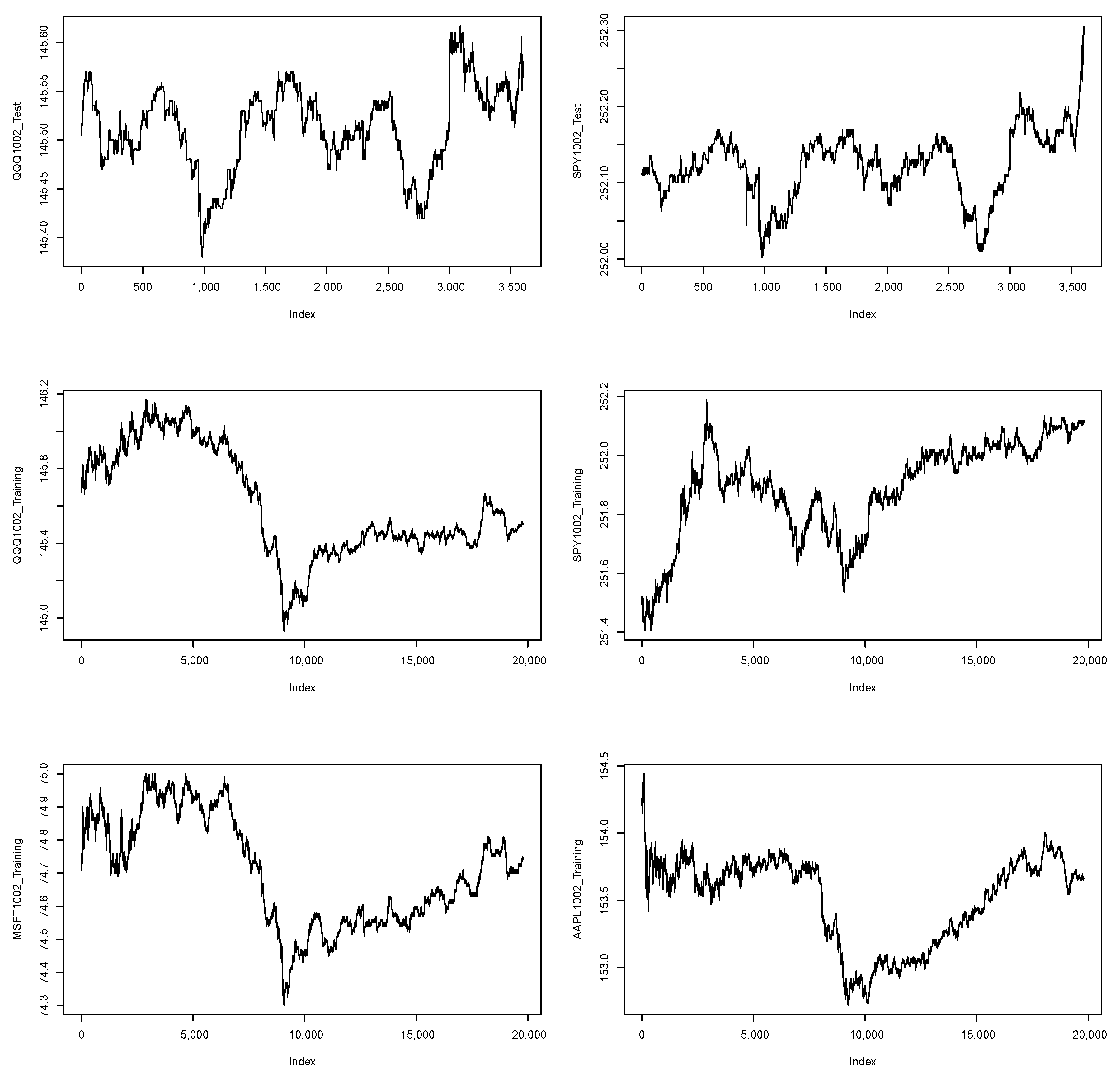
We use PowerShares QQQ Trust Series 1 (QQQ) and SPDR S&P 500 ETF Trust (SPY). These are exchange-traded funds incorporated in the USA. QQQ ETF tracks the performance of the Nasdaq 100 Index. It holds large-cap U.S. stocks and tends to focus on the technology and consumer sector. The holdings are weighted by market capitalization. As of 6 October 2017, there were 107 holding companies. The top three holding companies are Apple Inc., Austin, TX, USA (AAPL, 11.57%), Microsoft Corp., Redmond, WA, USA (MSFT, 8.44%), and Amazon.com, Inc., Seattle, WA, USA (AMZN, 6.86%). SPY ETF tracks the S&P 500 Index. The trust consists of a portfolio representing all 500 stocks in the S&P 500 Index. It holds predominantly large-cap U.S. stocks. It is structured as a unit investment trust and pays dividends on a quarterly basis. The holdings are weighted by market capitalization. As of 6 October 2017, the top three holding companies were Apple Inc., Austin, TX, USA (AAPL, 3.67%), Microsoft Corp., Redmond, WA, USA (MSFT, 2.68%), and Facebook Inc., Menlo Park, CA, USA) Class A (FB, 1.87%).

We collected daily second-level QQQ ETF, SPY ETF, MSFT, and AAPL price time series for this study. The QQQ ETF price time series and SPY ETF price time series are used as the vector-based ETF price ${\mathit{p}}_t$. The MSFT and AAPL stock price time series are used as the vector-based predictive variable ${\mathit{x}}_t$. The collection period is the daily trading time from 9:30 a.m. to 4:00 p.m. (Eastern Time) to ensure a high liquid market. We divided QQQ ETF and SPY ETF time series into two data sets: vector-based ETF price ${\mathit{p}}_t$ training data (9:30 a.m. to 3:00 p.m., which contains 19,800 s) and vector-based ETF price ${\mathit{p}}_t$ test data (3:00 p.m. to 4:00 p.m., which contains 3601 s). We use the MSFT and AAPL price time series as the vector-based predictive variables’ ${\mathit{x}}_t$ training data (9:30 a.m. to 3:00 p.m., which contains 19,800 s). We set initial wealth $w_0=10,000$ and interest rate $r=0$. Suppose that the investor’s risk tolerance is $0.000001$. We restrict $a_1$, $a_2$, $a_3$, $a_4$, and $a_5$ in $[0,1]$, s in $5,10$, and l in $30,60,90,120,180,$ and 240. We use training data to choose model parameters with the highest return. We first report the MGMA strategy performance summary for QQQ ETF and SPY ETF on training data; then, we report the MGMA strategy evaluation summary for QQQ ETF and SPY ETF on test data. Our study spans five days from 10 February 2017 to 10 June 2017. We plot second-level QQQ ETF and SPY ETF price time series on day 1 (10 February 2017) in Figure 1 as an example.

Figure 1. Case 1—Second-level QQQ ETF and SPY ETF prices time series on day 1 (10 February 2017).

The MGMA strategy performance summary for QQQ ETF and SPY ETF on day 1 (10 February 2017) to day 5 (10 June 2017); training data are provided in Table 8. The MGMA strategy evaluation summary for QQQ ETF and SPY ETF on day 1 (10 February 2017) to day 5 (10 June 2017) test data is provided in Table 9.

Table 8. Case 1—MGMA strategy performance summary for QQQ ETF and SPY ETF on day 1 (10 February 2017) to day 5 (10 June 2017) training data.

Training Data	Day time T dt	10 February 2017 9:30 a.m.–3:00 p.m. 19,800 s 1 s	10 March 2017 9:30 a.m.–3:00 p.m. 19,800 s 1 s	10 April 2017 9:30 a.m.–3:00 p.m. 19,800 s 1 s	10 May 2017 9:30 a.m.–3:00 p.m. 19,800 s 1 s	10 June 2017 9:30 a.m.–3:00 p.m. 19,800 s 1 s
$tunedparameters$	s	10	10	10	10	10
	l	180	60	240	180	120
	${\widehat{a}}_1$	0.3287	0.1250	0.0742	0.0737	0.8537
	${\widehat{a}}_2$	0.9611	0.2346	0.7111	0	0.2780
	${\widehat{a}}_3$	0.0352	0	0	1	0
	${\widehat{a}}_4$	0.7160	0	0	1	0
	${\widehat{a}}_5$	1	1	1	1	1
$backwardMA$	$E\left(W_T\right)$	10,009.49768	9,955.07379	10,001.35849	10,002.15772	9,997.54490
	$returnratio(\%)$	0.09498%	−0.44926%	0.01358%	0.02158%	−0.02455%
	$transnum$	504	1,117	421	535	589
$backwardMGMA$	$E\left(W_T\right)$	10,024.54175	9,974.19921	10,010.97889	10,015.65524	10,016.17125
	$returnratio(\%)$	0.24542%	−0.25801%	0.10979%	0.15655%	0.16171%
	$transnum$	655	1,557	534	708	794

Table 9. Case 1—MGMA strategy evaluation summary for QQQ ETF and SPY ETF on day 1 (10 February 2017) to day 5 (10 June 2017) test data.

test data	day time T dt	10 February 2017 3:00 p.m.–4:00 p.m. 3601 s 1 s	10 March 2017 3:00 p.m.–4:00 p.m. 3601 s 1 s	10 April 2017 3:00 p.m.–4:00 p.m. 3601 s 1 s	10 May 2017 3:00 p.m.–4:00 p.m. 3601 s 1 s	10 June 2017 3:00 p.m.–4:00 p.m. 3601 s 1 s
$tunedparameters$	s	10	10	10	10	10
	l	180	60	240	180	120
	${\widehat{a}}_1$	0.3287	0.1250	0.0742	0.0737	0.8537
	${\widehat{a}}_2$	0.9611	0.2346	0.7111	0	0.2780
	${\widehat{a}}_3$	0.0352	0	0	1	0
	${\widehat{a}}_4$	0.7160	0	0	1	0
	${\widehat{a}}_5$	1	1	1	1	1
$forwardMA$	$E\left(W_T\right)$	10,006.66819	9990.21402	9998.84086	10,003.58666	10,001.47801
	$returnratio(\%)$	0.06668%	−0.09786%	−0.01159%	0.03587%	0.01478%
	$transnum$	67	210	85	92	111
$forwardMGMA$	$E\left(W_T\right)$	10,008.53428	9991.06108	10,000.43623	10,008.31762	9999.77159
	$returnratio(\%)$	0.08534%	−0.08939%	0.00436%	0.08318%	−0.00228%
	$transnum$	82	318	127	120	141

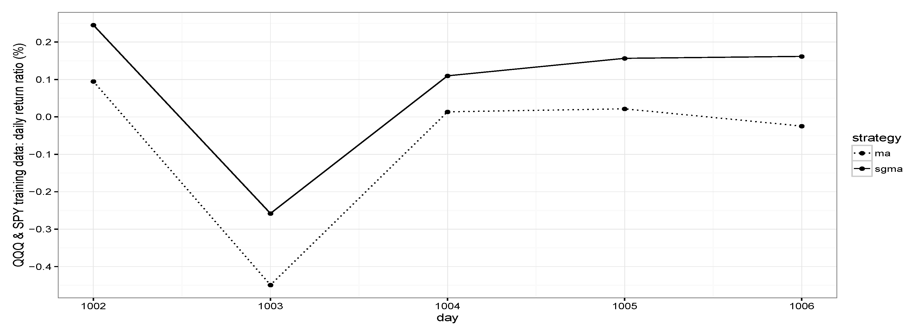
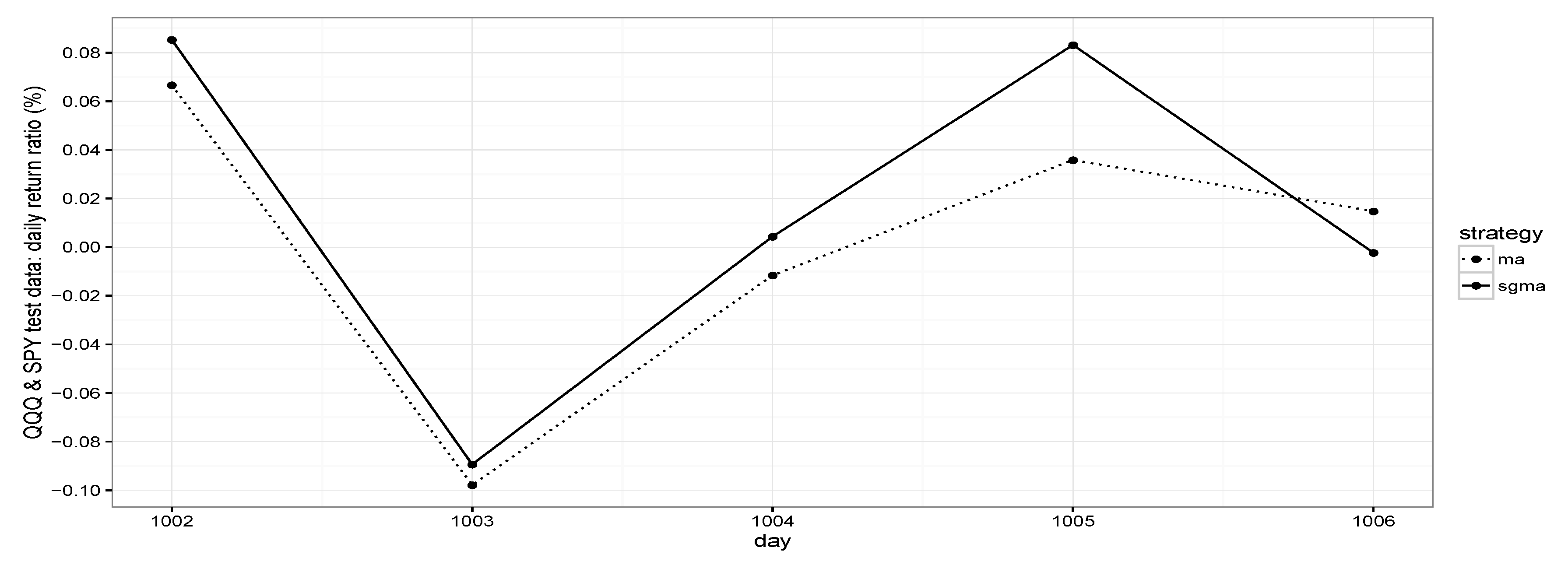
Note that the MGMA strategy in general can outperform the MA strategy for both backward investments in training data and forward investments in test data. For example, for day 1 (10 February 2017), the MGMA strategy can increase the daily return ratio from $0.09498\%$ to $0.24542\%$ on training data, which equals an increase in annual return ratio of $46.1\%$; the MGMA strategy can increase the daily return ratio from $0.06668\%$ to $0.08534\%$ on test data, which equals an increase in annual return ratio of $4.8\%$.

The MGMA strategy performance summary for QQQ ETF and SPY ETF on day 1 (10 February 2017) to day 5 (10 June 2017); training data are provided in Figure 2. The MGMA strategy evaluation summary for QQQ ETF and SPY ETF on day 1 (10 February 2017) to day 5 (10 June 2017) test data is provided in Figure 3.

Figure 2. Case 1—MGMA strategy performance summary plot for QQQ ETF and SPY ETF on day 1 (10 February 2017) to day 5 (10 June 2017) training data.

Figure 3. Case 1—MGMA strategy evaluation summary plot for QQQ ETF and SPY ETF on day 1 (10 February 2017) to day 5 (10 June 2017) test data.

6.3. Case 2: MGMA Strategy on High-Frequency Exchange-Traded Fund in Asian Market

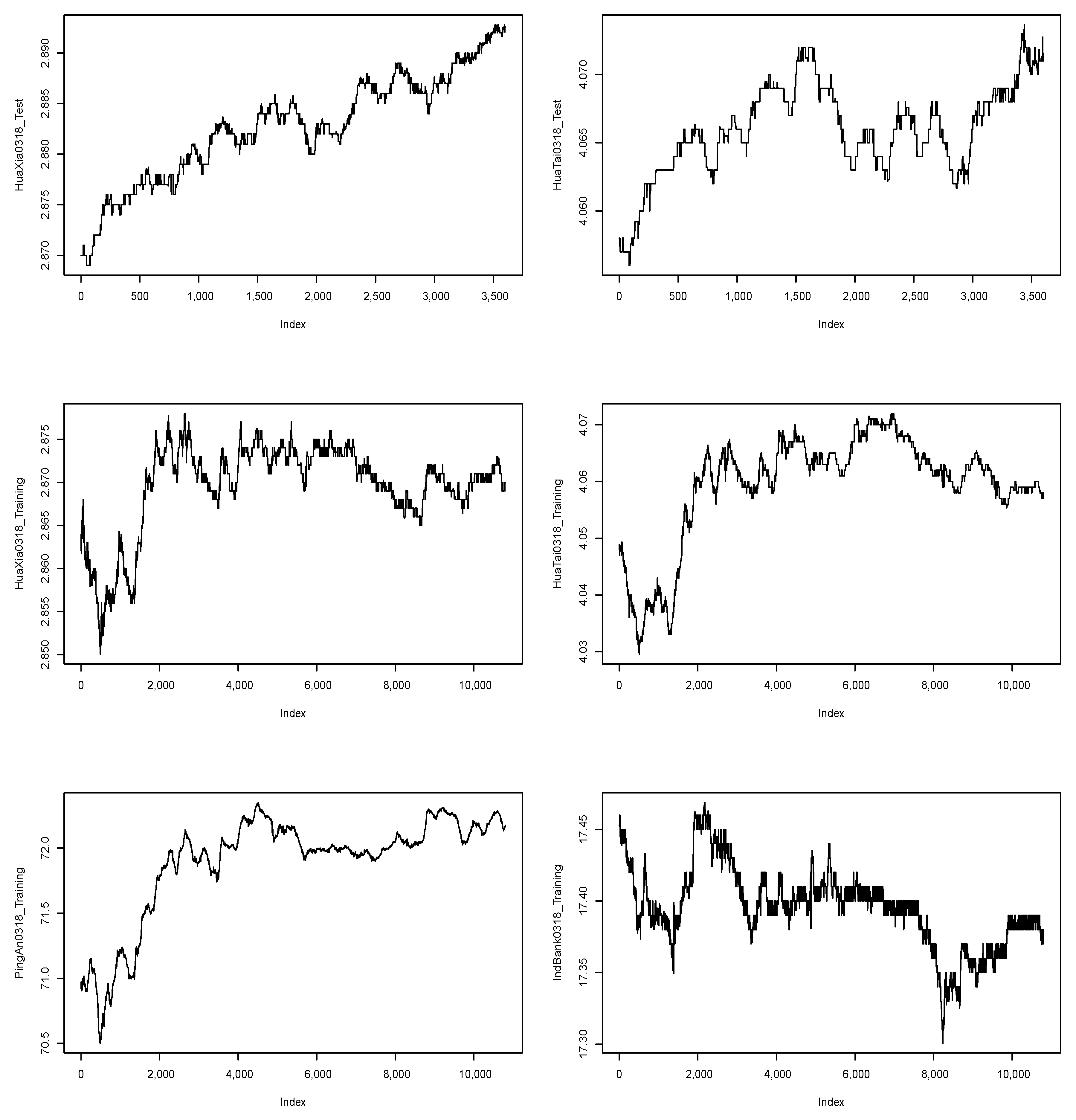
We use the China 50 ETF (HuaXia) and Huatai-Pinebridge CSI 300 ETF (HuaTai). These are exchange-traded funds incorporated in China. The China 50 ETF (HuaXia) tracks the performance of the Shanghai Stock Exchange 50 Index (the SSE 50 Index). The holdings are weighted by market capitalization. As of 22 March 2018, the top five holding companies are PingAn Insurance Group, Shenzhen, China (PingAn, 12.30%), China Merchants Bank Co Ltd., Shenzhen, China (CMB, 5.65%), Kweichow Moutai Co Ltd., Zunyi China (600519, 5.41%), Industrial Bank Co Ltd., Fuzhou, China(IndBank, 4.81%), and China Minsheng Banking Corp Ltd., Beijing, China (CMAKY, 4.45%). The Huatai-Pinebridge CSI 300 ETF (HuaTai) is a capitalization-weighted stock market index designed to replicate the performance of the top 300 stocks traded in the Shanghai and Shenzhen stock exchange. As of 22 March 2018, the top three holding companies are PingAn Insurance Group, Shenzhen, China (PingAn, 4.17%), China Merchants Bank Co Ltd., Shenzhen, China (CMB, 2.34%), and Industrial Bank Co Ltd., Fuzhou, China (IndBank, 2.34%).

We collected daily second-level HuaXia ETF, HuaTai ETF, PingAn and IndBank price time series for this study. The HuaXia ETF price time series and HuaTai ETF price time series are used as the vector-based ETF price ${\mathit{p}}_t$. The PingAn and IndBank stock price time series are used as the vector-based predictive variable ${\mathit{x}}_t$. The collection period is the daily trading time from 8:30 p.m. to 2:00 a.m. (Eastern Time) to ensure a highly liquid market. Note that there is a break time from 10:30 p.m. to 0:00 a.m. (Eastern Time) for the Asian Market. We divide the HuaXia ETF and HuaTai ETF time series into two data sets: vector-based ETF price ${\mathit{p}}_t$ training data (8:30 p.m. to 10:30 p.m. and 0:00 a.m. to 1:00 a.m., which contains 10,800 s) and vector-based ETF price ${\mathit{p}}_t$ test data (1:00 a.m. to 2:00 a.m., which contains 3601 s). We use the PingAn and IndBank price time series as vector-based predictive variable ${\mathit{x}}_t$ training data (8:30 p.m. to 10:30 p.m. and 0:00 a.m. to 1:00 a.m., which contains 10,800 s). We set initial wealth $w_0=10,000$ and interest rate $r=0$. Suppose that the investor’s risk tolerance is $0.0005$. We restrict $a_1$, $a_2$, $a_3$, $a_4$, and $a_5$ in $[0,1]$, s in $5,10$, and l in $30,60,90,120,180,$ and 240. We use training data to choose model parameters with the highest return. We first report the MGMA strategy performance summary for HuaXia ETF and HuaTai ETF on training data; then, we report the MGMA strategy evaluation summary for HuaXia ETF and HuaTai ETF on test data. Our study spans five days from 18 March 2018 to 22 March 2018. We plot the second-level HuaTai ETF and HuaXia ETF price time series on day 1 (18 March 2018) in Figure 4 as an example.

Figure 4. Case 2—Second-level HuaXia ETF and HuaTai ETF prices time series on day 1 (18 March 2018).

The MGMA strategy performance summary for HuaXia ETF and HuaTai ETF on day 1 (18 March 2018) to day 5 (22 March 2018) training data is provided in Table 10. The MGMA strategy evaluation summary for HuaXia ETF and Huatai ETF on day 1 (18 March 2018) to day 5 (22 March 2018) test data is provided in Table 11.

Table 10. Case 2—MGMA strategy performance summary for HuaXia ETF and HuaTai ETF on day 1 (18 March 2018) to day 5 (22 March 2018) training data.

training data	day time T dt	18 March 2018 8:30 p.m.–1:00 a.m. 10,800 s 1 s	19 March 2018 8:30 p.m.–1:00 a.m. 10,800 s 1 s	20 March 2018 8:30 p.m.–1:00 a.m. 10,800 s 1 s	21 March 2018 8:30 p.m.–1:00 a.m. 10,800 s 1 s	22 March 2018 8:30 p.m.–1:00 a.m. 10,800 s 1 s
$tunedparameters$	s	10	10	10	10	10
	l	30	30	30	30	30
	${\widehat{a}}_1$	1	1	1	1	1
	${\widehat{a}}_2$	1	1	1	1	1
	${\widehat{a}}_3$	1	1	1	1	1
	${\widehat{a}}_4$	1	1	1	1	1
	${\widehat{a}}_5$	1	1	1	1	1
$backwardMA$	$E\left(W_T\right)$	9697.42479	9742.02916	9483.70570	9654.20256	9645.70242
	$returnratio(\%)$	−3.02575%	−2.57971%	−5.16294%	−3.45797%	−3.54298%
	$transnum$	837	833	1043	861	917
$backwardMGMA$	$E\left(W_T\right)$	10,015.85838	10,053.51711	9945.74085	9873.99072	9961.93758
	$returnratio(\%)$	0.15858%	0.53517%	−0.54259%	−1.26009%	−0.38062%
	$transnum$	869	852	1056	914	1013

Table 11. Case 2—MGMA strategy evaluation summary for HuaXia ETF and HuaTai ETF on day 1 (18 March 2018) to day 5 (22 March 2018) test data.

test data	day time T dt	18 March 2018 1:00 a.m.–2:00 a.m. 3601 s 1 s	19 March 2018 1:00 a.m.–2:00 a.m. 3601 s 1 s	20 March 2018 1:00 a.m.–2:00 a.m. 3601 s 1 s	21 March 2018 1:00 a.m.–2:00 a.m. 3601 s 1 s	22 March 2018 1:00 a.m.–2:00 a.m. 3601 s 1 s
$tunedparameters$	s	10	10	10	10	10
	l	30	30	30	30	30
	${\widehat{a}}_1$	1	1	1	1	1
	${\widehat{a}}_2$	1	1	1	1	1
	${\widehat{a}}_3$	1	1	1	1	1
	${\widehat{a}}_4$	1	1	1	1	1
	${\widehat{a}}_5$	1	1	1	1	1
$forwardMA$	$E\left(W_T\right)$	9958.09171	9873.56029	9825.82477	9832.73198	10,049.94455
	$returnratio(\%)$	−0.41908%	−1.26440%	−1.74175%	−1.67268%	0.49945%
	$transnum$	270	317	325	311	252
$forwardMGMA$	$E\left(W_T\right)$	10,075.23280	10,001.72750	9913.81940	9988.70100	10,049.94455
	$returnratio(\%)$	0.75233%	0.01728%	−0.86181%	−0.11299%	0.47835%
	$transnum$	274	321	350	317	289

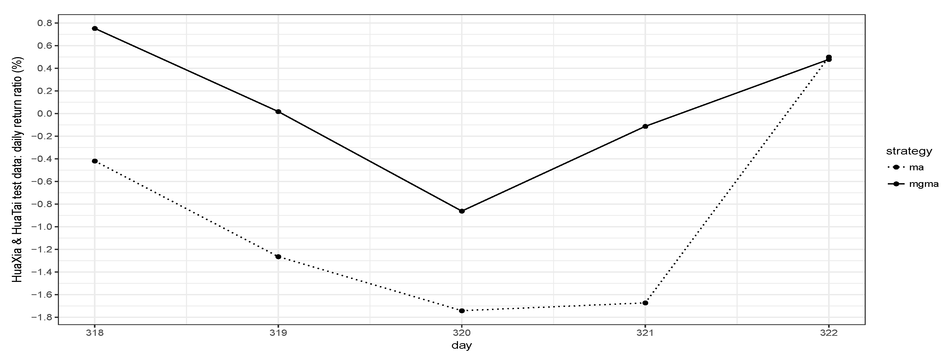
Note that the MGMA strategy in general can outperform the MA strategy for both backward investments on training data and forward investment on test data. Note that the optimal short-lag s, long-lag l, and allocation parameters $a_1^{*}$ to $a_5^{*}$ are all the same for 5 days, which might suggest that it is possible to use fixed parameters for MGMA strategy in reality.

The MGMA strategy performance summary for HuaXia ETF and HuaTai ETF on day 1 (18 March 2018) to day 5 (22 March 2018) training data is provided in Figure 5. The MGMA strategy evaluation summary for HuaXia ETF and HuaTai ETF on day 1 (18 March 2018) to day 5 (22 March 2018) test data is provided in Figure 6.

Figure 5. Case 2—MGMA strategy performance summary plot for HuaXia ETF and HuaTai ETF on day 1 (18 March 2018) to day 5 (22 March 2018) training data.

Figure 6. Case 2—MGMA strategy evaluation summary plot for HuaXia ETF and HuaTai ETF on day 1 (18 March 2018) to day 5 (22 March 2018) test data.

7. Conclusions

In this paper, we propose a multiasset generalized moving average crossover (MGMA) strategy. Our study demonstrates that the MGMA strategy can provide more investment options with the investor’s risk tolerance. The MGMA strategy can solve the well-known problem for the MA strategy for a multiasset portfolio. Simulation studies demonstrate that the MGMA strategy can increase both the investor’s expected utility of wealth and the investor’s expected wealth. Two high-frequency ETF real-time examples from the North American market and Asian market demonstrate that the MGMA strategy can outperform the MA strategy for both backward investment on training data and forward investment on test data. The MGMA strategy has built the foundation for reconciling the moving average technique with the portfolio allocation strategy for multiple assets. In the future, we would like to extend the algorithm for adaptive or online prediction in order to go beyond the current reactionary nature. While this approach is proposed for optimizing asset allocation, it can also be used to create a general framework for analyzing the relative importance or impact of a particular repeated measured index in a multiple time series setting. It could have broad applications in climate change or healthcare.