A Two-Step Lagrange–Galerkin Scheme for the Shallow Water Equations with a Transmission Boundary Condition and Its Application to the Bay of Bengal Region—Part I: Flat Bottom Topography

Abstract

A two-step Lagrange–Galerkin scheme for the shallow water equations with a transmission boundary condition (TBC) is presented. First, we show the experimental order of convergence to see the second-order accuracy in time realized by the two-step methods for conservative and non-conservative material derivatives along the trajectory of fluid particles. Second, we observe the effect of the TBC in a simple domain, and the artificial reflection is removed significantly when the wave touches the TBC. Third, we apply the scheme to a practical domain with islands, namely, the Bay of Bengal region, and observe the effect of the TBC again for the practical domain; the artificial reflections are removed significantly from the transmission boundaries on open sea boundaries. We also study the effect of a position of an open sea boundary with the TBC and reveal that it is sufficiently small to neglect. The numerical results in this study show that the scheme has the following properties: (i) the same advantages of Lagrange–Galerkin methods (the CFL-free robustness for convection-dominated problems and the symmetry of the matrices for the system of linear equations); (ii) second-order accuracy in time by the two-step methods; (iii) mass preservation of the function for the water level from the reference height (until the contact with the transmission boundaries of the wave); and (iv) no significant artificial reflection from the transmission boundaries. The numerical results by the scheme presented in this paper are for the flat bottom topography of the domain. In the next part of this work, Part II, the scheme will be applied to rapidly varying bottom surfaces and a real bottom topography of the Bay of Bengal region.

1. Introduction

The system of shallow water equations (SWEs) is one of the most common models for describing fluid flow in rivers, channels, estuaries, and coastal areas, and is often used for simulating tsunamis and storm surges in oceanic phenomena. Natural disasters like tsunamis, cyclones, and storm surges cause a tremendous loss of lives and properties in the coastal areas in several regions. According to [1], statistics show that about 5% of the global tropical cyclones form over the Bay of Bengal, and, on average, five to six storms form in this region every year, but with 80% of the global casualties. The significant factors behind the heavy casualties are the shallow coastal water, thickly populated low-lying islands, highly curved coastal and island boundaries, river discharge, high astronomical tidal range, and favorable cyclone track, cf. [2] and Figure 1. That is why an effective storm surge prediction model and method are highly desired for the coastal region of Bangladesh to minimize the resulting damage from storm surges.

Figure 1. The Bay of Bengal region.

Studies focusing on the Bay of Bengal region are found in [1,2,3,4,5,6,7,8] and references therein. Almost all the researchers implemented SWEs with a radiation-type boundary condition for open sea boundaries. Although for real problems, the finite element method is more suitable than the finite difference method because of the advantages of handling complex physical domains, geometries, or boundary conditions, as far as we know, there is no study to solve SWEs employing a transmission boundary condition (TBC) for the Bay of Bengal region using the finite element method except [9,10].

Since a bounded computational domain is needed to compute the SWEs in a practical coastal region, e.g., the Bay of Bengal, we set an artificial boundary in the open sea, called the open boundary, which is a part of the boundary of the domain. Let $u={(u_1,u_2)}^{\top }$ be the velocity (averaged in $x_3$-direction), $\varphi (=\eta +\zeta )$ the total wave height, $\eta$ the water level from the reference height, and $\zeta ($>$0)$ the depth of the water level from the reference height. On the coastal boundary, it is natural to have the reflection, which is realized by the Dirichlet boundary condition, $u=0$, and, on the open boundary, an artificial boundary condition is required so that the wave passes through the boundary without any reflection, as the boundary is set artificially on the open sea. Most open boundary conditions proposed in the literature are based on or modifications of the Sommerfeld radiation boundary condition (RBC) [11] whose typical form is

$$u=\sqrt{g/\zeta }\eta n$$

(1)

for the gravity constant $g($>$0)$ and the outward unit normal vector n. The condition (1) is derived by considering the SWEs in one-dimensional space essentially and assuming that the velocity u on the open boundary is $u=V\eta /\zeta n$ for the wave propagation speed V and that V is given by $V=\sqrt{g\zeta }$. Due to some limitations of the RBC for oblique flows, many researchers suggested and implemented modified boundary conditions for open boundaries similar to the RBC, cf., e.g., [12,13,14]. Kanayama and Dan [15] also employed an open boundary condition of the form,

$$u=c_0\sqrt{g\zeta }\eta /\varphi n$$

(2)

for a constant $c_0($>$0)$, which removes the artificial reflection from the open boundary significantly. The condition (2) is comparable to the RBC as Equation (2) is obtained by replacing $\zeta$ with ${\varphi }^2/\zeta$ in Equation (1), where the relation $\zeta \approx {\varphi }^2/\zeta \approx \varphi$ holds if $\left|\eta \right|\ll \zeta$ is satisfied. In fact, the numerical results by the TBC and the RBC are similar, cf. Appendix B. On the other hand, the TBC is more reasonable than the RBC for the theoretical stability study of the system of the SWEs from the viewpoint of energy as presented in Murshed et al. [9] and Murshed [10], while it is still a partial study (but practically useful), cf. Remark 6 for a brief review of the theoretical results. Based on the stability study, we employ the TBC in this paper and observe the effect of the TBC (or the RBC) for the passing wave in addition to the effect of the Dirichlet boundary condition for the reflection wave. These observations are basic but necessary for the development of a scheme for SWEs.

The system of the SWEs consists of two equations, a pure convection equation for the total wave height and a modified Navier–Stokes momentum equation for the velocity derived by taking the average of function values in $x_3$-direction, cf. [9,16], which include the material derivatives in conservative and non-conservative forms, respectively. For a time step size $\Delta t>0$, let $t^n := n\Delta t$. The so-called Lagrange–Galerkin method is the finite element method combined with the idea of the method of characteristics; the non-conservative and conservative material derivatives are discretized as, for a scalar-valued function $\varphi$ and a velocity u, cf., e.g., [17,18,19,20],

$$\begin{array}{cc}\hfill \left[\frac{\partial \varphi }{\partial t}+u·\nabla \varphi \right](x,t^n)& =\frac{{\varphi }^n\left(x\right)-{\varphi }^{n-1}(x-u^n\left(x\right)\Delta t)}{\Delta t}+O(\Delta t),\hfill \\ \hfill \left[\frac{\partial \varphi }{\partial t}+\nabla ·\left(u\varphi \right)\right](x,t^n)& =\frac{{\varphi }^n\left(x\right)-{\varphi }^{n-1}(x-u^n\left(x\right)\Delta t){\gamma }^n\left(x\right)}{\Delta t}+O(\Delta t),\hfill \end{array}$$

respectively, which are first-order approximations in time, where $x-u^n\left(x\right)\Delta t$ is an upwind point of x with respect to $u^n\left(x\right)$ and ${\gamma }^n$ is the Jacobian determinant of the mapping $x-u^n\left(x\right)\Delta t$. In general, the Lagrange–Galerkin method has two advantages; (i) the CFL-free robustness for convection-dominated problems and (ii) the symmetry of the resulting coefficient matrices for the system of linear equations. In addition to the four pioneering works above, many authors have proposed the ideas of this type of approximation in the context of the finite element method, cf. [21,22,23,24,25,26,27,28,29,30,31,32,33,34,35,36,37,38,39,40,41,42,43,44,45,46,47,48] and references therein. When we focus on the SWEs, to the best of our knowledge, Murshed et al. [9] and Murshed [10] firstly solved the SWEs with a TBC by a (single-step) Lagrange–Galerkin scheme of first-order in time for a flat bottom topography. Recently, a two-step mass-preserving Lagrange–Galerkin scheme of second order in time for conservative convection-diffusion problems has been proposed and analyzed with error estimates in [49].

In this paper, we present a new two-step Lagrange–Galerkin scheme to solve the SWEs together with a TBC, which is of second order in time and maintains the two advantages of the Lagrange–Galerkin methods, i.e., the CFL-free robustness and the symmetry of the resulting matrices. The two material derivatives are discretized based on the ideas of two-step methods proposed for the non-conservative form in [17,21,24,40] and the conservative form in [49]. Firstly, preparing an artificial exact solution, we observe our scheme’s experimental order of convergence (EOC) to see the second-order accuracy in time on a simple (square) domain. Since long (real-)time computations on a mesh refined locally are needed in practical problems, the CFL-free second-order accuracy in time of our scheme is a significant advantage, enabling us to employ a more extensive time increment compared with first-order numerical methods. Secondly, we observe the effect of the TBC on a simple (square) domain, and the artificial reflections are kept from the Dirichlet boundaries and removed significantly from the transmission boundaries. Thirdly, our scheme is applied to the Bay of Bengal region, which is non-convex, includes islands, and is, therefore, a complex domain. We again observe the effect of the TBC for this realistic domain. The artificial reflections are removed significantly from the transmission boundaries, which are set on open sea boundaries. We also study the effect of a position of an open sea boundary with the TBC and reveal that it is sufficiently small to neglect. In [9], energy estimates for the SWEs were given, where the $L^2$-norm of the water level from the reference height was an important value related to the potential energy. Focusing on the energy and the mass of the water level function, we observe the $L^2$-norm and the mass of the water level function, which show the effectiveness of the TBC.

From the computations, we show that our new scheme has the following properties; (i) the same advantages of Lagrange–Galerkin methods; (ii) second-order accuracy in time; (iii) mass preservation of the function of the water level from the reference height (until the contact with the transmission boundaries of the wave); and (iv) no significant artificial reflection from the transmission boundaries. We mention again that the TBC is employed in this paper based on the theoretical stability study in [9,10], while the numerical results by the TBC and the RBC are similar.

All of the numerical results in this paper, Part I, are for the flat bottom topography, and the non-homogeneous bottom topography will be studied in our forthcoming paper, Part II.

The outline of this paper is as follows. Section 2 presents a two-step Lagrange–Galerkin scheme for the SWEs together with a TBC, which is of second order in time. In Section 3, numerical results for simple square domains are shown to observe the second-order accuracy in time and the effect of TBC. In Section 4, our scheme is applied to the Bay of Bengal region, where the domain is non-convex and complex. In Section 5, conclusions are given. The data for choosing the constant $c_0$ required in the TBC and a comparison of the TBC with the RBC are given in Appendix A and Appendix B, respectively.

2. A Two-Step Lagrange–Galerkin Scheme

We introduce some notations to be used in this paper. $\Omega$ is a bounded spatial domain in ${\mathbb{R}}^2$, $\Gamma := \partial \Omega$ is the boundary of $\Omega$, and $(0,T)$ is a temporal domain in ${\mathbb{R}}_{+}(:=\{x\in \mathbb{R};x>0\})$ for a positive constant T. We use the Lebesgue space $L^p(\Omega )(p\in [1,\infty ])$ and the Sobolev space $H^1(\Omega )$. For any normed space X with its norm ${\parallel ·\parallel }_X$, we define function spaces $C^0([0,T];X)$ and $L^{\infty }(0,T;X)$ consisting of X-valued functions in $C^0\left([0,T]\right)$ and $L^{\infty }(0,T)$, respectively. Let $(·,·)$ be the inner product in $L^2(\Omega )$, i.e., $(f,g) := {\int }_{\Omega }f\left(x\right)g\left(x\right)dx$ for $f,g\in L^2(\Omega )$. We employ the same notation $(·,·)$ to represent the $L^2(\Omega )$ inner product for scalar-, vector-, and matrix-valued functions. Let $A:B$ be the tensor product defined by $A:B := {\sum }_{i,j=1}^2{A}_{ij}{B}_{ij}=\mathrm{tr}\left(A{B}^{\top }\right)$ for $A,B\in {\mathbb{R}}^{2\times 2}$.

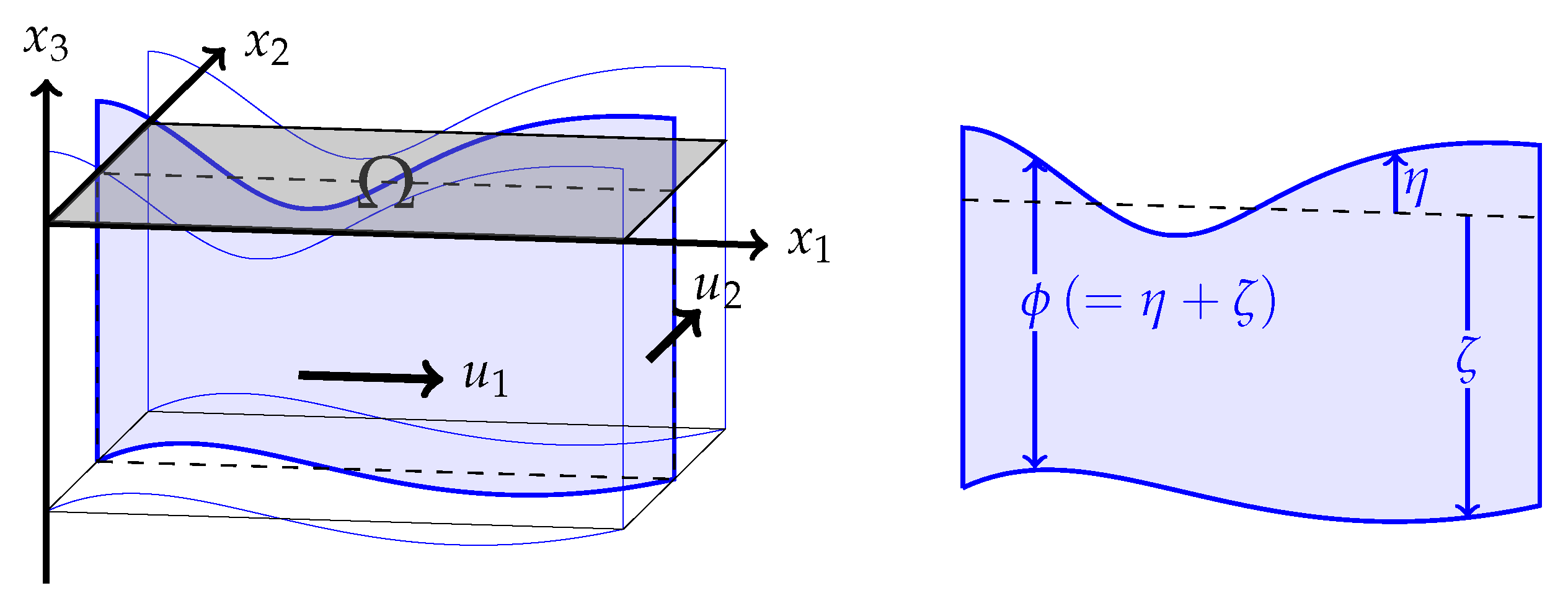
2.1. Statement of the Problem

Our problem is to find $(\varphi ,u):\Omega \times (0,T)\to \mathbb{R}\times {\mathbb{R}}^2$ such that

$$\begin{array}{cccc}\hfill \frac{\partial \varphi }{\partial t}+\nabla ·\left(u\varphi \right)& =f\hfill & \hfill & \mathrm{in}\Omega \times (0,T),\hfill \end{array}$$

(3a)

$$\begin{array}{ccc}\hfill \rho \varphi \left[\frac{\partial u}{\partial t}+(u·\nabla )u\right]-2\mu \nabla ·\left(\varphi D\left(u\right)\right)+\rho g\varphi \nabla \eta =F& \hfill & \mathrm{in}\Omega \times (0,T),\hfill \end{array}$$

(3b)

$$\begin{array}{cccc}\hfill \varphi & =\eta +\zeta \hfill & \hfill & \mathrm{in}\Omega \times (0,T),\hfill \end{array}$$

(3c)

$$\begin{array}{cccc}\hfill u& =0\hfill & \hfill & \mathrm{on}{\Gamma }_{\mathrm{D}}\times (0,T),\hfill \end{array}$$

(3d)

$$\begin{array}{cccc}\hfill u& =c_0\sqrt{g\zeta }\frac{\eta }{\varphi }n\hfill & \hfill & \mathrm{on}{\Gamma }_{\mathrm{T}}\times (0,T),\hfill \end{array}$$

(3e)

$$\begin{array}{cccc}\hfill (\varphi ,u)& =({\varphi }^0,u^0)\hfill & \hfill & \mathrm{in}\Omega ,\mathrm{at}t=0,\hfill \end{array}$$

(3f)

where the total wave height and the velocity are denoted by $\varphi$ and $u={(u_1,u_2)}^{\top }$, respectively, the water level from the reference height and the depth of water level from the reference height, i.e., bottom topography, are represented by $\eta :\Omega \times (0,T)\to \mathbb{R}$ and $\zeta :\Omega \to {\mathbb{R}}_{+}$, respectively, a pair of external forces is given by $(f,F):\Omega \times (0,T)\to \mathbb{R}\times {\mathbb{R}}^2$, a pair of initial values is given by $({\varphi }^0,u^0):\Omega \to \mathbb{R}\times {\mathbb{R}}^2$, density and viscosity constants of water are denoted by $\rho >0$ and $\mu >0$, the gravity constant is given by $g>0$, the strain-rate tensor $D\left(u\right)$ is defined by

$$D\left(u\right):=\frac{1}{2}\left[\nabla u+{(\nabla u)}^{\top }\right],$$

and the outward unit normal vector is denoted by $n:\Gamma \to {\mathbb{R}}^2$, cf. Figure 2. We suppose that the boundary $\Gamma$ is divided into two non-overlapping parts, ${\Gamma }_{\mathrm{D}}$ and ${\Gamma }_{\mathrm{T}}$, i.e., $\overline{\Gamma }={\overline{\Gamma }}_{\mathrm{D}}\cup {\overline{\Gamma }}_{\mathrm{T}}$ and ${\Gamma }_{\mathrm{D}}\cap {\Gamma }_{\mathrm{T}}=\varnothing$, where the subscripts “$\mathrm{D}$” and “$\mathrm{T}$” imply Dirichlet and transmission boundaries, respectively. A positive constant $c_0$ is chosen suitably to remove the artificial reflection, and, throughout this paper, we employ $c_0=0.9$, which is determined based on numerical experiments given in Appendix A. We consider homogeneous flat bottom topography in this paper, Part I, and non-homogeneous bottom topography in our forthcoming paper, Part II.

Figure 2. Diagrams for the problem; left: the domain $\Omega$ and the velocity $u={(u_1,u_2)}^{\top }$; right: the total wave height $\varphi =\eta +\zeta$.

2.2. Presentation of the Scheme

Let $\Psi := L^2(\Omega )$, $Y := H^1{(\Omega )}^2$,

$$V\left(G\right) := \left\{v\in Y;v=0\mathrm{on}{\Gamma }_{\mathrm{D}}\mathrm{and}v=G\mathrm{on}{\Gamma }_{\mathrm{T}}\right\}$$

for a function $G:{\Gamma }_{\mathrm{T}}\to {\mathbb{R}}^2$, and $V := V\left(0\right)$. We introduce a $\varphi$-dependent function, $G\left(\varphi \right)=G(\varphi ;\eta ):{\Gamma }_{\mathrm{T}}\to {\mathbb{R}}^2$, defined by

$$G\left(\varphi \right)=G(\varphi ;\eta ) := c_0\sqrt{g\zeta }\frac{\eta }{\varphi }n.$$

Assume ${\varphi }^0\in \Psi$, ${\eta }^0{\varphi }^0 := -\zeta \in \Psi$ and $u^0\in V\left(G\left({\varphi }^0\right)\right)=V\left(G({\varphi }^0;{\eta }^0)\right)$. A weak formulation to problem (3) is to find $\left\{\right(\varphi ,u\left)\right(t)\in \Psi \times V(G\left(\varphi \right(t);\eta (t\left)\right));t\in (0,T\left)\right\}$ such that, for $t\in (0,T)$,

$$\begin{array}{cc}\hfill \left(\frac{\partial \varphi }{\partial t}+\nabla ·\left(u\varphi \right),\psi \right)& =(f,\psi )\forall \psi \in \Psi ,\hfill \end{array}$$

(4a)

$$\begin{array}{cc}\hfill \rho \left(\varphi \left[\frac{\partial u}{\partial t}+(u·\nabla )u\right],v\right)+a(u,v;\varphi )+b(\eta ,v;\varphi )& =(F,v)\forall v\in V,\hfill \end{array}$$

(4b)

$$\begin{array}{cc}\hfill \varphi & =\eta +\zeta ,\hfill \end{array}$$

(4c)

with the initial condition $(\varphi ,u)\left(0\right)=({\varphi }^0,u^0)\in \Psi \times V\left(G({\varphi }^0;{\eta }^0)\right)$, where the bilinear forms $a(·,·;\varphi ):Y\times Y\to \mathbb{R}$ and $b(·,·;\varphi ):\Psi \times Y\to \mathbb{R}$ are defined by

$$\begin{array}{cccc}\hfill a(u,v;\varphi ) := & 2\mu \left(\varphi D\left(u\right),D\left(v\right)\right),\hfill & \hfill b(\eta ,v;\varphi ) := & \rho g\left(\varphi \nabla \eta ,v\right).\hfill \end{array}$$

Now, we present our scheme for solving problem (3). Let ${\mathcal{T}}_h=\left\{K\right\}$ be a partition of $\overline{\Omega }$ by triangular elements, h be the maximum diameter of $K\in {\mathcal{T}}_h$, and ${\Omega }_h := \mathrm{int}\left({\cup }_{K\in {\mathcal{T}}_h}K\right)$ be an approximated domain. Although it holds that $\Omega \ne {\Omega }_h$ in general, we assume $\Omega ={\Omega }_h$ throughout the paper to avoid the complexity of introducing many symbols. We define finite element spaces, ${\Psi }_h$, $Y_h$ and $V_h\left(G\right)$, corresponding to $\Psi$, Y and $V\left(G\right)$ by

$$\begin{array}{cc}\hfill {\Psi }_h := & \{{\psi }_h\in C^0\left(\overline{\Omega }\right);{\psi }_{h|K}\in P_k\left(K\right)\forall K\in {\mathcal{T}}_h\},\hfill \\ \hfill Y_h := & \{v_h\in C^0{\left(\overline{\Omega }\right)}^2;v_{h|K}\in P_{\ell }{\left(K\right)}^2\forall K\in {\mathcal{T}}_h\},\hfill \\ \hfill V_h\left(G\right) := & \{v_h\in Y_h;v_h=0\mathrm{on}{\Gamma }_{\mathrm{D}}\mathrm{and}{v}_h=G\mathrm{on}{\Gamma }_{\mathrm{T}}\},\hfill \end{array}$$

for $k,\ell \in \mathbb{N}$, and set $V_h{V}_h := \left(0\right)$, where $P_k\left(K\right)$ is the space of polynomial functions of degree $k\in \mathbb{N}$ on $K\in {\mathcal{T}}_h$. In this paper, we employ $k=\ell =1$, and the function $G:{\Gamma }_{\mathrm{T}}\to {\mathbb{R}}^2$ is assumed to be a piecewise linear function.

Let $\Delta t$ be a time increment, $N_T := \lfloor T/\Delta t\rfloor$ a total number of time steps, and $t^n := n\Delta t$ a time at n-th time step. For $v:\Omega \to {\mathbb{R}}^2$, we define mappings $X_1\left[v\right],{\tilde{X}}_1\left[v\right]:\Omega \to {\mathbb{R}}^2$ and ${\gamma }_1\left[v\right],{\tilde{\gamma }}_1\left[v\right]:\Omega \to \mathbb{R}$ by

$$\begin{array}{cccc}\hfill X_1\left[v\right]\left(x\right) := & x-\Delta tv\left(x\right),\hfill & \hfill {\tilde{X}}_1\left[v\right]\left(x\right) := & x-2\Delta tv\left(x\right),\hfill \\ \hfill {\gamma }_1\left[v\right]\left(x\right) := & det\left(\frac{\partial X_1\left[v\right]}{\partial x}\left(x\right)\right),\hfill & \hfill {\tilde{\gamma }}_1\left[v\right]\left(x\right) := & det\left(\frac{\partial {\tilde{X}}_1\left[v\right]}{\partial x}\left(x\right)\right).\hfill \end{array}$$

For ${\left\{{\varphi }^n\right\}}_{n=0}^{N_T}$ and ${\left\{u^n\right\}}_{n=0}^{N_T}$, we define an operator ${\mathcal{A}}_{\Delta t}\left[u\right]{\varphi }^n$ by, for $n=1,\dots ,N_T$,

$$\begin{array}{cc}\hfill {\mathcal{A}}_{\Delta t}\left[u\right]{\varphi }^n := & \left\{\begin{array}{cccc}\hfill & {\mathcal{A}}_{\Delta t}^{\left(1\right)}\left[u\right]{\varphi }^n\hfill & \hfill & (n=1),\hfill \\ \hfill & {\mathcal{A}}_{\Delta t}^{\left(2\right)}\left[u\right]{\varphi }^n\hfill & \hfill & (n\ge 2),\hfill \end{array}\right.\hfill \end{array}$$

where

$$\begin{array}{cc}\hfill {\mathcal{A}}_{\Delta t}^{\left(1\right)}\left[u\right]{\varphi }^n := & \frac{{\varphi }^n-{\varphi }^{n-1}\circ X_1\left[u^{n-1}\right]{\gamma }_1\left[u^{n-1}\right]}{\Delta t},\hfill \\ \hfill {\mathcal{A}}_{\Delta t}^{\left(2\right)}\left[u\right]{\varphi }^n := & \frac{3{\varphi }^n-4{\varphi }^{n-1}\circ X_1\left[u^{n\ast }\right]{\gamma }_1\left[u^{n\ast }\right]+{\varphi }^{n-2}\circ {\tilde{X}}_1\left[u^{n\ast }\right]{\tilde{\gamma }}_1\left[u^{n\ast }\right]}{2\Delta t}.\hfill \end{array}$$

The composition of functions is represented by the symbol ∘, i.e.,

$$\left(\psi \circ X_1\left[v\right]\right)\left(x\right)=\psi \left(X_1\left[v\right]\left(x\right)\right),$$

and the function $u^{n\ast }:\Omega \to {\mathbb{R}}^2$ is defined by

$$u^{n\ast } := 2u^{n-1}-u^{n-2},$$

which is a second-order temporal approximation of $u^n$ if u is sufficiently smooth. We also define, for ${\left\{w^n\right\}}_{n=0}^{N_T}$,

$${\mathcal{B}}_{\Delta t}\left[w\right]u^n := \left\{\begin{array}{ccc}{\mathcal{B}}_{\Delta t}^{\left(1\right)}\left[w\right]u^n& & (n=1),\\ {\mathcal{B}}_{\Delta t}^{\left(2\right)}\left[w\right]u^n& & (n\ge 2),\end{array}\right.$$

where

$$\begin{array}{cc}\hfill {\mathcal{B}}_{\Delta t}^{\left(1\right)}\left[w\right]u^n := & \frac{u^n-u^{n-1}\circ X_1\left[w^{n-1}\right]}{\Delta t},\hfill \\ \hfill {\mathcal{B}}_{\Delta t}^{\left(2\right)}\left[w\right]u^n := & \frac{3u^n-4u^{n-1}\circ X_1\left[w^{n\ast }\right]+u^{n-2}\circ {\tilde{X}}_1\left[w^{n\ast }\right]}{2\Delta t}.\hfill \end{array}$$

The two-step Lagrange–Galerkin scheme is to find $\{({\varphi }_h^n,u_h^n)\in {\Psi }_h\times V_h\left(G({\varphi }_h^n;{\eta }_h^n)\right);$$n=1,\dots ,N_T\}$ such that, for $n=1,2,\dots ,N_T$,

$$\begin{array}{ccc}\hfill \left({\mathcal{A}}_{\Delta t}\left[u_h\right]{\varphi }_h^n,{\psi }_h\right)& =\left(f^n,{\psi }_h\right)\hfill & \hfill \forall {\psi }_h\in {\Psi }_h,\end{array}$$

(5a)

$$\begin{array}{ccc}\hfill \rho \left({\varphi }_h^n{\mathcal{B}}_{\Delta t}\left[u_h\right]u_h^n,v_h\right)+a\left(u_h^n,v_h;{\varphi }_h^n\right)+b\left({\eta }_h^n,v_h;{\varphi }_h^n\right)& =\left(F^n,v_h\right)\hfill & \hfill \forall v_h\in V_h,\end{array}$$

(5b)

$$\begin{array}{cc}\hfill {\varphi }_h^n& ={\eta }_h^n+{\Pi }_h\zeta ,\hfill \end{array}$$

(5c)

with an initial condition

$$\begin{array}{c}\hfill \left({\varphi }_h^0,u_h^0\right)=\left({\Pi }_h{\varphi }^0,{\Pi }_h{u}^0\right)\in {\Psi }_h\times Y_h,\end{array}$$

(5d)

where the Lagrange interpolation operator is denoted by ${\Pi }_h:C\left(\overline{\Omega }\right)\to {\Psi }_h$, which is also used for the vector-valued function $u^0$, i.e., ${\Pi }_h{u}^0\in Y_h$.

Remark 1.

Scheme (5) is equivalent to

$$\begin{array}{ccc}\hfill \left(\frac{{\varphi }_h^n-{\varphi }_h^{n-1}\circ X_1\left[u_h^{n-1}\right]{\gamma }_1\left[u_h^{n-1}\right]}{\Delta t},{\psi }_h\right)& =\left(f^n,{\psi }_h\right)\hfill & \hfill \forall {\psi }_h\in {\Psi }_h,\\ \hfill \rho \left({\varphi }_h^n\frac{u_h^n-u_h^{n-1}\circ X_1\left[u_h^{n-1}\right]}{\Delta t},v_h\right)+2\mu \left({\varphi }_h^{n}D\left(u_h^n\right),D\left(v_h\right)\right)& \\ \hfill +\rho g\left({\varphi }_h^n\nabla {\eta }_h^n,v_h\right)& =\left(F^n,v_h\right)\hfill & \hfill \forall v_h\in V_h,\\ \hfill {\varphi }_h^n& ={\eta }_h^n+{\Pi }_h\zeta ,\hfill \end{array}$$

for the first step $n=1$, and

$$\begin{array}{ccc}\hfill \left(\frac{3{\varphi }_h^n-4{\varphi }_h^{n-1}\circ X_1\left[u_h^{n\ast }\right]{\gamma }_1\left[u_h^{n\ast }\right]+{\varphi }_h^{n-2}\circ {\tilde{X}}_1\left[u_h^{n\ast }\right]{\tilde{\gamma }}_1\left[u_h^{n\ast }\right]}{2\Delta t},{\psi }_h\right)& =\left(f^n,{\psi }_h\right)\hfill & \hfill \forall {\psi }_h\in {\Psi }_h,\\ \hfill \rho \left({\varphi }_h^n\frac{3u_h^n-4u_h^{n-1}\circ X_1\left[u_h^{n\ast }\right]+u_h^{n-2}\circ {\tilde{X}}_1\left[u_h^{n\ast }\right]}{2\Delta t},v_h\right)& \\ \hfill +2\mu \left({\varphi }_h^{n}D\left(u_h^n\right),D\left(v_h\right)\right)+\rho g\left({\varphi }_h^n\nabla {\eta }_h^n,v_h\right)& =\left(F^n,v_h\right)\hfill & \hfill \forall v_h\in V_h,\\ \hfill {\varphi }_h^n& ={\eta }_h^n+{\Pi }_h\zeta ,\hfill \end{array}$$

for general steps $n\ge 2$.

Remark 2.

We have the following notes.

$\left(i\right)$

At each time step, we obtain ${\varphi }_h^n\in {\Psi }_h$ from Equation (5a) and $u_h^n\in V_h\left(G({\varphi }_h^n;{\eta }_h^n)\right)$ from Equation (5b) combined with Equation(5c), where both of the resulting coefficient matrices of the systems of linear equations derived from Equations (5a) and (5b) are symmetric.

$\left(ii\right)$

We need ${\mathcal{A}}_{\Delta t}^{\left(1\right)}\left[u\right]$ and ${\mathcal{B}}_{\Delta t}^{\left(1\right)}\left[w\right]$ due to the lack of the functions ${\varphi }_h^{n-2}$ and $u_h^{n-2}$ for $n=1$, which are used for ${\mathcal{A}}_{\Delta t}^{\left(2\right)}\left[u_h\right]{\varphi }_h^n$ and ${\mathcal{B}}_{\Delta t}^{\left(2\right)}\left[u_h\right]u_h^n$ for $n\ge 2$.

$\left(iii\right)$

The two-step methods in conservative and non-conservative forms, ${\mathcal{A}}_{\Delta t}^{\left(2\right)}\left[u_h\right]{\varphi }_h^n$ and ${\mathcal{B}}_{\Delta t}^{\left(2\right)}\left[u_h\right]u_h^n$, are developed and analyzed for convection-diffusion problems in [17,49].

$\left(iv\right)$

It is discussed in [40,49] that the one-time use of first-order single-step methods, ${\mathcal{A}}_{\Delta t}^{\left(1\right)}\left[u_h\right]{\varphi }_h^n$ and ${\mathcal{B}}_{\Delta t}^{\left(1\right)}\left[u_h\right]u_h^n$, has no loss of convergence order in discrete version of $L^{\infty }(0,T;L^2(\Omega ))$-norm for a conservative convection-diffusion equation and the Navier–Stokes equations, respectively.

$\left(v\right)$

The so-called quadrilateral elements $Q_k\left(K\right)$, e.g., bilinear $(k=1)$ and biquadratic $(k=2)$ elements, with a partition of $\overline{\Omega }$, ${\mathcal{T}}_h=\left\{K\right\}$, by rectangles are also available for ${\Psi }_h$ and $Y_h$.

Remark 3.

Suppose that the pair $(\varphi ,u):\Omega \times (0,T)\to \mathbb{R}\times {\mathbb{R}}^d$ is a smooth solution to Equation (3) and that $n\ge 2$. Then, the truncation errors of the Equations (5a) and (5b) are of second order in time, i.e.,

$$\begin{array}{cc}\hfill {∥{\mathcal{A}}_{\Delta t}\left[u\right]{\varphi }^n-f^n∥}_{L^{\infty }(\Omega )}& =O(\Delta t^2),\hfill \\ \hfill {∥\rho {\varphi }^n{\mathcal{B}}_{\Delta t}\left[u\right]u^n-2\mu \nabla ·\left(\varphi D\left(u^n\right)\right)+\rho g{\varphi }^n\nabla {\eta }^n-F^n∥}_{L^{\infty }(\Omega )}& =O(\Delta t^2),\hfill \end{array}$$

as ${\mathcal{A}}_{\Delta t}\left[u\right]{\varphi }^n$ and ${\mathcal{B}}_{\Delta t}\left[u\right]u^n$ are second-order approximations of the conservative and non-conservative material derivatives, respectively, i.e.,

$$\begin{array}{cc}\hfill \left[{\mathcal{A}}_{\Delta t}\left[u\right]{\varphi }^n\right]\left(x\right)& =\left[\frac{\partial \varphi }{\partial t}+\nabla ·\left(u\varphi \right)\right](x,t^n)+O(\Delta t^2),\hfill \\ \hfill \left[{\mathcal{B}}_{\Delta t}\left[u\right]u^n\right]\left(x\right)& =\left[\frac{\partial u}{\partial t}+(u·\nabla )u\right](x,t^n)+O(\Delta t^2),\hfill \end{array}$$

and the evaluation point is $(x,t^n)\in \Omega \times (0,T)$, cf. [40,49].

Remark 4.

Suppose that Ω is convex and $\Gamma ={\Gamma }_{\mathrm{D}}$, that ϕ is known and smooth, that there exist positive constants ${\underline{c}}_{†}$ and ${\overline{c}}_{†}$ such that $(0<){\underline{c}}_{†}\le \varphi (x,t)\le {\overline{c}}_{†}$ for any $(x,t)\in \overline{\Omega }\times [0,T]$, and $\ell =1$. Then, the unknown function of problem (3) is only u, and we can prove stability and error estimates for the velocity if u is smooth enough, i.e., there exist positive constants $h_{\ast }$ and $c_{\ast }$ independent of h and $\Delta t$ such that, for any pair $(h,\Delta t)$ with $h\in (0,h_{\ast }]$ and $\Delta t\le c_{\ast }{h}^{2/5}$, the solution ${\left\{u_h^n\right\}}_{n=1}^{N_T}\subset V_h$ to scheme (5) whose ${\varphi }_h^n$ is replaced with ${\varphi }^n$ satisfies $\parallel u_h{\parallel }_{{\ell }^{\infty }\left(L^{\infty }(\Omega )\right)}\le {\parallel u\parallel }_{C^0\left(L^{\infty }(\Omega )\right)}+1$ and $\parallel u_h{-u\parallel }_{{\ell }^{\infty }\left(L^2\right)}=O(\Delta t^2+h^2)$ by induction argument similar to the proof of the stability and error estimates of a scheme for the Navier–Stokes equations in [40].

3. Numerical Results in Square Domains

In this section, numerical results via FreeFem++ [50] with $k=\ell =1$ (piecewise linear, P1-element) are presented to see the experimental order of convergence (EOC) and the effect of the TBC in square domains, where both of the systems of linear equations for Equations (5a) and (5b) are solved by the LU decomposition method in FreeFem++. We call scheme (5) LG2, and also call scheme (5) replacing ${\mathcal{A}}_{\Delta t}$ and ${\mathcal{B}}_{\Delta t}$ with ${\mathcal{A}}_{\Delta t}^{\left(1\right)}$ and ${\mathcal{B}}_{\Delta t}^{\left(1\right)}$, respectively, LG1 [9,10], which is a (single-step) Lagrange–Galerkin scheme of first order in time.

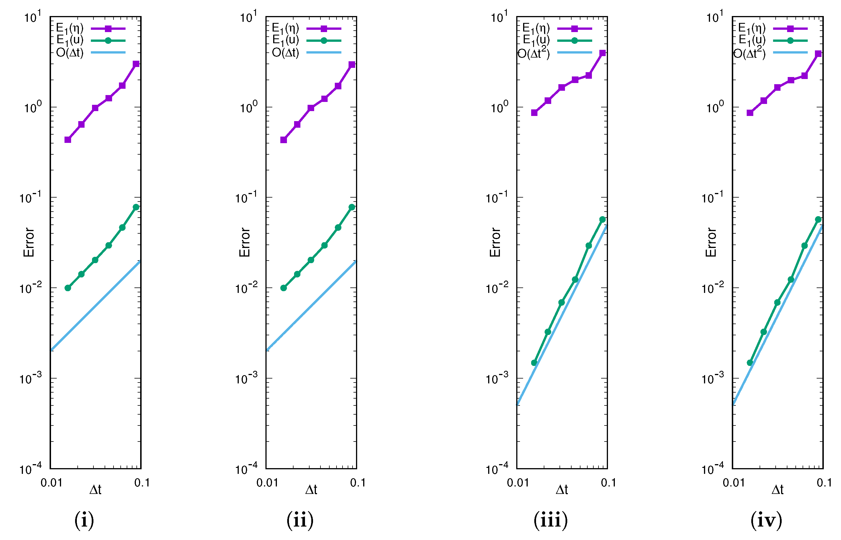
3.1. Experimental Order of Convergence

We solve Examples 1 and 2 below by LG1 and LG2 and compare the experimental orders of convergence (EOCs).

Example 1

($\Gamma ={\Gamma }_{\mathrm{D}}$). In problem (3), we set $\Omega ={(0,1)}^2$, $\Gamma ={\Gamma }_{\mathrm{D}}$ $({\Gamma }_{\mathrm{T}}=\varnothing )$, $T=1$, $g=\rho =\mu =\zeta =1$, and the function ${\eta }^0$, $u^0$, f and F are given so that the exact solution is

$$\begin{array}{cccc}\hfill \varphi (x,t)& =1+\frac{sin\pi x_{1}sin\pi x_2(2+sin\pi t)}{8},\hfill & \hfill u(x,t)& =\frac{sin\pi x_{1}sin\pi x_2(2+sin\pi t)}{3}\left[\begin{array}{c}1\\ 1\end{array}\right].\hfill \end{array}$$

Example 2

($\Gamma ={\overline{\Gamma }}_{\mathrm{D}}\cup {\overline{\Gamma }}_{\mathrm{T}}$). In Example 1, we replace ${\Gamma }_{\mathrm{T}}$ and ${\Gamma }_{\mathrm{D}}$ with ${\Gamma }_{\mathrm{T}}=\{x\in \Gamma ;x_2=0\}$ and ${\Gamma }_{\mathrm{D}}=\Gamma \backslash {\overline{\Gamma }}_{\mathrm{T}}$, respectively.

For a numerical solution $z_h={\left\{z_h^n\right\}}_{n=0}^{N_T}$ and its exact solution $z={\left\{z^n\right\}}_{n=0}^{N_T}$, we introduce notations of errors, $E_i\left(z\right)$, $i=0,1$, defined by

$$\begin{array}{cccc}\hfill E_0\left(z\right) := & \frac{\parallel z_h{-z\parallel }_{{\ell }^{\infty }\left(L^2\right)}}{{\parallel z\parallel }_{{\ell }^{\infty }\left(L^2\right)}},\hfill & \hfill E_1\left(z\right) := & \frac{\parallel \nabla (z_h-z){\parallel }_{{\ell }^{\infty }\left(L^2\right)}}{{\parallel \nabla z\parallel }_{{\ell }^{\infty }\left(L^2\right)}},\hfill \end{array}$$

where ${\parallel ·\parallel }_{{\ell }^{\infty }\left(L^2\right)}$ is a norm given by

$${\parallel z\parallel }_{{\ell }^{\infty }\left(L^2\right)} := max\{\parallel z^n{\parallel }_{L^2(\Omega )};n=0,\dots ,N_T\}.$$

Let N be a division number of each side of the unit square domain $\Omega$ and $h := 1/N$ a representative mesh size. We prepare non-uniform triangulations of $\Omega$, ${\mathcal{T}}_h$, for $N=8,16,32,64,128$ and 256, cf. Figure 3 for $N=32$.

Figure 3. A sample mesh with $N=32$ for Example 1.

Choosing $\Delta t=0.25\sqrt{h}$, we compute the errors, $E_i\left(\eta \right)$ and $E_i\left(u\right)$, $i=0,1$, by LG1 and LG2. Figure 4 and Figure 5 show graphs of the errors of $E_0\left(·\right)$ and $E_1\left(·\right)$, respectively, in logarithmic scale by LG1 for Example 1 (i) and Example 2 (ii), and by LG2 for Example 1 (iii) and Example 2 (iv), and the values of errors and their EOCs are given in Table 1 and Table 2. We observe that LG2 is of second order in time numerically and that the order is higher than that of LG1. Although $E_1\left(\eta \right)$ is not of second order in time, it is natural as Equation (3a) for $\varphi (=\eta +\zeta )$ does not include any diffusion term.

Figure 4. Graphs of errors $E_0\left(\eta \right)$ and $E_0\left(u\right)$ in logarithmic scale by LG1 for Example 1 (i) and Example 2 (ii), and by LG2 for Example 1 (iii) and Example 2 (iv).

Figure 5. Graphs of errors $E_1\left(\eta \right)$ and $E_1\left(u\right)$ in logarithmic scale by LG1 for Example 1 (i) and Example 2 (ii), and by LG2 for Example 1 (iii) and Example 2 (iv).

Table 1. Values of $E_i\left(\eta \right)$ and $E_i\left(u\right)$, $i=0,1$, by schemes LG1 and LG2 for Example 1 ($\Gamma ={\Gamma }_{\mathrm{D}}$).

		LG1
N	$\Delta \mathit{t}$	${\mathit{E}}_0\left(\mathit{\eta }\right)$	EOC	${\mathit{E}}_0\left(\mathit{u}\right)$	EOC
8	$8.84\times {10}^{-2}$	$3.89\times {10}^0$	-	$3.78\times {10}^{-2}$	-
16	$6.25\times {10}^{-2}$	$2.20\times {10}^0$	1.65	$2.28\times {10}^{-2}$	1.45
32	$4.42\times {10}^{-2}$	$1.45\times {10}^0$	1.19	$1.57\times {10}^{-2}$	1.09
64	$3.13\times {10}^{-2}$	$1.01\times {10}^0$	1.05	$1.10\times {10}^{-2}$	1.03
128	$2.21\times {10}^{-2}$	$7.11\times {10}^{-1}$	1.01	$7.77\times {10}^{-3}$	1.00
256	$1.56\times {10}^{-2}$	$5.02\times {10}^{-1}$	1.00	$5.51\times {10}^{-3}$	0.99
		LG1
$\mathit{N}$	$\Delta \mathit{t}$	${\mathit{E}}_{\mathbf{1}}\left(\mathbf{\eta }\right)$	EOC	${\mathit{E}}_{\mathbf{1}}\left(\mathbf{u}\right)$	EOC
8	$8.84\times {10}^{-2}$	$3.00\times {10}^0$	-	$7.78\times {10}^{-2}$	-
16	$6.25\times {10}^{-2}$	$1.73\times {10}^0$	1.59	$4.63\times {10}^{-2}$	1.49
32	$4.42\times {10}^{-2}$	$1.25\times {10}^0$	0.93	$2.95\times {10}^{-2}$	1.31
64	$3.13\times {10}^{-2}$	$9.78\times {10}^{-1}$	0.71	$2.04\times {10}^{-2}$	1.06
128	$2.21\times {10}^{-2}$	$6.42\times {10}^{-1}$	1.22	$1.42\times {10}^{-2}$	1.04
256	$1.56\times {10}^{-2}$	$4.35\times {10}^{-1}$	1.12	$1.00\times {10}^{-2}$	1.01
		LG2
$\mathit{N}$	$\Delta \mathit{t}$	${\mathit{E}}_{\mathbf{0}}\left(\mathbf{\eta }\right)$	EOC	${\mathit{E}}_{\mathbf{0}}\left(\mathbf{u}\right)$	EOC
8	$8.84\times {10}^{-2}$	$6.81\times {10}^{-1}$	-	$1.71\times {10}^{-2}$	-
16	$6.25\times {10}^{-2}$	$1.96\times {10}^{-1}$	3.60	$7.03\times {10}^{-3}$	2.57
32	$4.42\times {10}^{-2}$	$8.53\times {10}^{-2}$	2.40	$3.32\times {10}^{-3}$	2.16
64	$3.13\times {10}^{-2}$	$3.82\times {10}^{-2}$	2.32	$1.64\times {10}^{-3}$	2.04
128	$2.21\times {10}^{-2}$	$1.87\times {10}^{-2}$	2.05	$8.20\times {10}^{-4}$	1.99
256	$1.56\times {10}^{-2}$	$9.46\times {10}^{-3}$	1.97	$4.17\times {10}^{-4}$	1.95
		LG2
$\mathit{N}$	$\Delta \mathit{t}$	${\mathit{E}}_{\mathbf{1}}\left(\mathbf{\eta }\right)$	EOC	${\mathit{E}}_{\mathbf{1}}\left(\mathbf{u}\right)$	EOC
8	$8.84\times {10}^{-2}$	$3.97\times {10}^0$	-	$5.68\times {10}^{-2}$	-
16	$6.25\times {10}^{-2}$	$2.24\times {10}^0$	1.65	$2.90\times {10}^{-2}$	1.94
32	$4.42\times {10}^{-2}$	$2.00\times {10}^0$	0.33	$1.20\times {10}^{-2}$	2.54
64	$3.13\times {10}^{-2}$	$1.64\times {10}^0$	0.57	$6.72\times {10}^{-3}$	1.67
128	$2.21\times {10}^{-2}$	$1.17\times {10}^0$	0.97	$3.23\times {10}^{-3}$	2.11
256	$1.56\times {10}^{-2}$	$8.64\times {10}^{-1}$	0.88	$1.47\times {10}^{-3}$	2.28

Table 2. Values of $E_i\left(\eta \right)$ and $E_i\left(u\right)$, $i=0,1$, by schemes LG1 and LG2 for Example 2 ($\Gamma ={\overline{\Gamma }}_{\mathrm{D}}\cup {\overline{\Gamma }}_{\mathrm{T}}$).

		LG1
N	$\Delta \mathit{t}$	${\mathit{E}}_0\left(\mathit{\eta }\right)$	EOC	${\mathit{E}}_0\left(\mathit{u}\right)$	EOC
8	$8.84\times {10}^{-2}$	$3.88\times {10}^0$	-	$3.86\times {10}^{-2}$	-
16	$6.25\times {10}^{-2}$	$2.19\times {10}^0$	1.65	$2.33\times {10}^{-2}$	1.46
32	$4.42\times {10}^{-2}$	$1.45\times {10}^0$	1.19	$1.58\times {10}^{-2}$	1.11
64	$3.13\times {10}^{-2}$	$1.01\times {10}^0$	1.05	$1.11\times {10}^{-2}$	1.03
128	$2.21\times {10}^{-2}$	$7.09\times {10}^{-1}$	1.01	$7.82\times {10}^{-3}$	1.01
256	$1.56\times {10}^{-2}$	$5.01\times {10}^{-1}$	1.00	$5.53\times {10}^{-3}$	1.00
		LG1
$\mathit{N}$	$\Delta \mathit{t}$	${\mathit{E}}_{\mathbf{1}}\left(\mathbf{\eta }\right)$	EOC	${\mathit{E}}_{\mathbf{1}}\left(\mathbf{u}\right)$	EOC
8	$8.84\times {10}^{-2}$	$2.95\times {10}^0$	-	$7.80\times {10}^{-2}$	-
16	$6.25\times {10}^{-2}$	$1.71\times {10}^0$	1.57	$4.64\times {10}^{-2}$	1.50
32	$4.42\times {10}^{-2}$	$1.24\times {10}^0$	0.94	$2.95\times {10}^{-2}$	1.31
64	$3.13\times {10}^{-2}$	$9.78\times {10}^{-1}$	0.67	$2.03\times {10}^{-2}$	1.07
128	$2.21\times {10}^{-2}$	$6.42\times {10}^{-1}$	1.21	$1.41\times {10}^{-2}$	1.04
256	$1.56\times {10}^{-2}$	$4.34\times {10}^{-1}$	1.13	$9.96\times {10}^{-3}$	1.01
		LG2
$\mathit{N}$	$\Delta \mathit{t}$	${\mathit{E}}_{\mathbf{0}}\left(\mathbf{\eta }\right)$	EOC	${\mathit{E}}_{\mathbf{0}}\left(\mathbf{u}\right)$	EOC
8	$8.84\times {10}^{-2}$	$6.70\times {10}^{-1}$	-	$1.75\times {10}^{-2}$	-
16	$6.25\times {10}^{-2}$	$1.95\times {10}^{-1}$	3.56	$7.23\times {10}^{-3}$	2.55
32	$4.42\times {10}^{-2}$	$8.58\times {10}^{-2}$	2.37	$3.37\times {10}^{-3}$	2.20
64	$3.13\times {10}^{-2}$	$3.97\times {10}^{-2}$	2.22	$1.67\times {10}^{-3}$	2.03
128	$2.21\times {10}^{-2}$	$1.87\times {10}^{-2}$	2.17	$8.37\times {10}^{-4}$	2.00
256	$1.56\times {10}^{-2}$	$9.54\times {10}^{-3}$	1.94	$4.25\times {10}^{-4}$	1.96
		LG2
$\mathit{N}$	$\Delta \mathit{t}$	${\mathit{E}}_{\mathbf{1}}\left(\mathbf{\eta }\right)$	EOC	${\mathit{E}}_{\mathbf{1}}\left(\mathbf{u}\right)$	EOC
8	$8.84\times {10}^{-2}$	$3.89\times {10}^0$	-	$5.70\times {10}^{-2}$	-
16	$6.25\times {10}^{-2}$	$2.21\times {10}^0$	1.63	$2.93\times {10}^{-2}$	1.92
32	$4.42\times {10}^{-2}$	$1.98\times {10}^0$	0.32	$1.24\times {10}^{-2}$	2.49
64	$3.13\times {10}^{-2}$	$1.65\times {10}^0$	0.54	$6.90\times {10}^{-3}$	1.69
128	$2.21\times {10}^{-2}$	$1.17\times {10}^0$	0.97	$3.26\times {10}^{-3}$	2.16
256	$1.56\times {10}^{-2}$	$8.62\times {10}^{-1}$	0.89	$1.48\times {10}^{-3}$	2.27

Remark 5.

Lagrange–Galerkin schemes are basically CFL-free, and our scheme also has this property. In fact, the CFL number in this computation is $U\Delta t/h=1/\left(4\sqrt{h}\right)=4$ for $N=256$ as the maximum velocity U is 1 and the $\Delta t$ is chosen as $\Delta t=0.25\sqrt{h}$.

3.2. Effect of the TBC

We consider the following example to see the effect of the TBC.

Example 3.

In problem (3), we set $\Omega ={(0,10)}^2$, $T=100$, $g=\rho =\mu =\zeta =1$, $(f,F)=(0,0)$, ${\eta }^0={cexp(-100|x-p|}^2)$, $c={10}^{-3}$, $p={(5,5)}^{\top }$, and $u^0=0$. We consider five cases of ${\Gamma }_{\mathrm{T}}$,

(a)

${\Gamma }_{\mathrm{T}}=\varnothing$, i.e., $\Gamma ={\Gamma }_{\mathrm{D}}$,

(b)

${\Gamma }_{\mathrm{T}}=\{x\in \Gamma ;x_2=0\}$ (bottom), ${\Gamma }_{\mathrm{D}}=\Gamma \backslash {\overline{\Gamma }}_{\mathrm{T}}$,

(c)

${\Gamma }_{\mathrm{T}}=\{x\in \Gamma ;x_1=10,x_2=0\}$ (right and bottom), ${\Gamma }_{\mathrm{D}}=\Gamma \backslash {\overline{\Gamma }}_{\mathrm{T}}$,

(d)

${\Gamma }_{\mathrm{T}}=\{x\in \Gamma ;x_1=10,x_2=0,10\}$ (right, bottom and top), ${\Gamma }_{\mathrm{D}}=\Gamma \backslash {\overline{\Gamma }}_{\mathrm{T}}$,

(e)

${\Gamma }_{\mathrm{T}}=\Gamma$.

We solve Example 3 by LG2. Figure 6 shows the color contours of ${\eta }_h^n$ for $t=25k$, $k=0,\dots ,4$, cf. (i)–(v), for the five cases, (a)–(e). We can see the effect of the boundary conditions; the artificial reflection is observed and removed significantly when the wave touches the Dirichlet $\left({\Gamma }_{\mathrm{D}}\right)$ and the transmission $\left({\Gamma }_{\mathrm{T}}\right)$ boundaries, respectively. Thus, LG2 works well for the SWEs with and without the TBC in the simple square domain.

Figure 6. Color contours of ${\eta }_h^n$ by LG2 with and without the TBC for the five cases, (a–e), in Example 3.

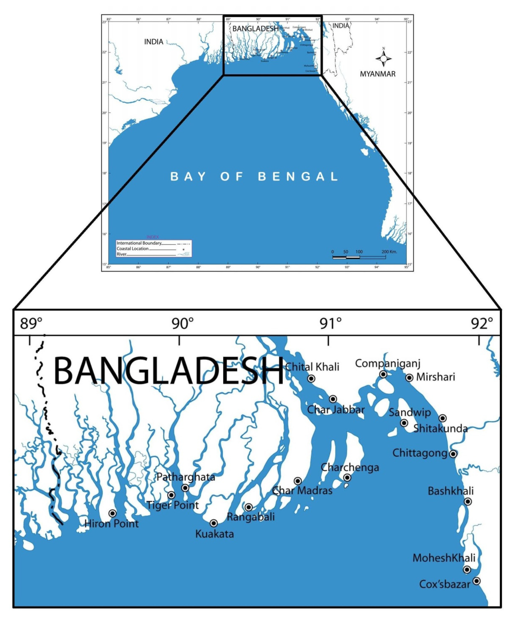
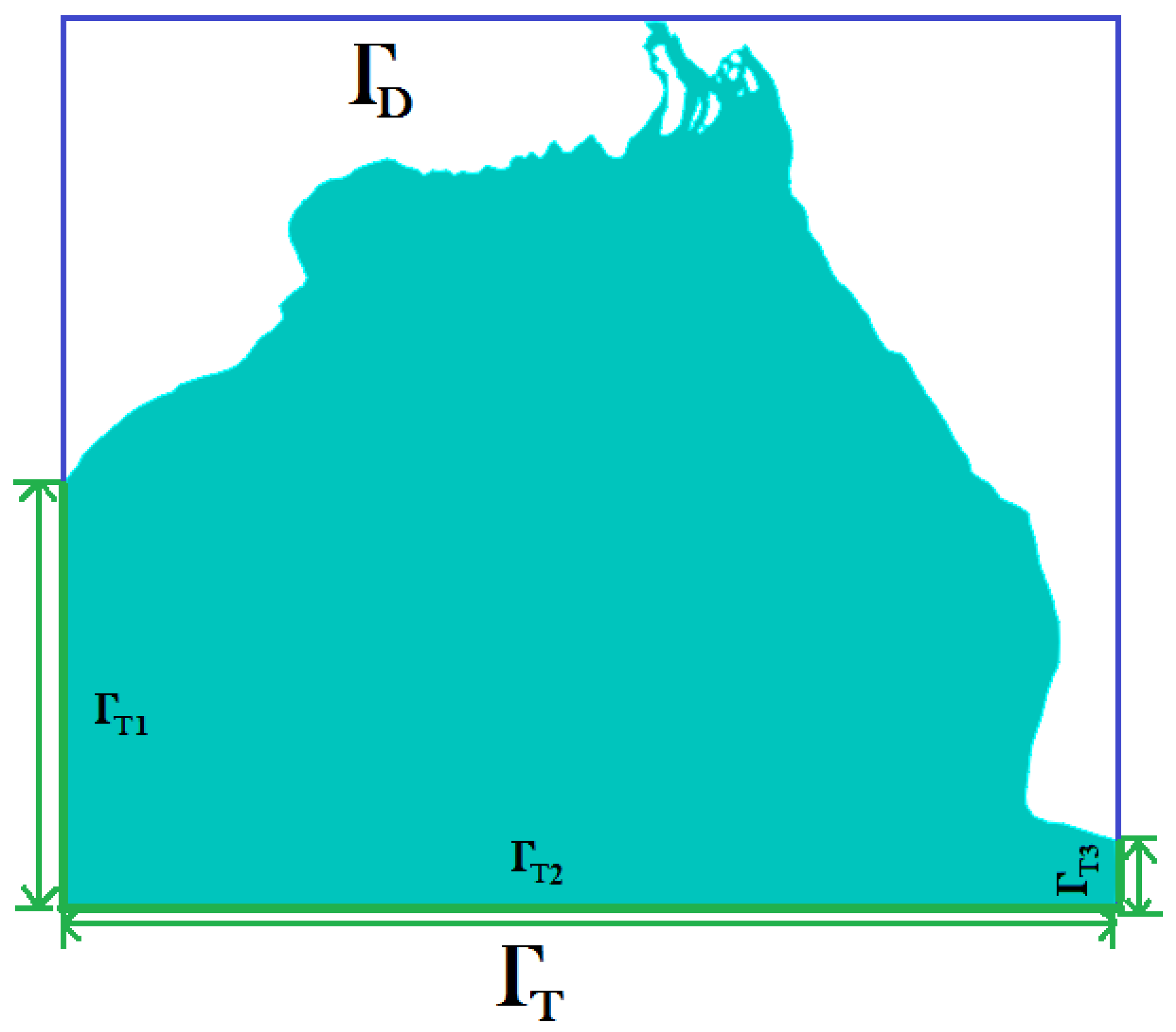
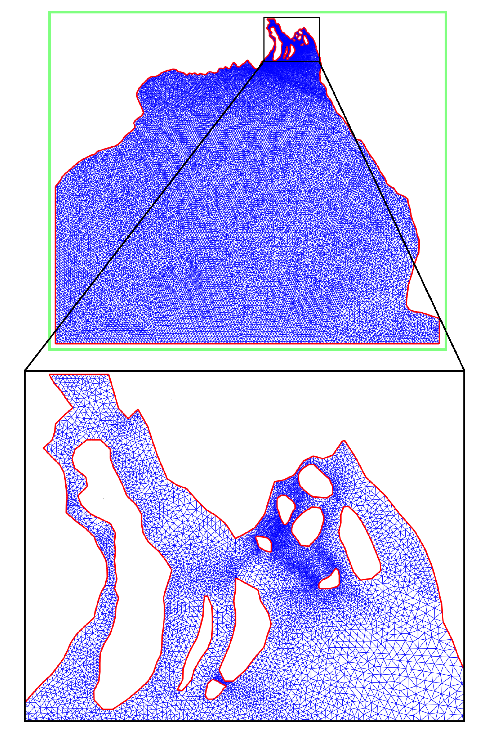
4. Application to the Bay of Bengal

In this section, we apply LG2, i.e., scheme (5) discussed in Section 2.2, to a computational domain of the Bay of Bengal region, cf. Figure 7, which is an approximate domain of the original, cf. Figure 1. All the computations are performed via FreeFem++ [50].

Figure 7. The domain for the Bay of Bengal region with the information of boundaries, ${\Gamma }_{\mathrm{D}}$ and ${\Gamma }_{\mathrm{T}}(={\Gamma }_{\mathrm{T}1}\cup {\Gamma }_{\mathrm{T}2}\cup {\Gamma }_{\mathrm{T}3})$ used in Example 4.

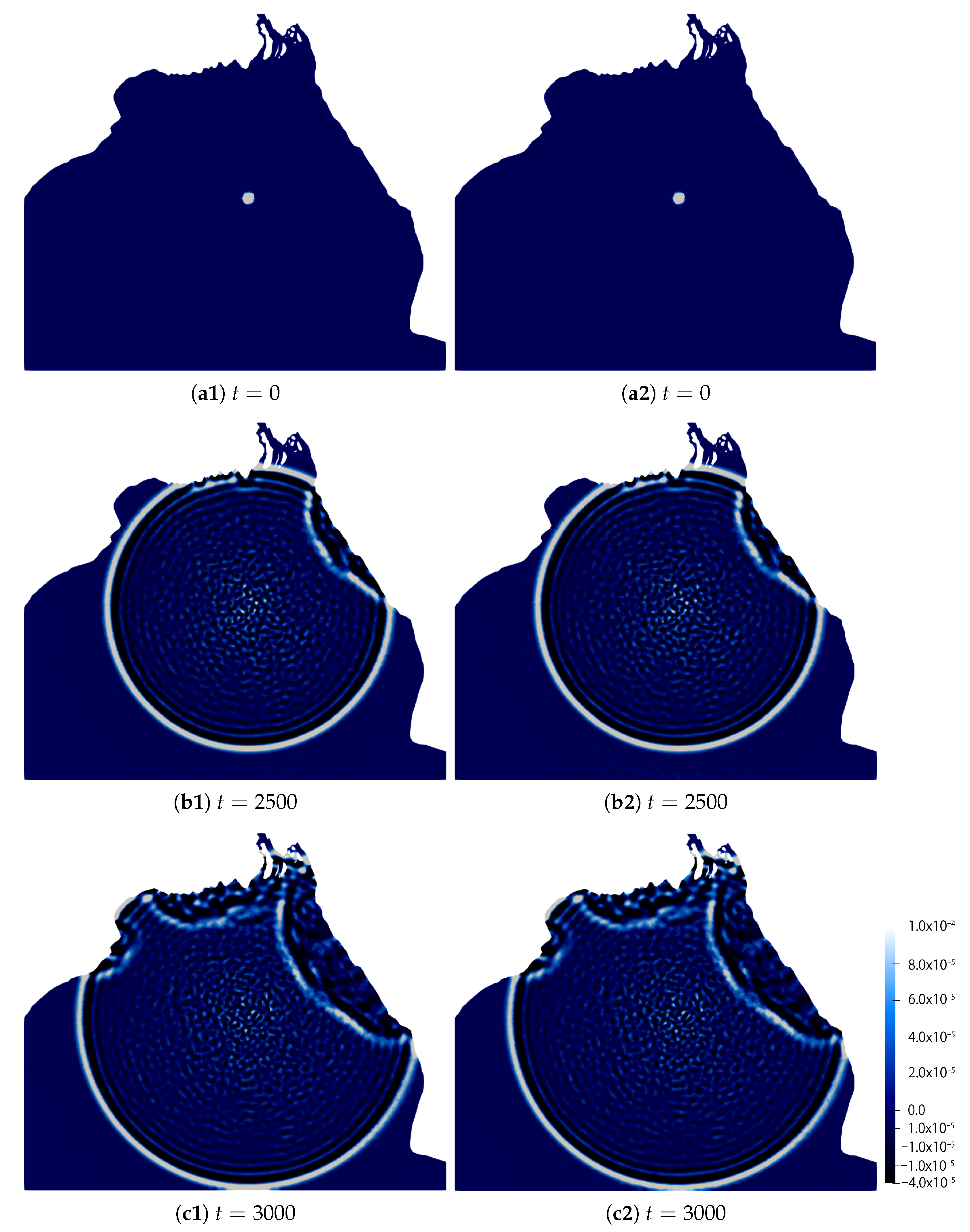
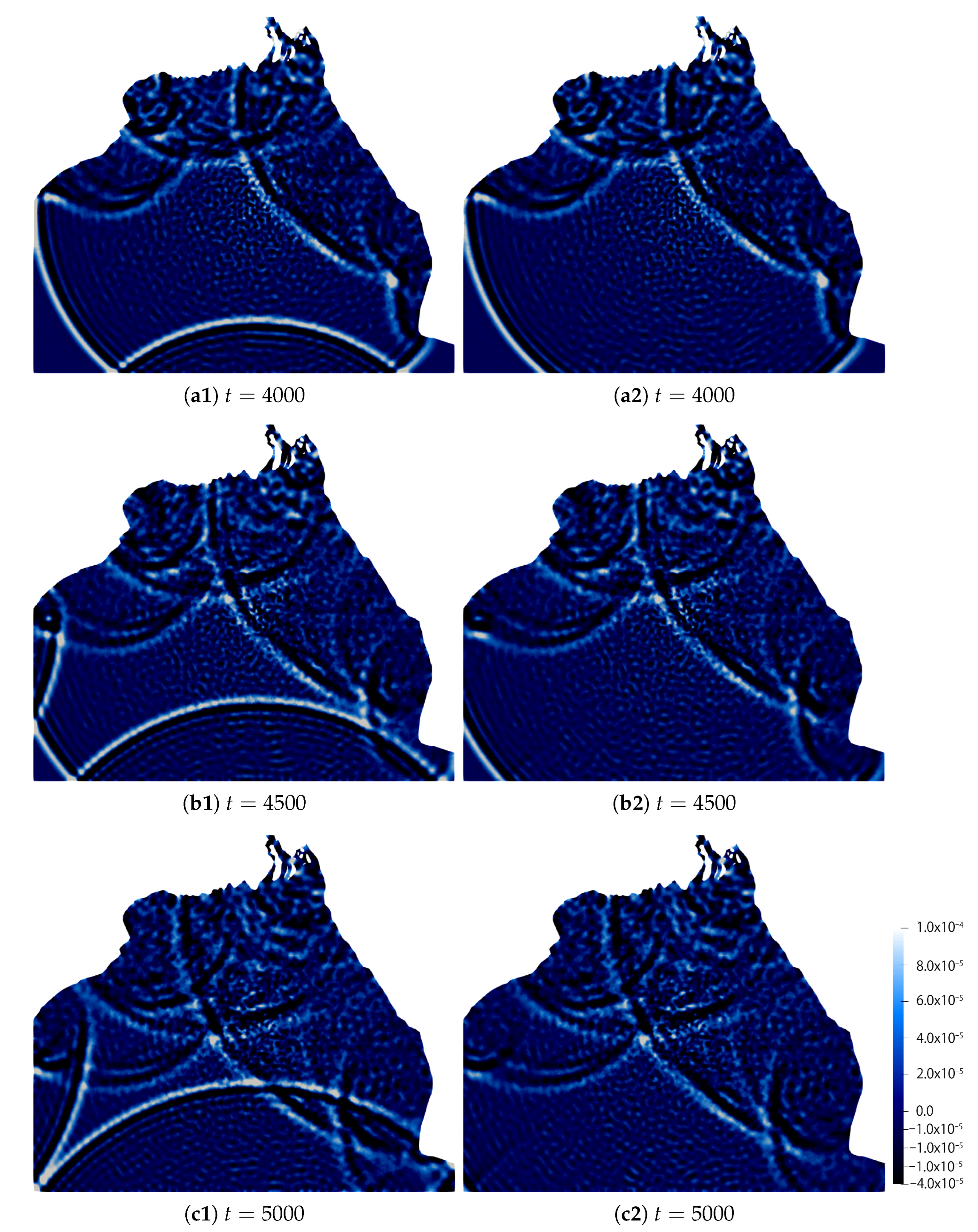
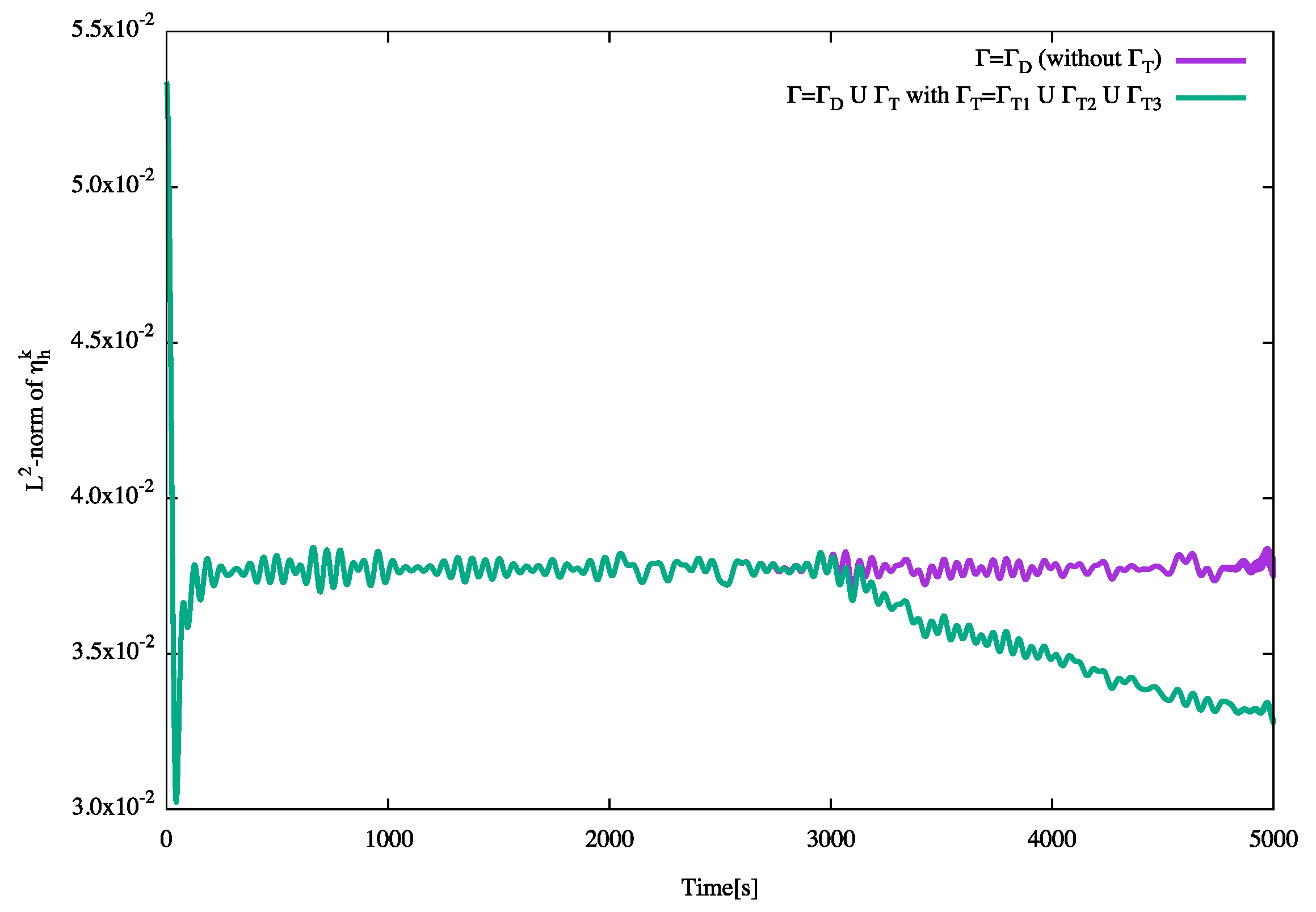
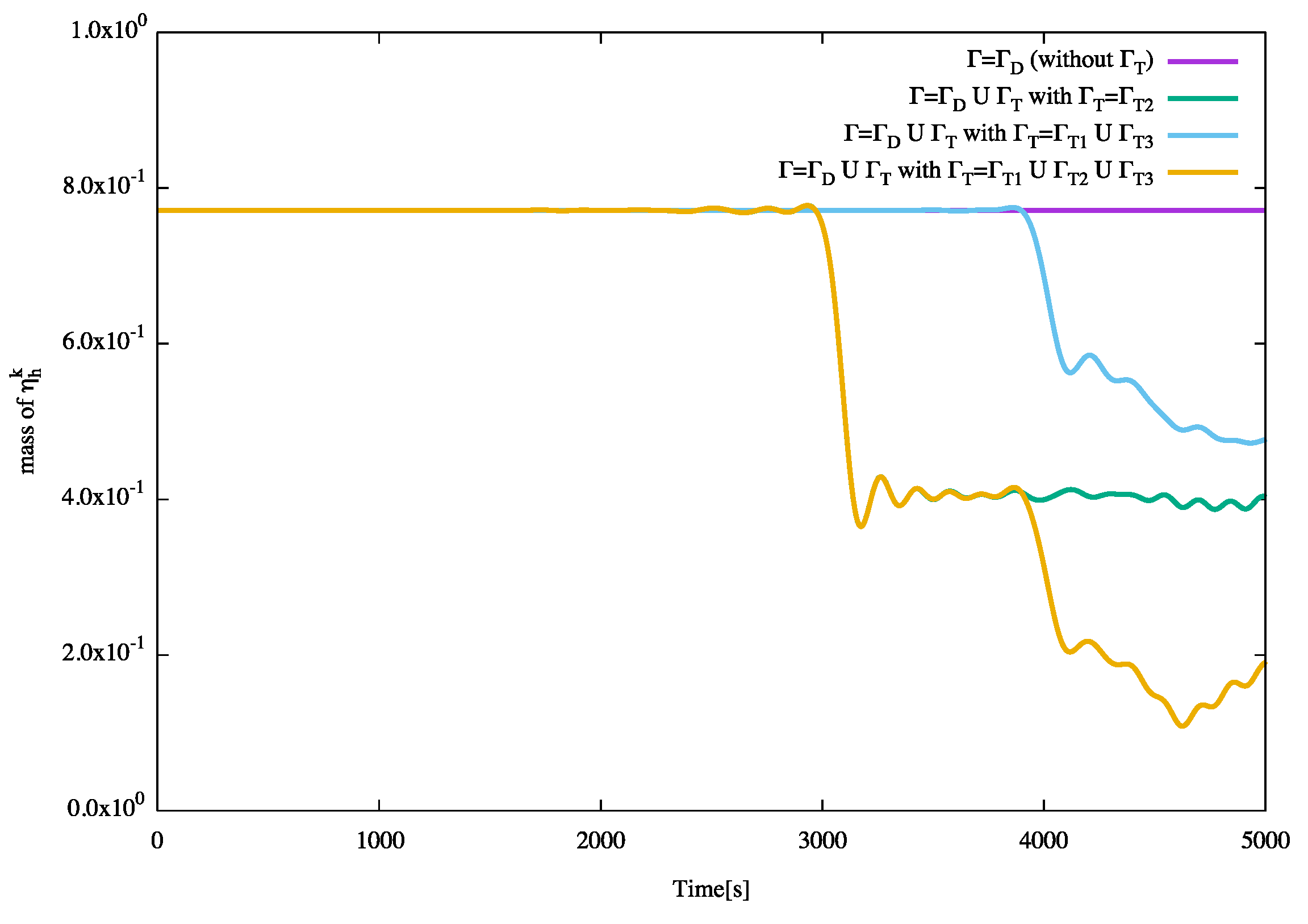
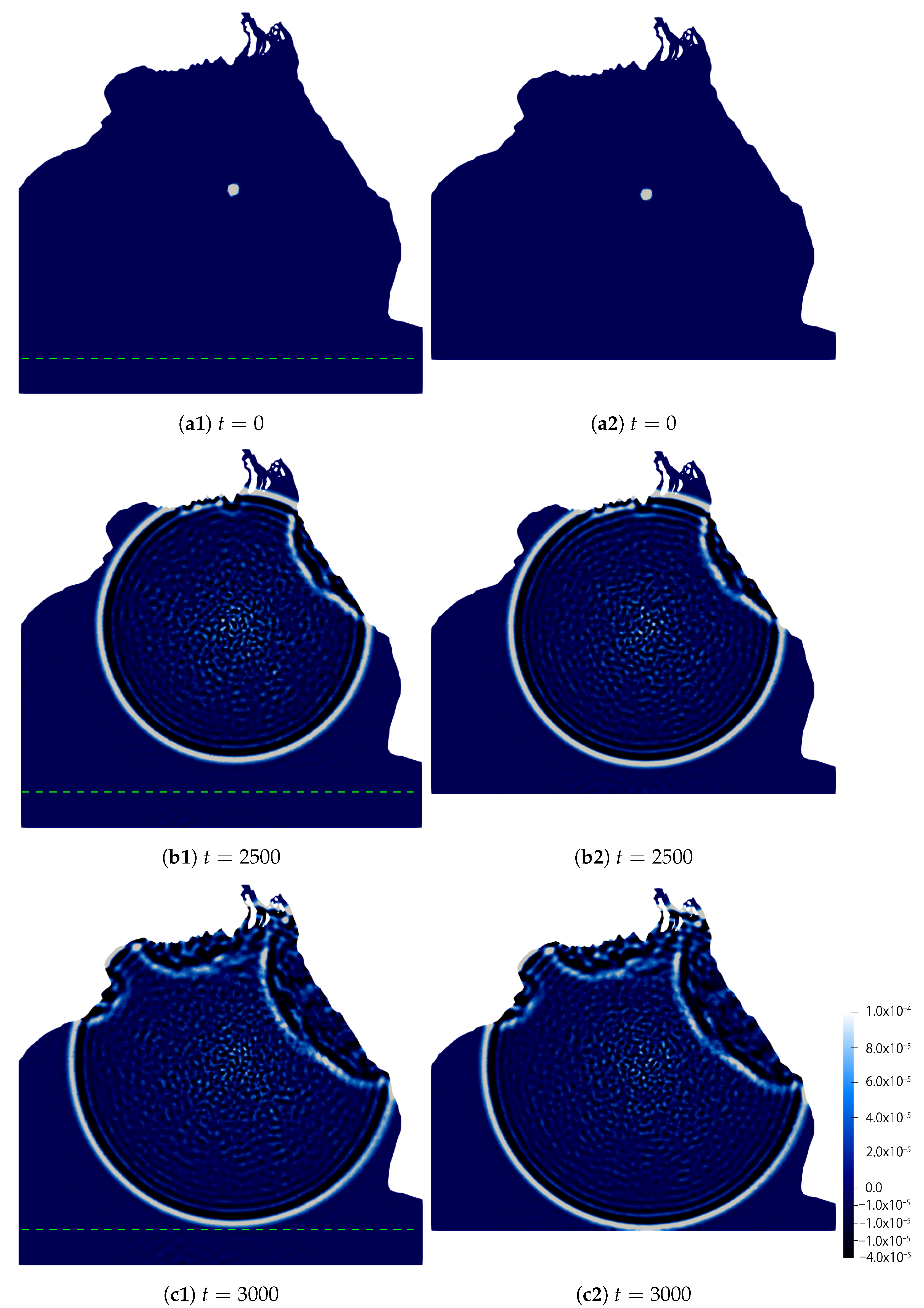
4.1. Numerical Simulation with and without the TBC

We set the following example.

Example 4.

Let Ω be the domain shown in Figure 7. The domain is considered from 0 to $1051.4\left[\mathrm{km}\right]$ in the horizontal direction and 0 to $889.59\left[\mathrm{km}\right]$ in the vertical direction. We employ two boundary conditions, the Dirichlet boundary condition on ${\Gamma }_{\mathrm{D}}$ and the TBC on ${\Gamma }_{\mathrm{T}}$, cf. Figure 7. We set ${\Gamma }_{\mathrm{D}}$ on the coastal and island boundaries and ${\Gamma }_{\mathrm{T}}$ on the artificial boundaries for the open sea. As shown in Figure 7, there are three artificial boundaries on the open sea, i.e., ${\Gamma }_{\mathrm{T}}={\Gamma }_{\mathrm{T}1}\cup {\Gamma }_{\mathrm{T}2}\cup {\Gamma }_{\mathrm{T}3}$. In problem (3), we set $T=5000\left[\mathrm{s}\right]$, $\zeta =2\left[\mathrm{km}\right]$, ${\eta }^0\left(x\right)=c_1{exp(-0.04|x-p|}^2)\left[\mathrm{km}\right]$, $c_1=0.01[-]$, $p={(559.56,430.02)}^{\top }$, $u^0=0$, $\mu =1[\mathrm{Pa}·\mathrm{s}]$, $\rho ={10}^{12}[\mathrm{kg}/{\mathrm{km}}^3]$, $g=9.8\times {10}^{-3}[\mathrm{km}/{\mathrm{s}}^2]$ and $(f,F)=(0,0)$.

We prepare a triangular mesh of the domain as shown in Figure 8, where the numbers of elements and nodal points are $\text{60,619}$ and $\text{31,120}$, respectively. Then, a numerical simulation is done by LG2 with $\Delta t=0.2$ [$\mathrm{s}$]. The results at $t=0,2500,3000,4000,4500$ and 5000 [$\mathrm{s}$] are presented in Figure 9 and Figure 10. In the figures, for comparison to see the effect of the TBC, we compute Example 4 by replacing ${\Gamma }_{\mathrm{T}}$ with ${\Gamma }_{\mathrm{D}}$ and put it on the left. From Figure 9, we can see that a circular wave is created at around the point p, that it propagates towards the boundary over time, that reflections are found when the wave touches ${\Gamma }_{\mathrm{D}}$, and that the results with $\Gamma ={\Gamma }_{\mathrm{D}}$ (left) and $\Gamma ={\Gamma }_{\mathrm{D}}\cup {\Gamma }_{\mathrm{T}}$ (right) are similar. From Figure 10, we can observe that artificial reflections on the open sea boundaries are significantly removed when the wave touches ${\Gamma }_{\mathrm{T}}$, cf. the right figures. Thus, LG2 works well for a simple (square) domain and this complex domain, the Bay of Bengal region, which is non-convex and includes islands.

Figure 8. The mesh for the Bay of Bengal region used for Example 4.

Figure 9. Contour plot of ${\eta }_h^n$ by LG2 with $\Gamma ={\Gamma }_{\mathrm{D}}$ (left) and $\Gamma ={\Gamma }_{\mathrm{D}}\cup {\Gamma }_{\mathrm{T}}$ (right) on the Bay of Bengal for $t=0,2500$ and $3000$.

Figure 10. Contour plot of ${\eta }_h^n$ by LG2 with $\Gamma ={\Gamma }_{\mathrm{D}}$ (left) and $\Gamma ={\overline{\Gamma }}_{\mathrm{D}}\cup {\overline{\Gamma }}_{\mathrm{T}}$ (right) on the Bay of Bengal for $t=4000,4500$ and $5000$.

For any (smooth) solution to problem (3), we define the total energy $\mathcal{E}\left(t\right)$ by

$$\begin{array}{c}\hfill \mathcal{E}\left(t\right) := {\mathcal{E}}_1\left(t\right)+{\mathcal{E}}_2\left(t\right) := {\int }_{\Omega }\frac{\rho }{2}\varphi {\left|u\right|}^{2}dx+{\int }_{\Omega }\frac{{\rho g\left|\eta \right|}^2}{2}dx,\end{array}$$

(6)

where ${\mathcal{E}}_1\left(t\right)$ is the kinetic energy, and ${\mathcal{E}}_2\left(t\right)$ is the potential energy. Then, it is worthy to note that the following energy estimate holds, cf. ([9] Corollary 3.3-(i)),

$$\begin{array}{cc}\hfill \frac{d}{dt}\mathcal{E}\left(t\right)& =-\frac{\rho }{2}{\int }_{{\Gamma }_{\mathrm{T}}}\varphi {\left|u\right|}^{2}u·nds-\rho g{\int }_{{\Gamma }_{\mathrm{T}}}\varphi \eta u·nds\hfill \\ \hfill & +2\mu {\int }_{{\Gamma }_{\mathrm{T}}}\varphi \left[D\left(u\right)n\right]·uds-2\mu {\int }_{\Omega }\varphi {\left|D\left(u\right)\right|}^{2}dx.\hfill \end{array}$$

(7)

Here, focusing on ${\mathcal{E}}_2\left(t\right)$ $(=\frac{1}{2}{\int }_{\Omega }\rho g|\eta {|}^{2}dx)$ and the mass of $\eta$, i.e., ${\int }_{\Omega }\eta dx$, we present the values of the $L^2(\Omega )$-norm of ${\eta }_h^n$, i.e, $\parallel {\eta }_h^n{\parallel }_{L^2(\Omega )}$, and the mass of ${\eta }_h^n$, i.e., ${\int }_{\Omega }{\eta }_h^{n}dx$, in Figure 11 and Figure 12, respectively. In principle, we can say that the TBC works well numerically if $\parallel {\eta }_h^n{\parallel }_{L^2(\Omega )}$ and ${\int }_{\Omega }{\eta }_h^{n}dx$ decrease around the time that the wave touches the transmission boundaries. Figure 11 shows graphs of $\parallel {\eta }_h^n{\parallel }_{L^2(\Omega )}$ for the two cases, with and without the transmission boundaries, i.e., $\Gamma ={\Gamma }_{\mathrm{D}}\cup {\Gamma }_{\mathrm{T}}$ and $\Gamma ={\Gamma }_{\mathrm{D}}({\Gamma }_{\mathrm{T}}=\varnothing )$, respectively. Figure 12 shows the graphs of ${\int }_{\Omega }{\eta }_h^{n}dx$ for the four cases of (transmission) boundaries, (i) no transmission boundary, i.e., ${\Gamma }_{\mathrm{T}}=\varnothing$, (ii) one transmission boundary, i.e., ${\Gamma }_{\mathrm{T}}={\Gamma }_{\mathrm{T}2}$, (iii) two transmission boundaries, i.e., ${\Gamma }_{\mathrm{T}}={\Gamma }_{\mathrm{T}1}\cup {\Gamma }_{\mathrm{T}3}$, and (iv) three transmission boundaries, i.e., ${\Gamma }_{\mathrm{T}}={\Gamma }_{\mathrm{T}1}\cup {\Gamma }_{\mathrm{T}2}\cup {\Gamma }_{\mathrm{T}3}$. From Figure 11 and Figure 12, we can see that there are decreasing phenomena of the value of $L^2(\Omega )$-norm as well as the value of the mass when the TBC is imposed. From Figure 9, we can see that the wave touches the transmission boundary ${\Gamma }_{\mathrm{T}2}$ at time around $t=3000$ [s]; that is why, the mass of ${\eta }_h^n$ decreases drastically from around 3000 [s] to 3200 [s], cf. Figure 12 (yellow and green lines). Again, the mass started to decrease between the period from around 4000 [s] to 4500 [s], cf. Figure 12, since the wave reached the transmission boundary ${\Gamma }_{\mathrm{T}1}$ and ${\Gamma }_{\mathrm{T}3}$, cf. Figure 10.

Figure 11. Graphs of $\parallel {\eta }_h^n{\parallel }_{L^2(\Omega )}$ with respect to time $(t=t^n)$ for Example 4 with ${\Gamma }_{\mathrm{T}}$$(\Gamma ={\Gamma }_{\mathrm{D}}\cup {\Gamma }_{\mathrm{T}})$ and without ${\Gamma }_{\mathrm{T}}$$(\Gamma ={\Gamma }_{\mathrm{D}})$.

Figure 12. Graphs of the mass of ${\eta }_h^n$ with respect to time $(t=t^n)$ for Example 4 with the following four settings; no transmission boundary, i.e., ${\Gamma }_{\mathrm{T}}=\varnothing$ (purple), one transmission boundary, i.e., ${\Gamma }_{\mathrm{T}}={\Gamma }_{\mathrm{T}2}$ (green), two transmission boundaries, i.e., ${\Gamma }_{\mathrm{T}}={\Gamma }_{\mathrm{T}1}\cup {\Gamma }_{\mathrm{T}3}$ (blue), and three transmission boundaries, i.e., ${\Gamma }_{\mathrm{T}}={\Gamma }_{\mathrm{T}1}\cup {\Gamma }_{\mathrm{T}2}\cup {\Gamma }_{\mathrm{T}3}$ (yellow).

Remark 6.

We recall the results in [9] and mention the advantage of the TBC Equation (3e) on the stability under the assumption $\varphi >0$ on ${\Gamma }_{\mathrm{T}}\times [0,T]$.

(i)

The last term in the RHS of (7) is obviously non-positive. From the TBC Equation (3e), i.e., $\varphi u=c_0\sqrt{g\zeta }\eta n$, we observe that the second term in the RHS of Equation (7) is non-positive:

$$-\rho g{\int }_{{\Gamma }_{\mathrm{T}}}\varphi \eta u·nds=-\rho g{\int }_{{\Gamma }_{\mathrm{T}}}{c}_0\sqrt{g\zeta }{\eta }^{2}ds\le 0.$$

Since it is numerically observed in [9] that the second term is dominant from the viewpoint of the energy $\mathcal{E}\left(t\right)$, cf. ([9] (Remark 3.5)), we can expect that this non-positivity derived from the TBC Equation (3e) improves the stability of the SWEs Equation (3).

(ii)

Let us additionally introduce a theorem ([9] (Theorem 3.4)). Suppose that there exists $\alpha \in (0,1)$ such that

$$\begin{array}{cc}\hfill \eta (x,t)& \ge -\alpha \zeta \left(x\right)(x\in {\overline{\Gamma }}_{\mathrm{T}},t\in [0,T]),\hfill \\ \hfill 0& <c_0\le \sqrt{2/\alpha }(1-\alpha ).\hfill \end{array}$$

(8)

Then, the summation of the first and second terms in the RHS of Equation (7) is non-positive, i.e.,

$$\begin{array}{c}\hfill -\frac{\rho }{2}{\int }_{{\Gamma }_{\mathrm{T}}}\varphi {\left|u\right|}^{2}u·nds-\rho g{\int }_{{\Gamma }_{\mathrm{T}}}\varphi \eta u·nds\le 0,\end{array}$$

in particular,

$$\begin{array}{cc}\hfill \frac{d}{dt}\mathcal{E}\left(t\right)& \le 2\mu {\int }_{{\Gamma }_{\mathrm{T}}}\varphi \left[D\left(u\right)n\right]·uds.\hfill \end{array}$$

(iii)

As mentioned in ([9] (Remark 3.6)), the condition (8) is not strict in the practical computation, where α and $c_0$ are chosen typically as, e.g., $\alpha =0.01$ and $c_0=0.9$. These satisfy condition (8) since $\sqrt{2/\alpha }(1-\alpha )\approx 14$.

(iv)

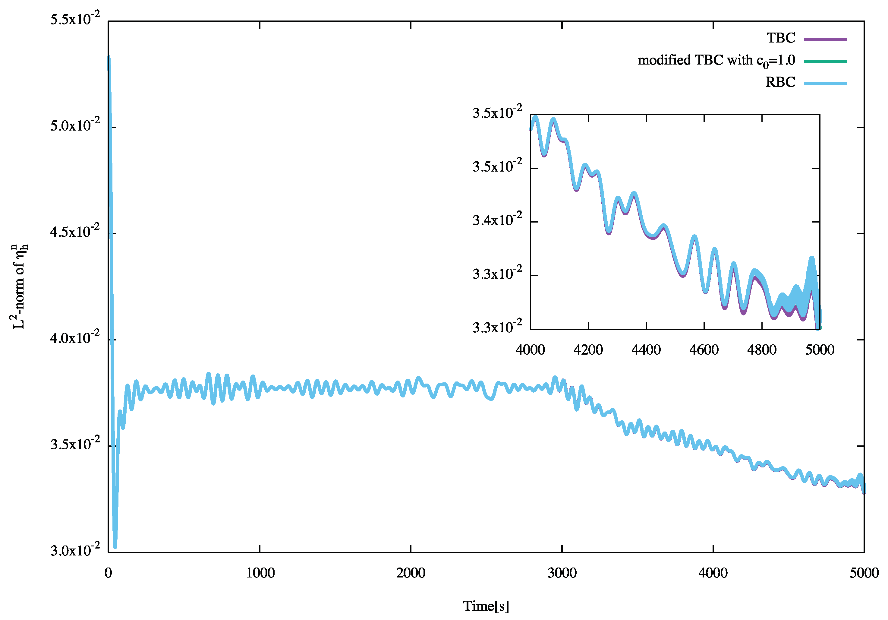
We have compared our results by the TBC ($c_0=0.9$) and a modified TBC ($c_0=1$) with those by the RBC:

$$\begin{array}{c}\hfill u=\sqrt{g/\zeta }\eta non{\Gamma }_{\mathrm{T}}\times (0,T).\end{array}$$

(9)

The results by the three boundary conditions are not significantly different as presented in Appendix B. We note that condition (9) is the well-known RBC, cf., e.g., [8], and that the modified TBC is obtained by replacing ζ with ${\varphi }^2/\zeta$ in Equation (9), where the relation $\zeta \approx {\varphi }^2/\zeta \approx \varphi$ holds if $\left|\eta \right|\ll \zeta$ is satisfied.

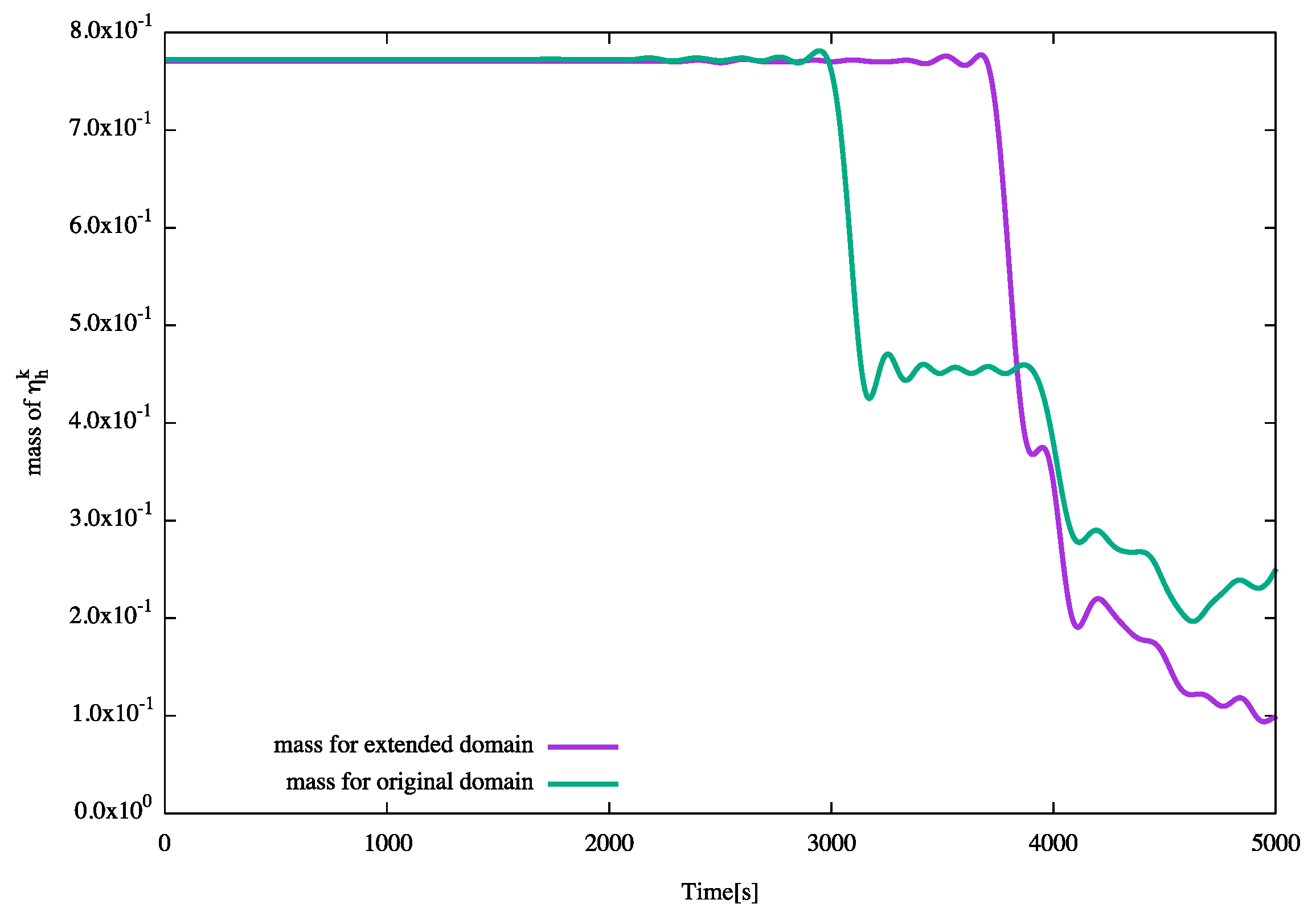
4.2. Effect of Position of a Transmission Boundary

We consider Example 4 again to see the effect of the TBC with an extension of the domain ($\Omega$), where the size of the domain in the vertical direction is extended from $889.59\left[\mathrm{km}\right]$ to $989.59\left[\mathrm{km}\right]$, i.e., $100\left[\mathrm{km}\right]$ extension. We employ the same boundary conditions on $\Gamma ={\Gamma }_{\mathrm{D}}\cup {\Gamma }_{\mathrm{T}}$ for both original and extended domains, where ${\Gamma }_{\mathrm{T}}={\Gamma }_{\mathrm{T}1}\cup {\Gamma }_{\mathrm{T}2}\cup {\Gamma }_{\mathrm{T}3}$. We compare the numerical results for the extended domain with the ones for the original domain, cf. Figure 13 and Figure 14, where the left and right figures show the results for the extended and original domains, respectively. It is observed that there is no significant effect of the vertical position of the bottom transmission boundary ${\Gamma }_{\mathrm{T}2}$. We also computed the mass of $\eta$ for both domains, cf. Figure 15. From Figure 15, we can see that the mass of ${\eta }_h^k$ started to decrease at time $t=3000$ for the original domain, cf. Figure 13c2, while the mass of ${\eta }_h^k$ started to decrease at time $t=4000$ for the extended domain, cf. Figure 14b1, because the wave touches the boundary ${\Gamma }_{\mathrm{T}2}$ at these times ($t=3000$ and $t=4000$) for the original and extended domains, respectively. A similar decreasing property of mass of ${\eta }_h^k$ can be observed from Figure 15 when the wave touches the transmission boundaries. The results confirm that the TBC works well numerically and that we can choose the vertical position of the bottom transmission boundary ${\Gamma }_{\mathrm{T}2}$ without significant effect.

Figure 13. Contour plot of ${\eta }_h^n$ by LG2 with $\Gamma ={\overline{\Gamma }}_{\mathrm{D}}\cup {\overline{\Gamma }}_{\mathrm{T}}$ for the extended domain (left) and for the original domain (right) on the Bay of Bengal for $t=0,2500$ and $3000$. The green dotted lines in the left figures indicate the position of the bottom boundary of the original domain.

Figure 14. Contour plot of ${\eta }_h^n$ by LG2 with $\Gamma ={\overline{\Gamma }}_{\mathrm{D}}\cup {\overline{\Gamma }}_{\mathrm{T}}$ for the extended domain (left) and for the original domain (right) on the Bay of Bengal for $t=3500,4000$ and $5000$.

Figure 15. Graphs of the mass of ${\eta }_h^n$ for the extended and original domain with a TBC.

5. Conclusions

We have presented a two-step Lagrange–Galerkin scheme for the shallow water equations with a TBC. For the scheme, the EOCs have been computed (cf. Examples 1 and 2 in Section 3.1) and the second-order accuracy in time has been confirmed. From numerical experiments on a simple square domain (cf. Example 3 in Section 3.2), it has been observed that the effect of the TBC works well. Our scheme has been applied to a realistic domain, the Bay of Bengal, and numerical experiments have been performed for two different types of boundary conditions, i.e., with and without the TBC (cf. Section 4.1). There have been no significant reflections from ${\Gamma }_{\mathrm{T}}$ and the wave has passed through ${\Gamma }_{\mathrm{T}}$ while reflections have been observed from ${\Gamma }_{\mathrm{D}}$, and, in the graphs of $\parallel {\eta }_h^n{\parallel }_{L^2(\Omega )}$ and the mass of ${\eta }_h^n$ (cf. Figure 11 and Figure 12), natural decays of the values of $\parallel {\eta }_h^n{\parallel }_{L^2(\Omega )}$ as well as the mass of ${\eta }_h^n$ have been observed when the TBC is imposed. In addition, for the domain extended by 100 [$\mathrm{km}$] in the vertical direction, it has been confirmed that there is no significant effect of changing the position of the transmission boundary (cf. Section 4.2). From these numerical experiments, we conclude that our two-step Lagrange–Galerkin scheme, cf. Equation (5), works well numerically not only for a simple domain but also for a complex domain with the TBC if the bottom topography is flat. We note that the TBC is employed in this paper based on the theoretical stability study in [9,10], while the numerical results by the TBC and the RBC are similar (cf. Appendix B). In our forthcoming paper, Part II, the scheme will be applied to rapidly varying bottom surfaces and a real bottom topography of the Bay of Bengal region to investigate the effect of non-homogeneity of the bottom topography. In addition to the effect of the non-homogeneous bottom topography, there are other effects for developing an accurate storm surge prediction, e.g., the Coriolis and the bottom friction forces and the wind stresses, which will be the future work.

References

- Debsarma, S.K. Simulations of storm surges in the Bay of Bengal. Mar. Geod. 2009, 32, 178–198. [Google Scholar] [CrossRef]
- Das, P.K. Prediction Model for Storm Surges in the Bay of Bengal. Nature 1972, 239, 211–213. [Google Scholar] [CrossRef]
- Johns, B. Numerical simulation of storm surges in the Bay of Bengal. In Monsoon Dynamics; Cambridge University Press: Cambridge, UK, 1981; pp. 689–706. [Google Scholar]
- Roy, G.; Kabir, A.H.; Mandal, M.; Haque, M. Polar coordinates shallow water storm surge model for the coast of Bangladesh. Dyn. Atmos. Ocean. 1999, 29, 397–413. [Google Scholar] [CrossRef]
- Paul, G.C.; Ismail, A.I.M. Tide–surge interaction model including air bubble effects for the coast of Bangladesh. J. Frankl. Inst. 2012, 349, 2530–2546. [Google Scholar] [CrossRef]
- Paul, G.C.; Ismail, A.I.M. Contribution of offshore islands in the prediction of water levels due to tide–surge interaction for the coastal region of Bangladesh. Nat. Hazards 2013, 65, 13–25. [Google Scholar] [CrossRef]
- Paul, G.C.; Senthilkumar, S.; Pria, R. Storm surge simulation along the Meghna estuarine area: An alternative approach. Acta Oceanol. Sin. 2018, 37, 40–49. [Google Scholar] [CrossRef]
- Dube, S.; Sinha, P.; Roy, G. Numerical simulation of storm surges in Bangladesh using a bay-river coupled model. Coast. Eng. 1986, 10, 85–101. [Google Scholar] [CrossRef]
- Murshed, M.M.; Futai, K.; Kimura, M.; Notsu, H. Theoretical and numerical studies for energy estimates of the shallow water equations with a transmission boundary condition. Discret. Contin. Dyn. Syst.-S 2021, 14, 1063–1078. [Google Scholar] [CrossRef]
- Murshed, M.M. Theoretical and Numerical Studies of the Shallow Water Equations with a Transmission Boundary Condition. Ph.D. Thesis, Kanazawa University, Kanazawa, Japan, 2019. [Google Scholar]
- Sommerfeld, A. Partial Differential Equations: Lectures in Theoretical Physics; Academic Press: Cambridge, MA, USA, 1949; Volume 6. [Google Scholar]
- Orlanski, I. A simple boundary condition for unbounded hyperbolic flows. J. Comput. Phys. 1976, 21, 251–269. [Google Scholar] [CrossRef]
- Røed, L.P.; Cooper, C.K. Open Boundary Conditions in Numerical Ocean Models. Adv. Phys. Oceanogr. Numer. Model. 1986, 186, 411–436. [Google Scholar]
- Jensen, T.G. Open boundary conditions in stratified ocean models. J. Mar. Syst. 1998, 16, 297–322. [Google Scholar] [CrossRef]
- Kanayama, H.; Dan, H. Tsunami Propagation from the open sea to the coast. In Tsunami; IntechOpen: London, UK, 2016. [Google Scholar]
- Kanayama, H.; Dan, H. A finite element scheme for two-layer viscous shallow-water equations. Jpn. J. Ind. Appl. Math. 2006, 23, 163–191. [Google Scholar] [CrossRef]
- Ewing, R.; Russell, T. Multistep Galerkin methods along characteristics for convection-diffusion problems. In Advances in Computer Methods for Partial Differential Equations IV; Vichnevetsky, R., Stepleman, R., Eds.; IMACS: New Brunswick, NJ, USA, 1981; pp. 28–36. [Google Scholar]
- Douglas, J.J.; Russell, T.F. Numerical Methods for Convection-Dominated Diffusion Problems Based on Combining the Method of Characteristics with Finite Element or Finite Difference Procedures. SIAM J. Numer. Anal. 1982, 19, 871–885. [Google Scholar] [CrossRef]
- Pironneau, O. On the transport-diffusion algorithm and its applications to the Navier-Stokes equations. Numer. Math. 1982, 38, 309–332. [Google Scholar] [CrossRef]
- Rui, H.; Tabata, M. A mass-conservative characteristic finite element scheme for convection-diffusion problems. J. Sci. Comput. 2010, 43, 416–432. [Google Scholar] [CrossRef]
- Ewing, R.; Russell, T.; Wheeler, M. Simulation of miscible displacement using mixed methods and a modified method of characteristics. In Proceedings of the Seventh Reservoir Simulation Symposium; Society of Petroleum Engineers of AIME: San Francisco, CA, USA, 1983; pp. 71–81. [Google Scholar]
- Süli, E. Convergence and nonlinear stability of the Lagrange-Galerkin method for the Navier-Stokes equations. Numer. Math. 1988, 53, 459–483. [Google Scholar] [CrossRef]
- Pironneau, O. Finite Element Methods for Fluids; John Wiley & Sons: Chichester, UK, 1989. [Google Scholar]
- Boukir, K.; Maday, Y.; Métivet, B.; Razafindrakoto, E. A high-order characteristics/finite element method for the incompressible Navier–Stokes equations. Int. J. Numer. Methods Fluids 1997, 25, 1421–1454. [Google Scholar] [CrossRef]
- Achdou, Y.; Guermond, J.L. Convergence analysis of a finite element projection/Lagrange–Galerkin method for the incompressible Navier–Stokes equations. SIAM J. Numer. Anal. 2000, 37, 799–826. [Google Scholar] [CrossRef]
- Rui, H.; Tabata, M. A second order characteristic finite element scheme for convection-diffusion problems. Numer. Math. 2002, 92, 161–177. [Google Scholar] [CrossRef]
- Bermúdez, A.; Nogueiras, M.R.; Vázquez, C. Numerical analysis of convection-diffusion-reaction problems with higher order characteristics/finite elements. Part I: Time Discretization. SIAM J. Numer. Anal. 2006, 44, 1829–1853. [Google Scholar] [CrossRef]
- Bermúdez, A.; Nogueiras, M.R.; Vázquez, C. Numerical analysis of convection-diffusion-reaction problems with higher order characteristics/finite elements. Part II: Fully discretized scheme and quadrature formulas. SIAM J. Numer. Anal. 2006, 44, 1854–1876. [Google Scholar] [CrossRef]
- Chrysafinos, K.; Walkington, N.J. Lagrangian and moving mesh methods for the convection diffusion equation. ESAIM Math. Model. Numer. Anal. 2008, 42, 25–55. [Google Scholar] [CrossRef]
- Notsu, H. Numerical computations of cavity flow problems by a pressure stabilized characteristic-curve finite element scheme. Trans. Jpn. Soc. Comput. Eng. Sci. 2008, 2008, 20080032. [Google Scholar]
- Pironneau, O.; Tabata, M. Stability and convergence of a Galerkin-characteristics finite element scheme of lumped mass type. Int. J. Numer. Methods Fluids 2010, 64, 1240–1253. [Google Scholar] [CrossRef]
- Benítez, M.; Bermúdez, A. A second order characteristics finite element scheme for natural convection problems. J. Comput. Appl. Math. 2011, 235, 3270–3284. [Google Scholar] [CrossRef]
- Benítez, M.; Bermúdez, A. Numerical analysis of a second order pure Lagrange–Galerkin method for convection-diffusion problems. Part I: Time discretization. SIAM J. Numer. Anal. 2012, 50, 858–882. [Google Scholar] [CrossRef]
- Benítez, M.; Bermúdez, A. Numerical analysis of a second order pure Lagrange–Galerkin method for convection-diffusion problems. Part II: Fully discretized scheme and numerical results. SIAM J. Numer. Anal. 2012, 50, 2824–2844. [Google Scholar] [CrossRef]
- Bermejo, R.; Saavedra, L. Modified Lagrange–Galerkin methods of first and second order in time for convection-diffusion problems. Numer. Mathematik 2012, 120, 601–638. [Google Scholar] [CrossRef]
- Bermejo, R.; Gálan del Sastre, P.; Saavedra, L. A second order in time modified Lagrange–Galerkin finite element method for the incompressible Navier–Stokes equations. SIAM J. Numer. Anal. 2012, 50, 3084–3109. [Google Scholar] [CrossRef]
- Notsu, H.; Rui, H.; Tabata, M. Development and L2-Analysis of a Single-Step Characteristics Finite Difference Scheme of Second Order in Time for Convection-Diffusion Problems. J. Algorithms Comput. Technol. 2013, 7, 343–380. [Google Scholar] [CrossRef]
- Notsu, H.; Tabata, M. Error Estimates of a Pressure-Stabilized Characteristics Finite Element Scheme for the Oseen Equations. J. Sci. Comput. 2015, 65, 940–955. [Google Scholar] [CrossRef]
- Notsu, H.; Tabata, M. Error estimates of a stabilized Lagrange–Galerkin scheme for the Navier–Stokes equations. ESAIM Math. Model. Numer. Anal. 2016, 50, 361–380. [Google Scholar] [CrossRef]
- Notsu, H.; Tabata, M. Error Estimates of a Stabilized Lagrange–Galerkin Scheme of Second-Order in Time for the Navier–Stokes Equations. In Mathematical Fluid Dynamics, Present and Future Springer Proceedings in Mathematics & Statistics; Springer: Berlin, Germany, 2016; pp. 497–530. [Google Scholar]
- Tabata, M.; Uchiumi, S. A genuinely stable Lagrange–Galerkin scheme for convection-diffusion problems. Jpn. J. Ind. Appl. Math. 2016, 33, 121–143. [Google Scholar] [CrossRef]
- Lukáčová-Medviďová, M.; Notsu, H.; She, B. Energy dissipative characteristic schemes for the diffusive Oldroyd-B viscoelastic fluid. Int. J. Numer. Methods Fluids 2015, 81, 523–557. [Google Scholar] [CrossRef]
- Lukáčová-Medvid’ová, M.; Mizerová, H.; Notsu, H.; Tabata, M. Numerical analysis of the Oseen-type Peterlin viscoelastic model by the stabilized Lagrange–Galerkin method, Part I: A linear scheme. ESAIM Math. Model. Numer. Anal. 2017, 51, 1637–1661. [Google Scholar] [CrossRef]
- Lukáčová-Medvid’ová, M.; Mizerová, H.; Notsu, H.; Tabata, M. Numerical analysis of the Oseen-type Peterlin viscoelastic model by the stabilized Lagrange–Galerkin method, Part II: A nonlinear scheme. ESAIM Math. Model. Numer. Anal. 2017, 51, 1663–1689. [Google Scholar] [CrossRef]
- Tabata, M.; Uchiumi, S. An exactly computable Lagrange–Galerkin scheme for the Navier–Stokes equations and its error estimates. Math. Comput. 2018, 87, 39–67. [Google Scholar] [CrossRef]
- Uchiumi, S. A viscosity-independent error estimate of a pressure-stabilized Lagrange–Galerkin scheme for the Oseen problem. J. Sci. Comput. 2019, 80, 834–858. [Google Scholar] [CrossRef]
- Colera, M.; Carpio, J.; Bermejo, R. A nearly-conservative high-order Lagrange–Galerkin method for the resolution of scalar convection-dominated equations in non-divergence-free velocity fields. Comput. Methods Appl. Mech. Eng. 2020, 372, 113366. [Google Scholar] [CrossRef]
- Colera, M.; Carpio, J.; Bermejo, R. A nearly-conservative, high-order, forward Lagrange–Galerkin method for the resolution of scalar hyperbolic conservation laws. Comput. Methods Appl. Mech. Eng. 2021, 376, 113654. [Google Scholar] [CrossRef]
- Futai, K.; Kolbe, N.; Notsu, H.; Suzuki, T. A mass-preserving two-step Lagrange–Galerkin scheme for convection-diffusion problems. J. Sci. Comput. 2022, 92, 37. [Google Scholar] [CrossRef]
- Hecht, F. New development in FreeFem++. J. Numer. Math. 2012, 20, 251–265. [Google Scholar] [CrossRef]
Disclaimer/Publisher’s Note: The statements, opinions and data contained in all publications are solely those of the individual author(s) and contributor(s) and not of MDPI and/or the editor(s). MDPI and/or the editor(s) disclaim responsibility for any injury to people or property resulting from any ideas, methods, instructions or products referred to in the content. |
© 2023 by the authors. Licensee MDPI, Basel, Switzerland. This article is an open access article distributed under the terms and conditions of the Creative Commons Attribution (CC BY) license (https://creativecommons.org/licenses/by/4.0/).