A Discrete-Event Simheuristic for Solving a Realistic Storage Location Assignment Problem

Abstract

In the context of increasing complexity in manufacturing and logistic systems, the combination of optimization and simulation can be considered a versatile tool for supporting managerial decision-making. An informed storage location assignment policy is key for improving warehouse operations, which play a vital role in the efficiency of supply chains. Traditional approaches in the literature to solve the storage location assignment problem present some limitations, such as excluding the stochastic variability of processes or the interaction among different warehouse activities. This work addresses those limitations by proposing a discrete-event simheuristic framework that ensures robust solutions in the face of real-life warehouse conditions. The approach followed embraces the complexity of the problem by integrating the order sequence and picking route in the solution construction and uses commercial simulation software to reduce the impact of stochastic events on the quality of the solution. The implementation of this type of novel methodology within a warehouse management system can enhance warehouse efficiency without requiring an increase in automation level. The method developed is tested under a number of computational experiments that show its convenience and point toward future lines of research.

1. Introduction

Very often, people in charge of managing the daily operations of a warehouse face challenging decisions such as: «What would be the best way to organize the products in the warehouse?», «what products should I place differently to increase overall warehouse productivity?», «do I have enough resources to fulfill tomorrow’s orders?». These questions are difficult to answer due to (i) the vagueness of some terms, such as “best way”; (ii) the non-mentioned aspects, which are, in fact, relevant, such as considering the variability in the x and y parameters; and (iii) the interconnection between all the activities that take place in the warehouse, such as assigning a product to a place due to its own characteristics (weight, fragility, etc.), and the frequency with which this place is visited by workers. Nonetheless, science and technology can illuminate and guide managerial decisions of this sort if the questions are properly framed, and the appropriate tools are employed. As pointed out by Zhang et al. [1], warehouse daily operations can be improved by different approaches, including: (i) by assigning items to appropriate storage locations (storage location assignment); (ii) by determining the optimal retrieval route for the items in an order (retrieval operation); and (iii) by picking orders in batches (batching). These points are always present for warehouse management as a single problem (i.e., improving warehouse efficiency), but very often, they are treated as separate problems in the scientific literature. Separating a complex problem into smaller problems is a natural consequence of applying an analytical approach. For instance, focusing on the question of where to best place items in the available storage locations gave rise to the storage location assignment problem (SLAP) definition. However, isolating this product assignment decision has impacts on other operational areas of the warehouse, such as the product picking routes. Since some operational areas are removed from the scope of the SLAP, the particular solution found to the isolated problem can potentially result in an overall drop in warehouse efficiency. This shows a sharp conflict between the current scientific methods and the warehouse’s real-world needs. Having that in mind, the main objective of this paper is to develop a solving methodology that involves the combined use of heuristics and simulation (simheuristics) to improve the storage location assignment of products in a warehouse, integrating (rather than isolating) different aspects of the warehouse operations, such as routing planning and order fulfillment. It is worth noting that the use of simulation in order to address an optimization problem can have a number of advantages: (i) it allows the creation and evaluation of complex scenarios with little effort, where many interconnected systems interact with each other; (ii) it generates additional data that can be employed for a stochastic evaluation, or even as a guide, of the optimization component; and (iii) it allows integration of different optimization problems in a single framework. It also has some disadvantages: (i) it significantly increases the total computing time, since simulation can be a resource-hungry activity; and (ii) it can be difficult to replicate by the scientific community since most high-quality simulation software is proprietary and require licensing to be employed.

There are three original contributions of this study. The first one is the modeling of a realistic version of the storage location assignment problem (SLAP) [2] that includes orders as the driving factor for optimization. As discussed in the literature review section, a popular approach is to treat the SLAP in isolation and to model it using mixed-integer linear programming (MILP). Nonetheless, this approach has some limitations when dealing with realistic warehouse conditions, such as including stochastic variables or considering the interaction with other warehouse activities (retrieval routing strategies, order dispatching, etc.). Here, a generic object-oriented formulation is proposed to allow for stochastic conditions and the incorporation of the SLAP in a wider warehouse optimization context. The second contribution is an integrated heuristic-simulation methodology, or simheuristic [3], built on the developed model to solve the SLAP. This methodology makes intensive use of the Python programming language [4] and the well-established commercial simulation software FlexSim [5]. FlexSim relies mainly on the discrete-event (DE) simulation paradigm, in which the modeled system evolution is considered to occur as a sequence of events as opposed to a continuous evolution in time. This simulation approach has some advantages, such as the use of simple decision rules at event points (instead of differential equations), or the possibility of modeling large and highly complex systems with potentially limited use of computer resources since the continuous dynamic of the system does not need to be computed at each time step [6]. On the other hand, Python is a general-purpose programming language that will be employed to govern the logic of the solving methodology. The use of Python has notable advantages, such as the use of advanced libraries, which are open and validated by the scientific community. The third contribution is a comprehensive set of computational experiments that include a sensitivity analysis to verify the convenience of the approach followed in this study on a set of benchmark problem instances.

As hinted at above, the existing literature covers the SLAP in isolation, which is probably not the best strategy for optimizing the operations of a realistic warehouse since the routing and order-picking problems are highly interrelated with it [7]. The formulation presented in this study incorporates an adjustable routing and order sequence definition while solving a deterministic version of SLAP. The purely deterministic solution to the SLAP can give fast and high-quality results. However, for being high-quality solutions in a real-life environment, they require that the stochastic variability in the problem conditions is not present, or in other words, they require great simplification that reality sometimes does not allow. Being able to find solutions that are robust when faced with real-life warehouse conditions is important for decision-makers. For this reason, a simheuristic framework has been developed that ensures that the SLAP solution found is able to perform in a realistic simulation context. Therefore, the approach followed in this study goes in the direction of: (i) considering an integrated approach that embraces the complexity of the problem; and (ii) using simulation to reduce the impact of stochastic events on the quality of the SLAP solution in a real-life application. To the best of the authors’ knowledge, this is the first time that a DE model developed with FlexSim is seamlessly integrated into a simheuristic algorithm for realistic SLAP optimization.

The rest of the paper is structured as follows: Section 2 presents a short literature review on some of the key topics analyzed in this paper. Section 3 provides a formal definition of the problem addressed, while Section 4 explains the proposed solving approach. Section 5 describes the computational experiments used to validate the approach, followed by the result presentation and discussion. Finally, Section 6 draws the main conclusions of this work and points out lines of future research.

2. Literature Review

This section covers some of the relevant research performed on the SLAP, identifying the most common strategies to solve it and exploring different versions of the problem proposed in the literature. Since it is not always possible to solve realistic versions of the SLAP by using traditional approaches, advanced optimization techniques are presented. In particular, we focus on those combining heuristics and metaheuristics with simulation. Finally, this section also covers the use of FlexSim in the scientific literature and its advantages as simulation software.

2.1. The Storage Location Assignment Problem

Several versions of the SLAP have been considered in the literature. Hence, its definition can be vague, and it varies depending on the researchers, and the particular case faced. The differences between SLAP formulations lie in the objective function (e.g., minimization of the traveled distances, maximization of the available space, etc.), in the scope (e.g., including orders or not, including picking or not, etc.), the characteristics of the products, the type of warehouse (e.g., manual vs. automated), or the specific constraints considered (e.g., available storage capacity, order-picking resource capacities, dispatching policies, etc.). In Reyes et al. [2], a detailed literature review is provided, covering the seminal papers that classify the SLAP within the NP-Hard type of complexity to the most recent works in the field. In that study, the SLAP is defined as “an operational decision associated with the accommodation [of products] and picking process, influencing batch definition, classification, routing, and order sequencing”, which reflects the width of the problem. Similarly, Kofler [8] constitutes an extensive review of the SLAP, taking into account many relevant aspects of the problem definition and its integration into warehouse operations. It also provides some industrial case studies.

One of the most common and practical approaches for effectively solving the SLAP in a warehouse is the use of predefined policies for placing the products in storage locations. The most representative policies, which are visually depicted in Figure 1, include random storage, class-based storage, and dedicated storage. The minimum and maximum performance expected for each policy when trying to maximize the space are studied in Fumi et al. [9]. Their version of the SLAP problem is converted to a vertex coloring problem (VCP) and solved with the use of the mathematical programming language AMPL. They find that the random policy performs best and that the dedicated-storage policy is the underperforming one in this case. The use of integer linear programming (ILP) is very extended for this type of problem since it allows modeling the problem in a simple way. Due to the fact that the SLAP grows in difficulty as the size of instances increases, heuristics and metaheuristics have become popular solving approaches. For instance, both Xie et al. [10] and Chen et al. [11] employ ILP to describe the problem, with the former using a genetic algorithm (GA) and the latter a tabu search (TS) algorithm for solving it.

While most studies identify the picking as the critical operation affected by the storage location assignment in terms of efficiency impact, some researchers have also identified the orders as a very important factor to take into account. The orders are potentially the main source of dynamism (change in time), which is becoming more important as markets demand higher responsiveness and flexibility [8]. Nonetheless, without having to overcomplicate the SLAP problem by dynamically incorporating the orders, there is still plenty of value in incorporating orders into the SLAP in a static fashion. Using a dynamic version would require that the corresponding real-world warehouse is technologically prepared to handle the inputs and outputs of the dynamic solution, which is oftentimes out of reach, except for very large companies [12]. On the other hand, solving the static SLAP with orders (i.e., the orders to be served within a fixed planning horizon are defined in detail and incorporated in the optimization) increases the fidelity of the modeled system at a lower cost and allows the enhancing of the decision-making process in all kinds of real-world warehouses, including those with a more traditional setting. For instance, Silva et al. [13] describe a very similar problem to the one studied here: the static SLAP is solved in combination with the order-picking problem. This means that the performance of the SLAP and the order picking are evaluated together. In Mantel et al. [14], an order-oriented slotting is proposed, where the decision on where to store the items is only based upon the orders that are to be served. In fact, the overall approach followed is similar to the one we use in our approach: given a routing strategy and a set of orders, items are allocated trying to minimize the total traveled distance. The main difference between these studies and our work is the use of deterministic linear mixed-integer programming formulations and predefined routing strategies. In our study, while sharing the same motivation for problem integration, the best route is calculated at the same time as the solution is evaluated, and the robustness of the solution is improved using the simheuristic framework.

Looking at the most recent scientific literature on the SLAP, it can be observed that researchers show a growing interest in a more holistic and integrated approach to the storage location assignment problem instead of treating the SLAP in isolation. This was identified as a gap in the established SLAP literature. For instance, in Keung et al. [15], a version of the storage location assignment problem is addressed by analyzing patterns in orders in a highly automated warehouse using robotic systems, which can adapt their navigation (based on the A* algorithm, as in our paper) depending on the inputs. The same researchers extend the application to incorporate even more elements of the SLAP within the Internet of Things paradigm [16]. In Zhang et al. [17], the storage location assignment problem is addressed by considering the production planning (static on a fixed planning horizon) and the storage location policy in the same model. The researchers found that the random policy can be, in fact, the most suited policy for reducing cost in a real-world warehouse case when an integrated approach is considered. Related to a real-case scenario, in Lanza et al. [18], the SLAP is solved considering the sequencing decisions that take place in their warehouse after the products are allocated. In Xu and Ren [19], the SLAP problem is solved for a traditional (not-automated multi-picker) warehouse, with a special focus on the congestion within the aisle and the demand correlation between products. In particular, the picking routes can be adapted to reduce congestion, being the validation performed by means of a network numerical model. It is clear that, in order to increase the effectiveness of their proposed SLAP-solving methods, researchers are progressively incorporating operational areas beyond the isolated SLAP. The role of simulation is also something that seems incipient in the literature, specifically the use of very simplified simulation models to validate the proposed algorithms. For instance, in Guo et al. [20], a dynamic version of the SLAP is considered for a real industrial case, where products arrive and are to be located within the warehouse. In order to validate the algorithm proposed and compare the solutions to the real case, Monte Carlo simulation was employed. In Montanari et al. [21], the interaction between a novel SLAP solution method and the routing policy is studied. To evaluate the efficiency of the proposed solution, a simulation based on Microsoft Excel was applied.

Finally, while it is important to keep up with the most recent technological advancements and market trends (such as e-commerce [15,20]), the assumption that these technologies are extensive and easily implemented in real-world cases (specifically the expensive hardware, such as automated racks and robots) could be increasing the competitive disadvantage of more traditional warehouses, which are the majority [12]. The adaptation of advanced computational solutions, such as simheuristics, to the most common types of warehouses is completely justified in order to close the gap between cutting-edge academic research and the real-world industry.

2.2. Solving Complex Optimization Problems: Simheuristics and Biased Randomization

The SLAP, as described in the previous subsection, is frequently modeled as an NP-Hard problem that, considered in its most realistic version, is also subjected to stochastic conditions. This type of problem is very difficult to solve using exclusively exact methods, and even if it is achieved, the necessary simplifications would very likely lead to poor real-life implementation and performance [22]. For this reason, exact methods have been substituted, in some applications, with heuristic and metaheuristic methods. Heuristics are problem-specific methods that allow an effective exploration of the solution space at the cost of optimality. In contrast, metaheuristics are problem-independent methods. Examples of metaheuristics are GA, TS, and simulated annealing, among many others [23]. Furthermore, heuristic and metaheuristic methods can be combined with even better-suited techniques for dealing with real-life complexity, such as simulation. As pointed out by Rabe et al. [24], simulation is an excellent tool for describing, understanding, testing, and improving many complex systems. However, simulation on its own cannot optimize the performance of those modeled systems. For this reason, simulation-optimization methods have emerged to bring together the best of both worlds [25]. The simheuristic concept can be considered part of this taxonomy. Still, also being flexible and wide in its scope, it allows different combinations of simulation and metaheuristic optimization methods within an integrated framework. The basic assumption of the simheuristic methods is that there is some degree of correlation between the deterministic version of the problem (i.e., the one obtained after removing any random components) and the stochastic version, which is evaluated through simulation. Their advantage is that simheuristics allow complex problems to be analyzed and solved, for which a deterministic solution would perform poorly [3]. Some refinements of the simheuristic concept also incorporate machine learning and fuzzy logic [26]. Simheuristic methods have been successfully applied in many fields, such as smart grids [27], scheduling [28], etc. Nonetheless, to the best of our knowledge, it has never been applied to solve the SLAP in warehouse logistics.

Typically, the optimization component of a simheuristic algorithm relies on a powerful technique called biased randomization, which allows the improvement of the search process [29]. This technique allows the transformation of a greedy constructive heuristic into a probabilistic pseudo-greedy algorithm that facilitates the exploration of the solution space. Further, since it is based on a fast constructive heuristic, it could help to generate a large number of high-quality solutions in a very short time. Biased-randomized algorithms have been successfully applied to solve problems in transportation or insurance [30], among many others.

2.3. FlexSim as Discrete-Event Simulation Research Tool

FlexSim (https://www.flexsim.com, accessed on 22 February 2023) is a simulation modeling software used to analyze, visualize, and improve real-world processes. It has a library of common warehouse elements (racks, cranes, etc.) that help users quickly create discrete-event simulation models. Although there are many commercial simulation software available in the market with similar characteristics (such as Anylogic, Simio, etc.), there are some advantages that make FlexSim more suitable for the scope of this project. One of them is the focus on warehouse and manufacturing applications. In spite of being conceived as a generic discrete-event simulation tool for many purposes [31], most applications of FlexSim have taken place in the industrial (manufacturing, warehousing, material handling processes) and health sectors. Another important point was the visual aspect, which is central to FlexSim. The simulation is linked to 3D objects, which helps during validation and also aids managerial decision-making by explicitly showing the content of the model and the progress of the simulation. Lastly, FlexSim is an object-oriented programmed software that provides some degree of connectivity to external programming languages. For instance, using dynamic link libraries (DLLs) written in the C++ programming language, it is possible to extend the software’s capabilities. More importantly, from 2022, FlexSim is also able to communicate with Python, making this simulation software a very suitable tool for the present study. As demonstrated in Leon et al. [32], the connection to Python using sockets provides some advantages. Sockets are a robust, standard, and potentially secure way for applications to communicate with each other, and FlexSim provides native functions for effectively handling socket connections. Additionally, the popularity of Python in recent years makes it an attractive programming language selection since programmers and data scientists have created numerous advanced libraries, which are validated and readily available as open source to the scientific community.

In the scientific literature, there are a number of examples that employ FlexSim as a simulation component in order to describe and improve complex logistic systems. For instance, in Zhu et al. [33], the authors use FlexSim to pinpoint bottlenecks and idle resources during the operation of a cold-chain logistics distribution center. In Wu et al. [34], FlexSim allows researchers to compare different methods while optimizing an automobile assembly workshop. Specifically in the warehouse context, both Pan et al. [35] and Jiao et al. [36] use a GA to improve the storage location assignment of products and then perform a final validation using a FlexSim simulation model.

3. Problem Definition

This section focuses on the description of the SLAP version we consider in this work. It begins with a formal definition of the problem in its most generic form, with the main concepts being laid out. The second part is devoted to the specific assumptions that define our case study.

3.1. A Generic Formulation for the Static SLAP with Orders

Let warehouse $\mathrm{W}$ under consideration have M storage locations where products can be stored. Typically, warehouse locations are specified using addresses referring to “racks”, “aisles”, “slots”, “positions”, etc. For instance, in a simple grid-like warehouse, one could identify locations using rows (R) and columns (C). In general, however, there could also be different heights (H) and all sorts of subdivisions, so a broader concept of storage location M will be used ($M=R\times C\times H\times \dots$). Each location within the warehouse could then be expressed as $l_i$, such that: $l_i\in \mathrm{W}=\left\{l_1,l_2,\dots ,l_M\right\}$. The warehouse has an associated assortment of N types of products $p_k\in \mathrm{P}=\left\{p_1,p_2,\dots ,p_N\right\}$, such that $N\le M$ (i.e., there are more locations than product types). A storage location assignment can then be defined as the binary relation $\mathcal{R}$ such that:

$$\mathcal{R}\subset \mathrm{W}\times \mathrm{P}=\left\{(l_i,p_k)\mid l_i\in \mathrm{W},p_k\in \mathrm{P}\right\}$$

(1)

Therefore, the relation $\mathcal{R}$ of ordered pairs location-product $(l_i,p_k)$, is a subset of $\mathrm{W}\times \mathrm{P}$, denoting the latter the Cartesian product of the sets $\mathrm{W}$ and $\mathrm{P}$. With this definition, solving the SLAP, in its general form, means finding the binary relation $\mathcal{R}$ that satisfies a certain condition or set of conditions. It can be noted that additional constraints could be imposed on the sets and the binary relation. Depending on the problem at hand, the relation could be injective, surjective, or bijective. For instance, the relation might be required to cover the domain of the definition of $\mathrm{W}$ (all locations should have an allocated product or be empty ∅), and some products could be left unallocated.

In the case studied here, the orders $\mathrm{O}$ placed by the customers play an important role, since the optimization takes into account the cost of retrieving these orders in a certain sequence. Each order $o_m$ contains an array of products $p_k$, and their corresponding location $l_i$ is given by the relation, $\mathcal{R}$. Within the horizon of analysis, all orders $o_m\in \mathrm{O}=\left\{o_1,o_2,\dots ,o_Z\right\}$ must be evaluated according to a cost function $\varphi \left(\mathcal{R}\right)$. This function $\varphi$ could be any metric, or combination of metrics, that the managerial personnel deem relevant: from the typical traveled distance or time employed by the warehouse workers to the energy consumption of the automated guided vehicles (AGVs) or the reward associated with visiting certain locations. Note that it becomes critical to define the sequence strategy, $\mathrm{S}$, for visiting the different locations $l_i$ that allow the completion of order $o_m$. Once the strategy is defined, a sequence $\mathrm{S}\left(o_m\right)$ can be produced for each order. Lastly, since the problem is formulated in its stochastic version, a vector of random variables t, each following a certain probability distribution, is to be considered part of the problem definition. These random variables could affect any aspect of the problem, but typically, will be inserted in the cost function: the speed at which the retrieval system moves, the probability of a product being non-available, etc. Therefore, the SLAP could be written as finding $\mathcal{R}$ such that the overall expected cost for all orders is minimal, subject to stochastic variability t and assuming a fixed strategy $\mathrm{S}$:

$$opt\left(\sum _{m=1}^Z\varphi (\mathcal{R},t){\mid }_{\mathrm{S}\left(o_m\right)}\right)$$

(2)

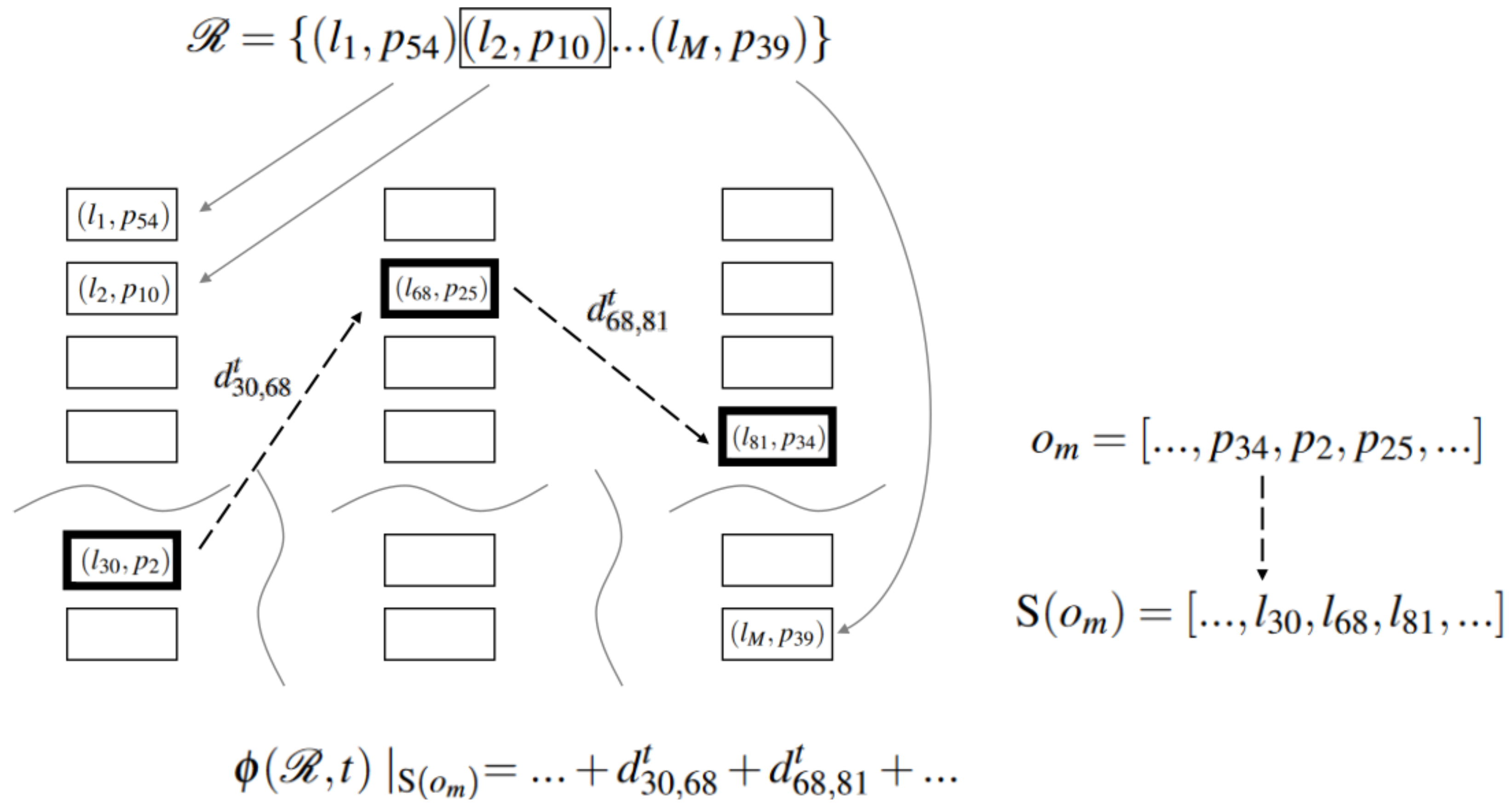
Figure 2 summarizes the formulation and exemplifies the binary relation location-product $\mathcal{R}$ as physical locations of the warehouse with its associated products. Each order, $o_m$, indicates the products to be collected, being the associated sequence $\mathrm{S}\left(o_m\right)$ required. This defines, for each product retrieval action, a stochastic operation cost $d_{lp}^t$ that contributes to the cost function $\varphi$. In the example illustrated in Figure 2, it is a simple linear relation. Finally, the total cost, aggregated for all orders, is the objective function to optimize, as described in Equation (2).

This generic formulation, in its present form, is not useful for directly constructing a linear or integer programming model, which is a common strategy for solving the SLAP problem using exact methods. Instead, it helps to develop the structure of an object-oriented programming code for studying the SLAP in a way that is compatible with a simulation model. There are some advantages to following this modeling approach that might gain traction in the future as increased computation power becomes even more accessible. The necessary mathematical rigor is present in the definition of the model in order to remove ambiguity and outline the hypothesis, but there is no need to overcomplicate the model numerically. The simplicity helps on at least two fronts: (i) the greater interpretability of the model, which is meant to aid managerial decision-making, and, therefore, can be better explained in a natural and transparent manner; and (ii) the greater flexibility when it comes to the practical implementation and adaptation of the model, specifically if it is intended to be connected to different dedicated commercial simulation tools available in the market, or employed in real use cases.

3.2. Additional Assumptions for the Considered SLAP Study

After formulating the generic static SLAP with orders, the purpose of this subsection is to provide greater detail about the specific problem under consideration and to make its assumptions explicit. In particular, this section discusses the type of warehouse, products, orders, and solutions to be considered.

3.2.1. Warehouse

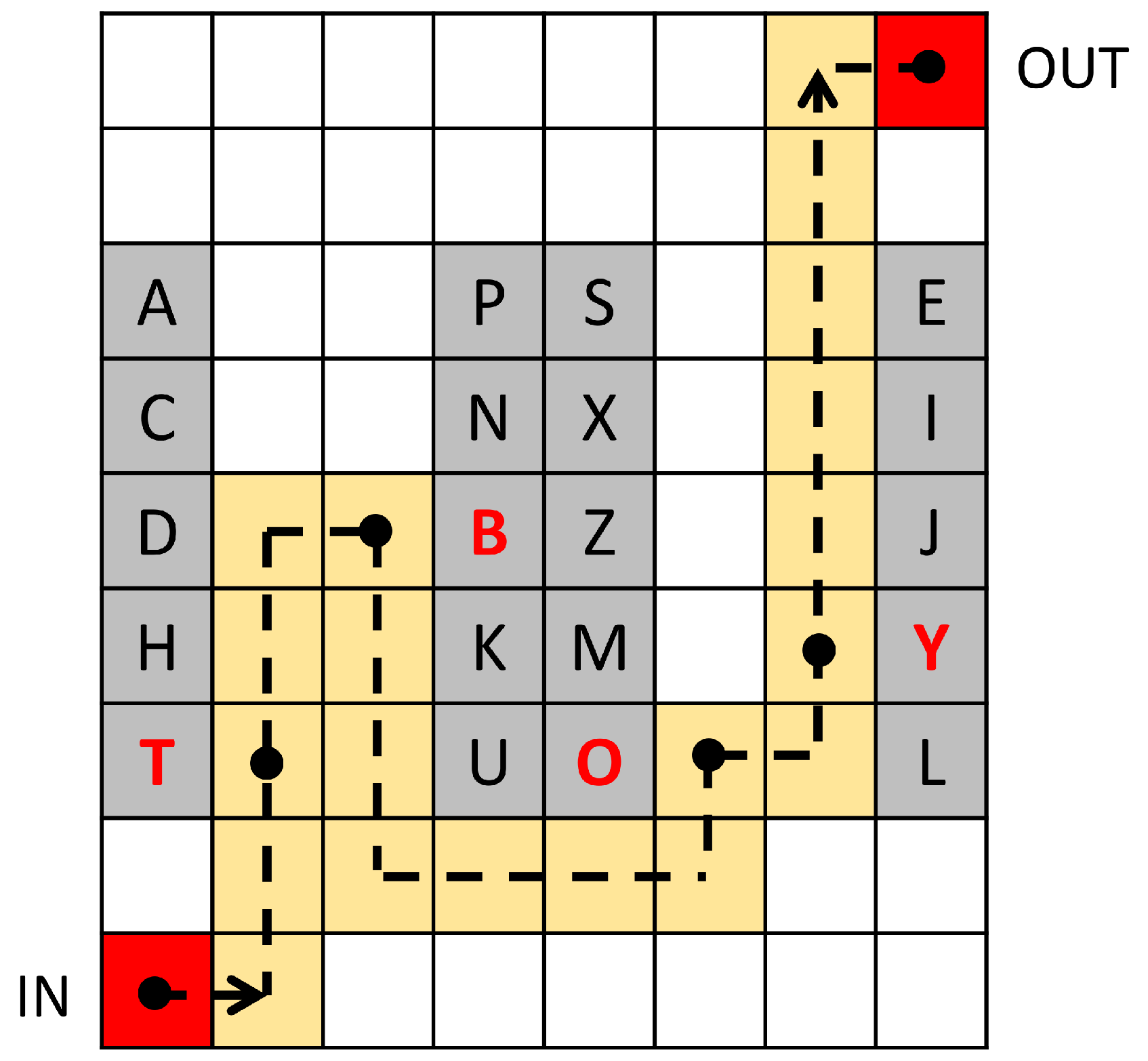
The SLAP in the present study is concerned with the placement of items in the so-called “picking slots”. Picking slots are designated areas for storing products in a unit or case format so that workers can retrieve (“pick”) the exact number of ordered units associated with each product. These picking slots are assumed to be either at the ground level or at the first level, with the rest of the rack height being dedicated to (non-picking) storage. This implies that the problem could be modeled in two dimensions (2D). Therefore, only the 2D characteristics of the warehouse were considered, i.e., the width and depth of corridors and distances in the horizontal plane. The warehouse modeled corresponds to a manual (i.e., non-automated) warehouse with a voice-assisted single-order picker-to-part system. This means that workers move through the warehouse with their actions guided by a warehouse management system (WMS), which tells them what products to collect next. Although more elaborated scenarios and picking strategies exist, the decision for this type of warehouse was based on the fact that this configuration is still very common in warehouses all around the world and that the simpler case (single-order picker-to-part) should be solved first before moving to more complex picking strategies. Figure 3 shows a very schematic representation of the warehouse abstraction that guided our warehouse modeling.

The inbound and outbound areas (where products are loaded and orders are dispatched, respectively) are assumed to be located at a certain fixed place in the warehouse and do not change within the studied planning horizon. Their position is, in that sense, a parametric decision that will affect the evaluation of the solution. Changing the input and output points generates a different solution space for the SLAP since changing where the completed orders need to be placed, or where workers start picking the next order, has an impact on the solution evaluation metrics (e.g., traveled distance). The effect of these inbound and outbound positions in the SLAP solution is usually neglected in most theoretical studies and is given as an unquestioned fixed input in the case studies in the literature. In the present study, however, we will consider the sensibility of the solution to the position of the input and output for the deterministic part of the simheuristic proposed.

3.2.2. Products

In this work, we assume that one type of product occupies exactly one storage location and that one storage location holds only one type of product. Further, the physical space of any storage location is sufficiently large for accommodating any quantity of items of the same type. Thus, the picking location replenishment activity could be ignored (i.e., there is always enough product available for picking). Additionally, it is assumed that there is enough capacity for the picker to retrieve all products from an order in a single route. Finally, all products have the same physical requirements for their storage (light, temperature, etc.), thus avoiding additional constraints that could be derived from this fact, such as dedicated zones for specific products.

3.2.3. Orders

In the scope of this investigation, the orders are defined as the ordered sequence of products to be retrieved from the warehouse in the form of lists. Each list contains a certain number of product requests that come from the same client (i.e., one order per client). The orders were assumed to follow the Pareto principle in the sense that roughly $80\%$ of the products that customers order correspond to just $20\%$ of warehouse references (unique products). Since the daily product demand from customers changes, the orders placed at the warehouse are considered a primary source of variability. No commercial agreements to serve fixed amounts of products according to a calendar were hypothesized.

3.2.4. Solution

In our study, the problem to be solved is a stochastic version of the static SLAP, which takes into account the uncertainty associated with the order placement from clients and the manual order-picking operation. The static SLAP considers that the proposed solution is to be kept throughout the entire planning horizon. In a dynamic version, instead of a fixed set of orders, these are received once they become available, and the system will need to respond and adapt dynamically to them. The metric to be optimized is the total distance covered by the warehouse workers in their picking routes. The potential sources of stochasticity in the problem will be indicated throughout the different paper sections, together with the parameters to be analyzed and tuned. For the Python model, the statistical variability will be limited to the orders, and for a selected set of orders, the behavior of the system will be fully deterministic. Within the FlexSim model, there will be multiple sources of stochasticity, reflecting a more realistic behavior of the system, such as the outbound point to place the finished orders or the interaction between workers.

4. Modeling Approach

This section presents the algorithmic implementation of the simheuristic framework and its different components, such as order generation,  warehouse navigation,  picking operation, and  solution evaluation. In the final subsections, the FlexSim implementation is briefly described, and the details of the solution method programmed are provided.

4.1. Simheuristic Framework

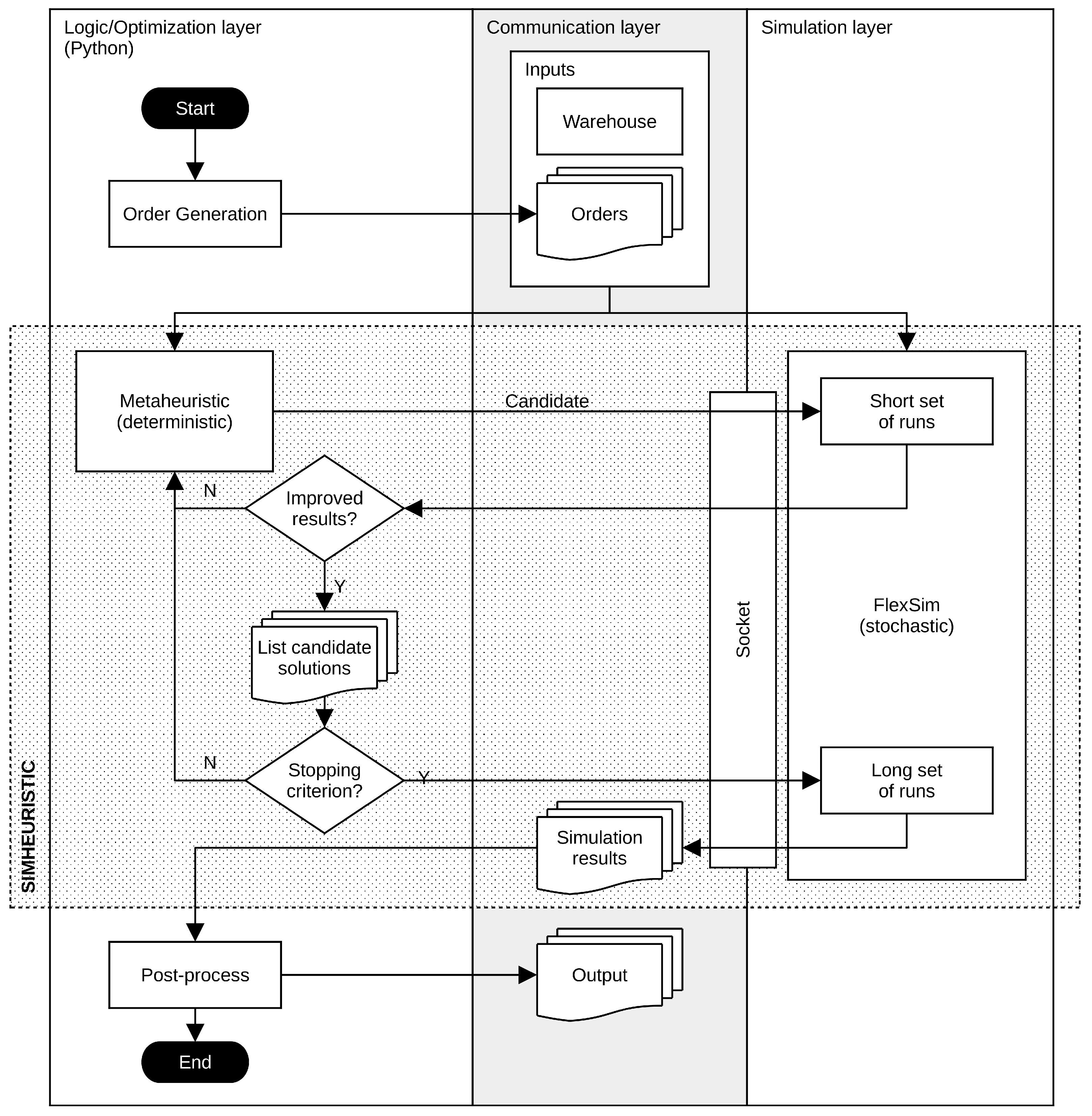
As outlined above, simheuristics belong to the family of simulation-optimization methods, and since they are applicable in many fields, they allow different levels of “intensity” in the interaction between the simulation and the optimization components. In the present study, the communication between both components was established using a well-established inter-process communication (IPC) protocol called “sockets”. This type of connection enables synchronous and flexible communication between two pieces of software, in this case, Python and FlexSim. All the details on how to establish this type of connection are presented in Leon et al. [32]. In that work, the researchers presented a very generic framework that allows information to be passed back and forth between a FlexSim simulation and a Python script. An asynchronous version of that same framework is to be used herein, where messages are passed at the beginning and the end of the FlexSim simulation. Figure 4 depicts the overall architecture of the work presented in the current study and the logic that its simheuristic part follows. In this case, we are calling simheuristic the part in charge of generating and evaluating solutions to the SLAP, excluding the data pre- and post-processing.

The simheuristic process begins by solving the deterministic version of the problem using a metaheuristic method programmed in Python (for more details, refer to Section 4.5). Given that the warehouse layout is known (as well as the assortment of products that it can hold), the other input required is the set of orders to be picked up. They can be real orders that are gathered and fed into the Python script, or they can be generated based, for instance, on a demand forecast for the period to be analyzed. The metaheuristic will produce candidate solutions that will be sent to FlexSim through the socket connection. The simulation model is configured exactly the same way as the deterministic model (same orders, warehouse layout, etc.), i.e., they share the same inputs. FlexSim then performs the simulation on each candidate storage location assignment and obtains a realistic evaluation of the objective function (total traveled distance). This process is repeated a certain number of times (a relatively small set of simulation runs or replications), producing different results due to its stochastic nature. These results are averaged and compared with one another in order to generate a list of candidate solutions, where the best-performing storage locations in both the deterministic and stochastic versions are kept. These elite candidate solutions are evaluated again in the stochastic FlexSim simulator using a larger number of replications. Finally, an analysis of the results is to be carried out. This final analysis, or post-processing, aims to assess the quality of each storage location assignment solution in terms of its performance and variability. It should be noted that the performance in the deterministic part is only assumed to be a proxy indication of the stochastic solution, and thus the performance of the solution in the stochastic simulator, after statistical treatment, is the true output of the simheuristic.

4.2. Order Generation

A Python module was created with the goal of simulating the orders that would be received at the warehouse. The orders are produced based on a pseudo-random number generator that takes into account various parameters as a generator seed: the date, the warehouse size, the number of products, and the number of orders (customers) to be served. This way of producing plausible orders allows them to be reproducible if the same parameters (same seed) are used. Creating exactly the same orders means that the instances can be potentially validated by other researchers. The order generator also takes into account the Pareto distribution associated with how frequently each product is requested from customers. If the information is available, these orders can be replaced with real orders from the warehouse under consideration. It is important to highlight the difference between the set of orders $\mathrm{O}$ (i.e., the lists containing the products to be retrieved for each customer) and the actual sequence of product retrieval $\mathrm{S}\left(o_m\right)$. The difference is that sequence $\mathrm{S}\left(o_m\right)$, as formulated in Section 3.1, contains more information than order $o_m$. Many equivalent orders can be generated by rearranging the products inside, but the optimized sequence is only one. The sequence is obtained from an order by applying a heuristic procedure at the same time that the solution is evaluated. This is explained in detail in Section 4.4.

4.3. Warehouse Navigation

The Python algorithm employed for evaluating the quality of different solutions (see Section 4.4) needs a deterministic way of calculating distances within the warehouse. These distances could be calculated using a simple metric—e.g., the Euclidian distance or the Manhattan distance. However, in order to make these distances realistic to some extent, the obstacles (mainly the racks) in the warehouse must be considered. It should be noted that the distances evaluated in the simulation component of the simheuristic (FlexSim) are considered real in the sense that they correspond to a unit of measure (e.g., meters) that has its own correspondence with the warehouse’s geometry. For the Python algorithm, only a realistic comparison between distances (or costs) is required. An option for the distance calculation that can consider obstacles could be the A-star ($A^{*}$) algorithm. This well-known path-finding algorithm has the advantage of being optimal, but it also has a major drawback, which is its exponential time and space complexity. Therefore, for large warehouse instances, the use of the $A^{*}$ algorithm could be impracticable. It is worthwhile to note that the term ‘path’ is used, in the context of this study, mainly to refer to the segments that connect two target points in the warehouse. The term ‘route’ is employed as the final path that joins the input and output points while collecting the products following the order sequence.

Given the scope of this study, a specific algorithm for navigating the warehouse has been proposed. The algorithm was dubbed W-star ($W^{*}$), where the W stands for warehouse and the ‘*’ symbol is a reminiscence of the $A^{*}$ navigating algorithm name. The main geometrical assumption made for the warehouse geometry was that the warehouse is “single-block”—i.e., made of same-length undivided racks. It was also assumed that there is a two square distance between both sides of the aisle in the discretization grid, that the start and end points are valid product positions, and that the racks are distributed along the vertical axis of the 2D warehouse. All this is shown in Figure 3. The pseudocode for the $W^{*}$ is shown in Algorithm 1. As opposed to $A^{*}$, the complexity of this algorithm is independent of the path length (since alternative paths do not need to be stored with every new node movement), allowing larger warehouse instances to be calculated within reasonable computing times.

Algorithm 1 W* algorithm.

Inputs: $warehouse$, $start$, $end$      Output: $path$ 1: for all direction: $<up>$, $<down>$ do 2:     while horizontal distance is not 0 do 3:         if moving horizontally towards end is allowed then 4:            move 1 step horizontally towards end 5:         else 6:            move 1 step vertically according to direction 7:     while vertical distance is not 0 do 8:         move vertically towards end 9: select shortest path: $<up>$ or $<down>$

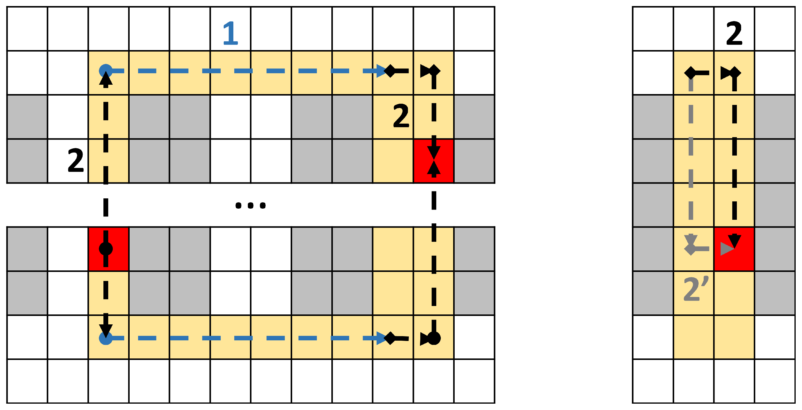
It can be proven that the proposed $W^{*}$ navigation algorithm provides high-quality solutions. The proof consists of dividing the path into two parts and showing that no better alternative is available for each part (see Figure 5). The first part is the movement around the racks. Since the racks cannot be traversed, this movement cannot be avoided, and it is performed in a straight horizontal line, which is the shortest path between the two points right above/below the racks. The second part is movement inside the corridors. This movement can be performed in multiple ways, but the traveled distance is minimal with the selected strategy (as with many others, but it cannot be smaller because diagonal movements are not allowed).

4.4. Picking Operation and Solution Evaluation

The picking or product retrieval operation constitutes the way in which the “goodness” of the storage location assignment performed can be evaluated, i.e., it is employed for the evaluation of the objective function (total traveled distance). In real life, the picking operation involves two elements: (i) the workers that perform the different tasks—their number, position, and characteristics, including speed, ability to turn around, etc.; and (ii) the strategy followed during the picking operation—the routing, the directions and areas allowed, and the sequence of actions. In the case studied in this paper, the picking operation was designed to be as similar as possible for both the optimization side of the algorithm programmed in Python and the simulation part modeled in FlexSim. As it can be expected, the picking operation on the simulation side would be much more detailed: the effects of congestion could be present, the movements required to face the racks and to remove items, although small, are taken into account, etc. In addition, on the optimization side, several simplifications had to be made.

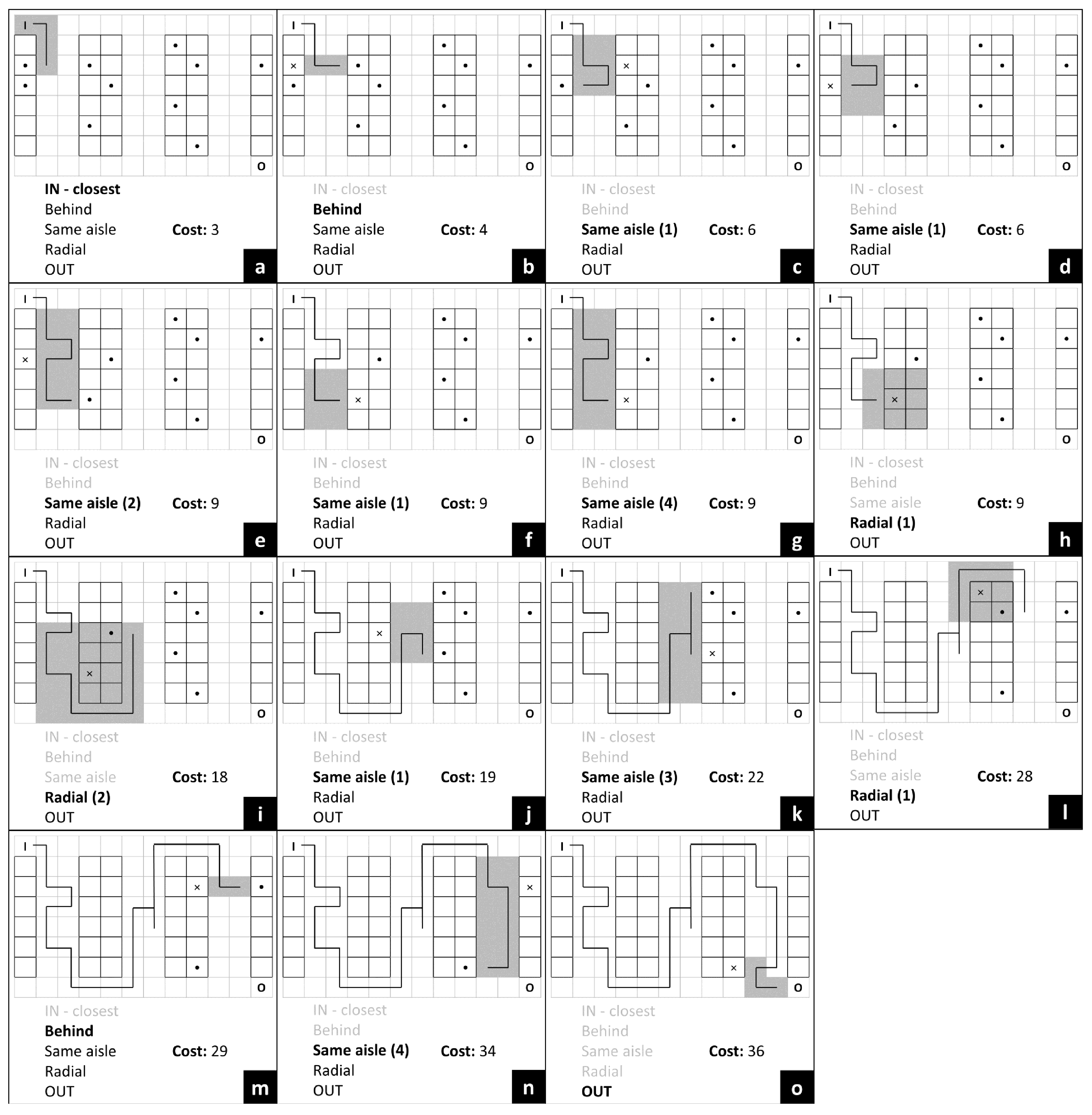
As for the picking strategy followed, the workers will always collect the items following the sequence of orders $\mathrm{S}\left(o_m\right)$. This means that the lists of orders must be rearranged in such a way that, when the picking operation is performed, a consistent and good strategy is followed. In reality, as long as the strategy is kept consistent, two solutions can be compared. In the literature, different picking or routing strategies have been proposed (S-shape, largest gap, return, etc.). These heuristics are widely used in practical applications (even more than optimal routing), and the strategy selection depends on the shape of the warehouse and the sparsity of the items [37]. In this particular work, no explicit order-picking routing was defined, but rather a simple set of rules from which the final strategy arises (Algorithm 2). The set of rules to construct the picking route start from the input point and find the closest location with a product using different strategies, always in the same order. If a product is found, then it is fixed in the retrieval sequence, and  the algorithm continues from that location. If no product is found, then the search resumes using the next rule. The search rules are (in order): (i) from the current location, look at the position right behind, in the same aisle; (ii) from the current location, look for the closest product within the same aisle; and (iii) from the current location, look for the closest product “radially”. Figure 6 shows a graphical description of this picking route construction strategy.

Algorithm 2 Evaluate Deterministic Solution.
Inputs: $SLA$, $orders$	▹ Storage Location Assignment
Outputs: $cost$, $sequence$	▹ Per order
1: $cost\leftarrow 0$ 2: for all $orders$ do 3:     $item\leftarrow$ empty 4:     while $order\ne$ empty do 5:         if $item$ = empty then
6:            $next\_item\leftarrow$ find_closest(IN)	▹ The route begins from the initial (“IN”) point
7:            $cost\leftarrow cost+$ distance(IN, $next\_item$) 8:         else 9:            $step\leftarrow$ 0 10:            while $next\_item=$ empty do
11:                $step\leftarrow step$ +1	▹ Every loop iteration the search step increases
12:                if behind($item$) ≠ empty then	▹ First: search behind
13:                    $next\_item\leftarrow$ behind($item$)
14:                else if length($item,step$) ≤ aisle_length then	▹ Second: search in the aisle
15:                    $next\_item\leftarrow$ search_in_aisle($step$) 16:                else
17:                    $next\_item\leftarrow$ search_round($step$)	▹ Third: search in a “round” fashion
18:            $cost\leftarrow cost+$ distance($item$, $next\_item$) 19:         remove $item$ from $order$ 20:         $sequence\leftarrow \mathrm{add}(item)$ 21:         $item\leftarrow next\_item$
22:     $cost\leftarrow cost+$ distance($item$, OUT)	▹ The route finishes at the final (“OUT”) point

It is important to notice that this strategy is a consistent (deterministic) and logical one that tends to minimize the total length of the route in most cases, but that does not guarantee its optimality. In fact, the process is a local greedy search process, and, in some storage location configurations, it will perform movements that a warehouse manager would deem inappropriate. Nonetheless, the advantage of following this approach is a drastic reduction in the computation complexity since calculations of distance matrices or performing various loops through the entire warehouse are avoided. The final shape of the route has a strong resemblance to the S-shape picking strategy (since it will try to complete an entire aisle before moving to the next), but depending on how scattered the orders are or the position of the input and output points, other behavior can develop. In fact, the algorithm allows for some tuning: in the phase where it searches for products within the same aisle, it could be forced to start the “radial” search earlier if the next product down the aisle is very far away. This is relevant for scattered storage locations in big warehouses and will produce something similar to a mid-point strategy. It is important to highlight that, apart from evaluating the cost of each SLAP solution in a deterministic way, Algorithm 2 also provides the sequence in which items have to be picked up for every order by the warehouse workers in the FlexSim simulation (and, potentially, in real life). The route-construction algorithm could be further improved. These improvements, which are outside the scope of this work, could include: (i) allowing the search pattern to look slightly ahead to avoid unnatural turns within the aisle (e.g., see movements i, j, and k in Figure 6, where items could have been picked up without turning inside the aisle), but avoiding looking too far ahead since this will significantly increase the computational time; and (ii) allowing an automatic adjustment of the search pattern shape instead of being purely linear/radial, so it can change and adapt to different warehouse and storage location assignment configurations.

4.5. A Simheuristic for Solving the Storage Location Assignment Problem

The core component for finding a satisfactory solution to the SLAP is the strategy employed to generate good-quality storage location assignments. The strategies followed for generating different SLAs are what allow the exploration of the solution space. In this study, both the random strategy and the picking frequency-based storage strategy (PFS) were adopted as the benchmark storage methods. In the former, items were assigned to a storage location randomly. In the latter, items with higher picking frequency were assigned to storage locations nearer to the input and output points. These two methods are some of the most typical strategies adopted by warehouse managers when facing the SLAP, and they represent two extremes of a spectrum—i.e., random assignment and dedicated assignment, with the so-called class-based assignment strategy lying in between. The picking frequency-based storage strategy represents a greedy (and deterministic) heuristic for assigning items to storage locations. It follows this simple sequence: (1) items are sorted in the provided set of orders by picking frequency; (2) locations are sorted by distance to the input and output points (the two distances are added); (3) items and locations are matched in strict order (i.e., the item with the higher picking frequency is assigned to the location closer to both the input and output points) until all of them have been placed. The simheuristic presented in this paper, which tries to improve the benchmark solutions, is based on a biased-randomized algorithm (BRA). The idea behind BRA is the incorporation of a certain degree of randomness into a greedy heuristic, thus only partially maintaining its original logic, in order to explore the vicinity of the greedy solution. In particular, whereas the greedy PFS algorithm builds solutions by sequentially selecting the items with the highest picking frequency, BRA applies a skewed probability distribution to the task of selecting the items. Specifically, the geometric probability distribution, with parameter $\beta \in (0,1)$, was employed to introduce the biased-randomized behavior into the greedy PFS. In practice, the ordered list of items by picking frequency is reconstructed assuming that the probability of an item remaining at position x is given by:

$$P(\mathrm{X}=x)={(1-\beta )}^x$$

(3)

After a fine-tuning process, the value for the parameter $\beta$ was selected randomly in a range between $0.5$ and $0.7$. These values tend to provide a good trade-off between uniformly randomizing the list ($\beta =1$) and not affecting the ordered list ($\beta =0$) in a wide range of optimization problems. The pseudocode in Algorithm 3 shows how biased randomization is applied to this particular storage location assignment problem. It follows the logic described above for the PFS algorithm but with a randomization stage. As a matter of fact, this randomization stage could also be used to generate a random storage location assignment (by using $\beta =1$) or to recover the strictly greedy PFS algorithm (by using $\beta =0$).

Algorithm 3 Biased Randomized Heuristic (BRA).
Inputs: $warehouse$, $orders$, $\beta$
Output: $SLA$	▹ Storage Location Assignment
1: $items\_list\leftarrow$order_items_by_freq(orders)	▹ Most frequent first
2: $locations\_list\leftarrow$order_locations_by_distance(warehouse)	▹ Closer to input and output first
3: while $items\_list$ ≠ empty do
4:     $items\_list\leftarrow \mathrm{randomize}(items\_list,\beta )$	▹ Biased randomization using geometric distribution with $\beta$
5:     $item\leftarrow \mathrm{first}(items\_list)$ 6:     $location\leftarrow \mathrm{first}(locations\_list)$ 7:     $sla\leftarrow \mathrm{add}(item,location)$ 8:     remove $item$ from $items\_list$ 9:     remove $location$ from $locations\_list$

The pseudocode shown in Algorithm 4 illustrates how the simheuristic works by utilizing the BRA and the FlexSim discrete-event simulation model. The overall scheme is also shown in Figure 4. The main idea behind the simheuristic is to generate a list of elite candidate solutions that will perform well both in the deterministic and stochastic versions of the problem. For that, after an initialization phase where the PFS greedy algorithm is used as a baseline, a number of improvement iterations are performed. In each iteration, the BRA procedure is called to generate a solution. The solution is first evaluated in terms of its deterministic performance, and only if the solution cost is reduced is the stochastic evaluation undertaken. This stochastic evaluation is performed by running a “short” simulation stage, where FlexSim is called a certain number of times, and the stochastic cost obtained for each call is averaged. Once the improvement iterations are finished, and the list of elite solutions is complete, an “intensive” evaluation stage takes place. The objective of this evaluation phase is to extract a curated estimation of the stochastic cost for each elite solution, so that the one with the smallest average cost can be selected as the output. Therefore, the required inputs for the simheuristic are: the number of iterations for computing BRA solutions, the $\beta$ parameter for randomizing the product lists, the warehouse instance with its layout, the orders to be processed, the number of replications for a fast simulation stage, and the number of replications for a more intensive simulation stage.

Algorithm 4 Simheuristic.
Inputs: $iterations$, $warehouse$, $orders$, $\beta$      Output: $best\_solution$
1: $initial\_SLA\leftarrow \mathrm{BRA}(warehouse,orders,\beta =0)$	▹$\beta$ = 0: greedy
2: $best\_solution.determ\_cost\leftarrow$ evaluate_determ_solution(initial_SLA, orders)	▹ see Algorithm 2
3: $best\_solution.stoch\_cost\leftarrow \mathrm{Simulation}(best\_solution,short)$	▹ fast simulation: $short$ number of replications
4: $best\_sol\_list\leftarrow \mathrm{add}\left(best\_solution\right)$	▹ list of elite solutions
5: for $iterations$ do 6:     $new\_SLA\leftarrow \mathrm{BRA}(warehouse,orders,\beta )$ 7:     $new\_solution.determ\_cost\leftarrow$ evaluate_determ_solution(new_SLA, orders) 8:     if $new\_solution.determ\_cost<best\_solution.determ\_cost$ then 9:         $new\_solution.stoch\_cost\leftarrow \mathrm{Simulation}(new\_solution,short)$ 10:         if $new\_solution.stoch\_cost<best\_solution.stoch\_cost$ then 11:            $best\_solution\leftarrow new\_solution$
12:            $best\_sol\_list\leftarrow \mathrm{update}\left(best\_solution\right)$	▹ update elite list to include new best solution
13: for all $solution$ in $best\_sol\_list$ do
14:     $solution.stoch\_cost\leftarrow \mathrm{Simulation}(solution,long)$	▹ intensive simulation: $long$ number of replications
15: $best\_solution\leftarrow \mathrm{best}\left(best\_sol\_list\right)$	▹ return solution with minimum stochastic cost

5. Computational Experiments

This section presents a number of computational experiments to evaluate the proposed method, i.e., the performance of the simheuristic is compared against three benchmark methods, namely the greedy PFS, the BRA, and the random strategies. The traveled distance covered to fulfill all order picking operations is used as the key performance indicator to compare the solutions. All implemented algorithms are coded in Python v3.8.10 and run on a Windows 10 operating system, with an i7-4500U CPU 2.40 GHz and 6 GB RAM. FlexSim version 22.1.2 was employed for the simulation model. Section 5.1 describes the instances and experiment settings. Section 5.3 provides the analysis of the computational results.

5.1. Experiment Setting

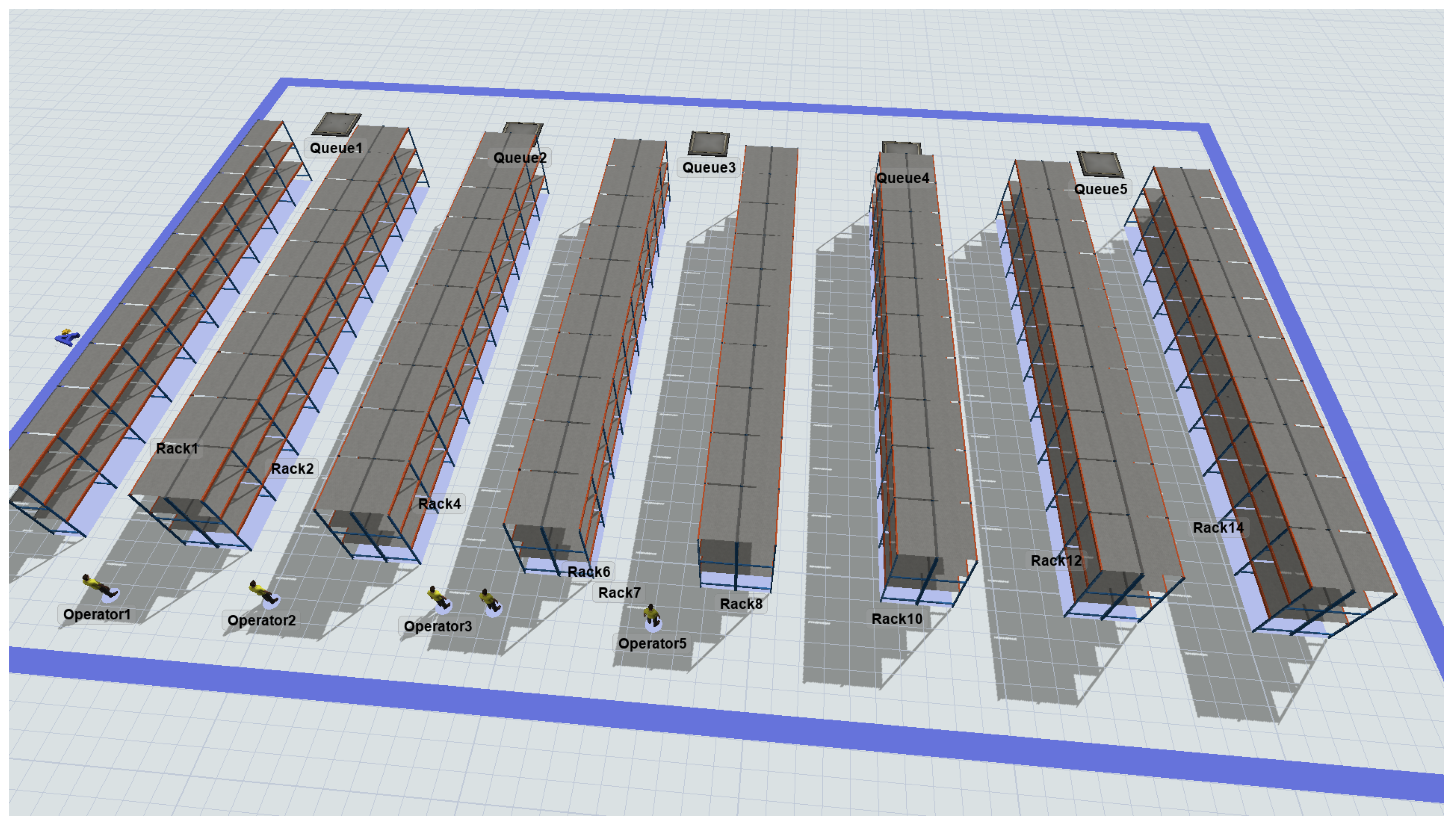
Two warehouse instances were tested for the numerical experiments. Instance A is composed of 15 racks with 10 slots each, capable of storing 150 unique products. Instance B is composed of 42 racks with 18 slots in each rack, capable of storing up to 756 unique products. The size of instance B is inspired by the one provided by Lee et al. [38]. The customer orders were generated using an independent Python script, which uses a fixed random seed for each calendar day to allow for reproducibility—i.e., on a given date and for a fixed set of parameters, the same set of orders can be produced by using the script. As described in Section 4.2, these orders follow the Pareto distribution, meaning that roughly $20\%$ of products will always be present in almost $80\%$ of the customer orders. In Figure 7, the implementation in FlexSim of instance A is shown. In terms of the number of runs, each solution obtained from the different methods studied is evaluated in the stochastic FlexSim environment using 10 replications, each of them employing a different random seed in order to obtain its associated stochastic cost. In order to make a fair comparison between the BRA method and the proposed simheuristic method, both were allowed to iterate 50 times in search of the best solution.

5.2. FlexSim Modeling

The functioning of the FlexSim stochastic model mirrors all the hypotheses made on the Python deterministic model, with some necessary differences. Those differences are, as a matter of fact, what makes the FlexSim simulation more realistic than the deterministic model. For instance, the navigation within the simulation model uses FlexSim’s own $A^{*}$ algorithm, which evaluates the minimum distances more truthfully since it can take into account all the obstacles present, specifically other workers. Another difference between both models is related to the start and end points of the picking routes. In the Python warehouse model, there is a single input point and a single output point, where pickers start collecting products and drop off collected products, respectively. In the FlexSim warehouse model, multiple output points are situated at one side of the warehouse, representing what in a real warehouse would be the dispatch area, being the starting point for picking up the next order is the last place where the worker left the previous finished order. This is indeed what happens in real life in most voice-assisted picking systems since there is no need for the worker to go to a specific place to receive the next order list. Lastly, depending on the instance used, the number of workers and output points varies. In a real-world application, the number of workers available for order picking can vary depending on the date (e.g., some workers might be on holiday or on sick leave), and, therefore, it could potentially be considered an additional stochastic input for the model. In the present case, the difference in the number of workers between instances and within the same instance was assumed to have a negligible effect. This is because most of the traveled distance is spent moving from item location to item location, and it would be only relevant if congestion within aisles became critical. Finally, the effect of the multiple output points in the simulation could be significant as the warehouse instances increase in size, thus amplifying the difference between the simulation and the deterministic model. This point will be discussed in Section 5.3.

5.3. Results and Discussion

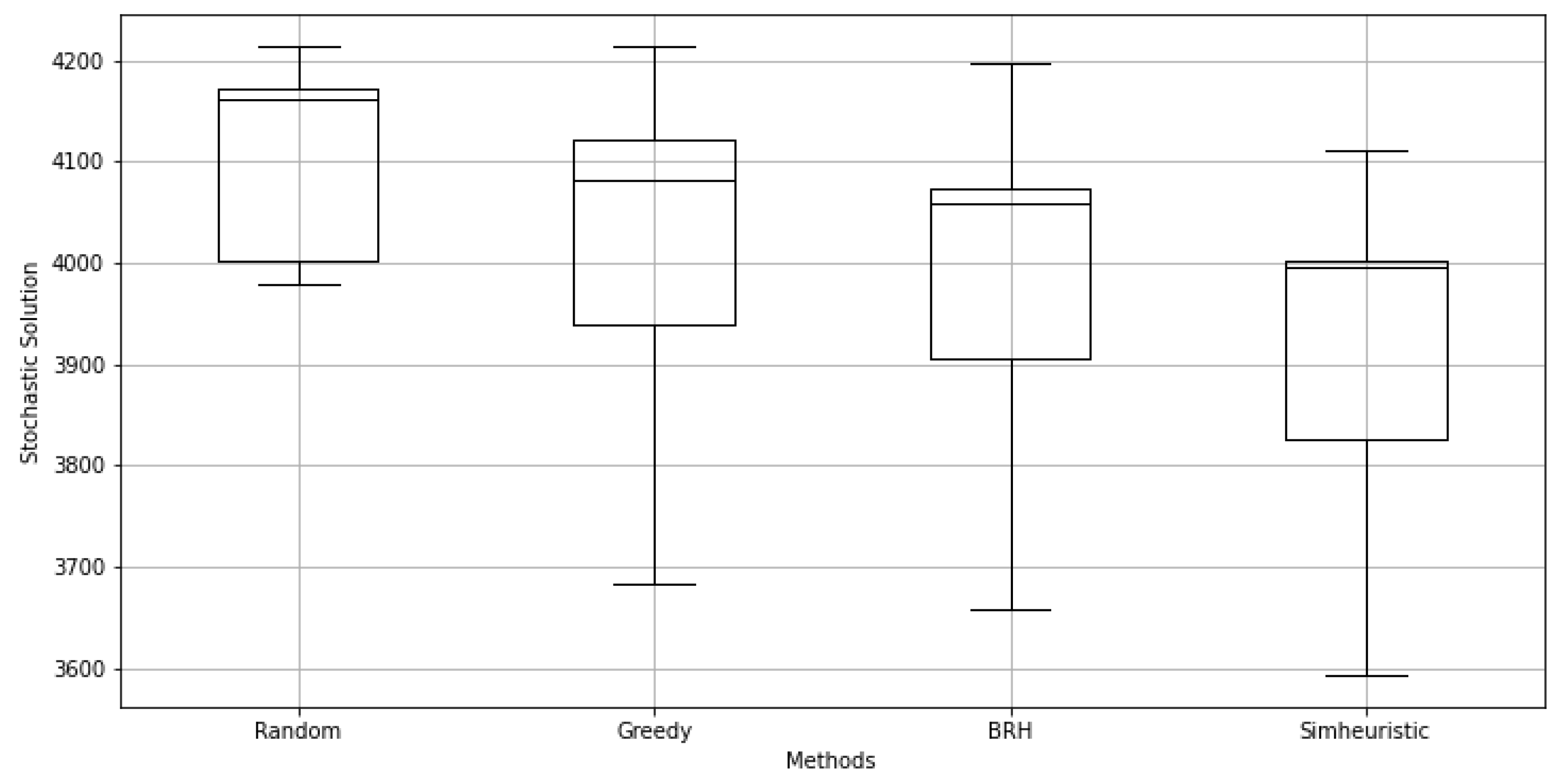
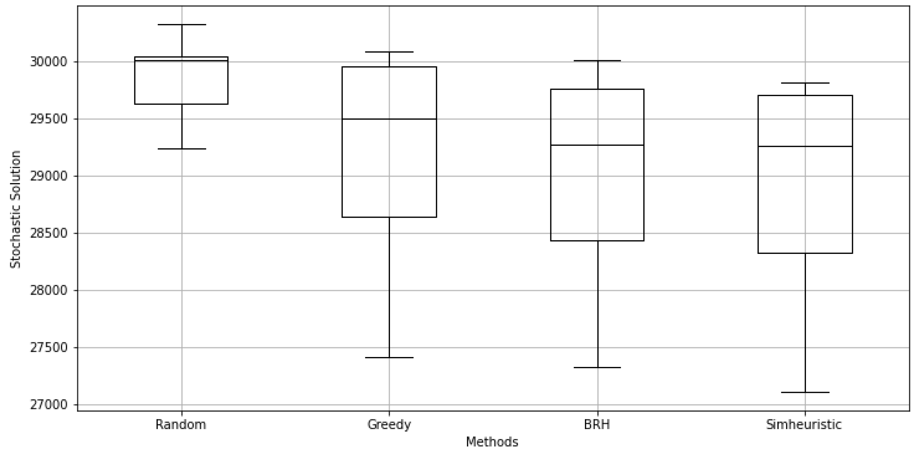
Due to the stochastic nature of the problem in real life, the results obtained were treated statistically by varying the set of orders. Warehouse instance A was tested using 10 different sets of orders, while instance B used only 3 different sets of orders because of its increased computational cost. This avoids improving the storage location assignment for a specific day or set of orders and increases confidence in the generated results. In order to further challenge the robustness of the simheuristic method, nine different combinations of input and output points were considered for the deterministic part of the simheuristic. In particular, all possible combinations between left (L), center (C), and right (R) positions for the input and output points were analyzed, as can be seen in

Table 1. Results comparison between different methods and gap to the simheuristic solution for instance A.

Warehouse Instance A
Input/Output	Random	Greedy	BRA	Simheuristic	Gap	Gap	Gap
	[1]	[2]	[3]	[4]	[1]–[4]	[2]–[4]	[3]–[4]
C / C	4163	4102	4058	3998	−4.0%	−2.5%	−1.5%
C / L	4171	3938	3905	3827	−8.2%	−2.8%	−2.0%
C / R	4128	4129	4074	3997	−3.2%	−3.2%	−1.9%
L / C	3985	3775	3710	3675	−7.8%	−2.6%	−0.9%
L / L	3978	3682	3658	3593	−9.7%	−2.4%	−1.8%
L / R	4003	3946	3936	3882	−3.0%	−1.6%	−1.4%
R / C	4167	4122	4076	4050	−2.8%	−1.7%	−0.6%
R / L	4191	4215	4197	4111	−1.9%	−2.5%	−2.0%
R / R	4214	4081	4059	4002	−5.0%	−1.9%	−1.4%
Average	4111	3999	3964	3904	−5.1%	−2.4%	−1.5%

and

Table 2. Results comparison between different methods and gap to the simheuristic solution for instance B.

Warehouse Instance B
Input/Output	Random	Greedy	BRA	Simheuristic	Gap	Gap	Gap
	[1]	[2]	[3]	[4]	[1]–[4]	[2]–[4]	[3]–[4]
C / C	30,013	29,497	29,272	29,317	−2.3%	−0.6%	0.2%
C / L	29,996	28,718	28,741	28,502	−5.0%	−0.8%	−0.8%
C / R	30,333	30,088	29,816	29,710	−2.1%	−1.3%	−0.4%
L / C	29,242	27,923	27,799	27,799	−4.9%	−0.4%	0.0%
L / L	29,320	27,414	27,322	27,106	−7.6%	−1.1%	−0.8%
L / R	29,629	28,647	28,434	28,330	−4.4%	−1.1%	−0.4%
R / C	30,049	29,964	29,768	29,814	−0.8%	−0.5%	0.2%
R / L	30,113	29,638	29,385	29,263	−2.8%	−1.3%	−0.4%
R / R	30,038	29,979	30,016	29,763	−0.9%	−0.7%	−0.8%
Average	29,859	29,096	28,950	28,845	−3.4%	−0.9%	−0.4%

. These tables show the traveled distance for each type of solution, for each combination of input and output points, averaged across the set of orders considered for each instance. The gap between the simheuristic solution and each of the benchmark solutions is computed as the percentage difference between them in order to evaluate their performance. Since the optimization goal is to minimize the traveled distances, a negative gap indicates that the simheuristic algorithm performed better in that case.

As can be seen in both tables, the simheuristic method consistently outperforms other methods, i.e., in the practical totality of cases, the traveled distance is less for the simheuristic method. However, in instance B, this difference in performance, even though it is present and globally in favor of the simheuristic, is much smaller. This can be seen graphically in both Figure 8 and Figure 9. The impact on the solutions of other parameters, such as the number of orders to be picked, was analyzed, but no significant effect was observed. The case where the number of products per order can be modified was also studied, but only the gap between the random method and the rest of the methods was affected. This means that, for shorter orders (fewer items to collect), the random policy could be a good option since it provides comparable results and its implementation is much simpler. On the other hand, with more items to collect per order, the greedy, BRA, and simheuristic methods showed a clear advantage. Nonetheless, the relative improvement between these three methods remained the same, with the simheuristic being the best among them.

It can be noticed that the random strategy results were less scattered when compared to the other methods. Moreover, the evaluation of the other methods had a similar level of variability. One reason for this is that the random solution will perform equally well (or poorly) with the independence of the stochastic variability present in the FlexSim simulator and hence be less sensitive. On the other hand, solutions that are more optimal in the deterministic version of the problem could suffer from higher variability in the results when evaluated in a stochastic environment. For instance, the deterministic solution could rely on workers always starting their picking route close to one side of the warehouse, but in the stochastic model, products might be required to be sometimes dropped at the other end of the warehouse, destroying the advantage of the deterministic solution. Although the simheuristic has a similar level of variability, it tends to be biased towards minimizing the traveled distance.

The results also show that the capacity of the simheuristic to improve the BRA results in warehouse instance B (the larger one) is reduced when compared to warehouse A. The main reason for this could be the presence of additional input and output points in the FlexSim model compared to the three points in the deterministic model (left, center, right). Nonetheless, this is a direct consequence of the size of the warehouse, i.e., in most real situations, the bigger the warehouse, the larger the outbound area. It is very unlikely to find studies in the literature that do consider this fact: in a real warehouse, the outbound area looks more like a continuous section of the warehouse rather than a single point. This study considers that the FlexSim stochastic environment represents a closer-to-reality picture of the warehouse, and the deterministic model is the tool that allows the efficient exploration of the optimization space. It is clear that, as the deterministic and stochastic models become more dissimilar, the correlation between them will diminish, as will the effectiveness of the method.

Lastly, the fact that the optimization results will depend on the set of orders analyzed has very interesting consequences. On the one hand, if this fact were assumed rigidly, it would not be practical since it would mean changing the warehouse configuration with every set of orders received. On the other hand, a more flexible interpretation of this fact could result in a very useful managerial tool. For instance, the set of orders to be analyzed could be prepared beforehand to represent the historical demand in the warehouse or could be used to analyze “what-if” scenarios. In those cases, the methodology used in this study provides a robust storage location assignment that tends to minimize warehouse traveled distance for that given set of orders. As a result, decision-makers could compare the warehouse’s current configuration to the results proposed by the simheuristic and take appropriate action. In other words, it allows the investigation of stochastically robust solutions for a profile of orders of interest.

6. Conclusions and Future Work

This paper provides a simheuristic algorithm based on a static and deterministic formulation of the storage location assignment problem (i.e., orders are processed for a fixed time horizon, as opposed to orders received dynamically), which considers the picking frequency of products in the orders as the main optimization driver. Multiple deterministic solutions are generated using a biased randomization procedure and evaluated in a FlexSim simulator in order to extract a number of candidate solutions that minimize the stochastic traveled distance. These elite solutions are thoroughly tested in the same commercial simulator in order to find the best configuration. This method represents a simple and natural way to improve the deterministic solution by ensuring that it will also perform well under realistic conditions. The capacity of our simheuristic approach to finding high-quality solutions depends crucially on the similarity between the deterministic model and the stochastic model. Trying to achieve greater similarity between both could mean that the deterministic model needs to be more complex (and hence more difficult to optimize) or that the stochastic model needs to be simplified (and hence less realistic). Finding a sweet spot between both is difficult. In this study, a relatively complex deterministic model was developed in order to keep a stochastic model as realistic as possible (e.g., multiple input and output points, large-size instances, etc.). The positive results found have been verified under different input conditions and warehouse instances, with the simheuristic outperforming the benchmark methods considered in the practical totality of them.

In practical terms, the simheuristic algorithm allows managers to obtain a robust solution to the configuration of locations and products in a warehouse while also considering the uncertainty associated with the stochastic processes involved. This means that a decision-maker could obtain, for the evaluated time horizon, an improved warehouse configuration with the goal of minimizing total worker travel distance. Based on this proposed configuration and the current state of the warehouse and its associated business metrics (e.g., the cost of changing a product’s location, the risk of a supply shortage, relationships with clients, etc.), the decision-maker could then choose the best course of action. The implementation of the proposed solution as part of a warehouse management system (WMS) could be considered a very interesting practical application of the research presented here.

From the presented results and conclusions, a number of future lines of work can be highlighted. These lines of work could be separated into three areas: (i) improving the deterministic model; (ii) improving the simheuristic algorithm; and (iii) improving the applicability of the method. Regarding improvements in the deterministic model, the SLAP formulation could be extended in multiple ways, with the aim of achieving a higher level of realism. In this paper, a basic version of a voice-assisted single-order picker-to-part square warehouse was modeled, which is a common configuration, but it is recognized that in practical use cases, more complicated warehouse configurations can be found. For instance, the model could include more complex picking strategies, such as multi-order (batch) picking, or include additional restrictions, such as considering different degrees of compatibility between products and locations. In relation to the simheuristic framework, it could be improved by exploiting the data available in the simulation more effectively, with the objective of guiding the metaheuristic procedure better. In the present work, the traveled distance was used, but there is a good deal of unexplored information available in the simulation (e.g., resource utilization, average speed, etc.) that could be potentially employed. This is indeed a very promising research line, but one that requires careful design and implementation, specifically the communication between the two pieces of software and the simulation-optimization framework selected. An example of this line of research could be developing a metaheuristic procedure that invokes the simulation environment at specific points of the solution search in order to evaluate the current solution, extract some metrics from the simulation model, and decide, in consequence, the next area to explore in the solution space. With regard to the integration and application of this work, it could be extended by defining a complete data workflow, from inputs to final output formats, which could be most useful for managers to make decisions or for allowing the integration of the simheuristic into a warehouse management system, as pointed out previously. Finally, as highlighted in Silva et al. [13], the lack of benchmark instances for comparing different methods could be addressed by further developing the idea hinted at in this study of generating a reproducible set of orders. These sets of orders, which are generated based on certain inputs (simple ones, such as the calendar day and the dimensions of the warehouse), could allow different researchers to share the same problem definition and be able to compare solutions.

References

1. Zhang, R.Q.; Wang, M.; Pan, X. New model of the storage location assignment problem considering demand correlation pattern. Comput. Ind. Eng. 2019, 129, 210–219. [Google Scholar] [CrossRef]
2. Reyes, J.; Solano-Charris, E.; Montoya-Torres, J. The storage location assignment problem: A literature review. Int. J. Ind. Eng. Comput. 2019, 10, 199–224. [Google Scholar] [CrossRef]
3. Chica, M.; Juan, A.A.; Bayliss, C.; Cordón, O.; Kelton, W.D. Why simheuristics? Benefits, limitations, and best practices when combining metaheuristics with simulation. SORT Stat. Oper. Res. Trans. 2020, 44, 311–334. [Google Scholar] [CrossRef] [Green Version]
4. van Rossum, G.; Drake, F.L. Python 3 Reference Manual; CreateSpace: Scotts Valley, CA, USA, 2009. [Google Scholar]
5. Nordgren, W.B. FlexSim Simulation Environment. In Proceedings of the 2002 Winter Simulation Conference, San Diego, CA, USA, 8–11 December 2002; pp. 250–252. [Google Scholar] [CrossRef]
6. Tendeloo, Y.V.; Vangheluwe, H. Discrete event system specification modeling and simulation. In Proceedings of the 2018 Winter Simulation Conference, Gothenburg, Sweden, 9–12 December 2018; pp. 162–176. [Google Scholar] [CrossRef]
7. Amorim-Lopes, M.; Guimarães, L.; Alves, J.; Almada-Lobo, B. Improving picking performance at a large retailer warehouse by combining probabilistic simulation, optimization, and discrete-event simulation. Int. Trans. Oper. Res. 2021, 28, 687–715. [Google Scholar] [CrossRef]
8. Kofler, M. Optimising the Storage Location Assignment Problem under Dynamic Conditions. Ph.D. Thesis, JKU—Johannes Kepler Universität Linz, Linz, Austria, 2015. [Google Scholar]
9. Fumi, A.; Scarabotti, L.; Schiraldi, M.M. Minimizing Warehouse Space with a Dedicated Storage Policy. Int. J. Eng. Bus. Manag. 2013, 5, 21. [Google Scholar] [CrossRef] [Green Version]
10. Xie, J.; Mei, Y.; Ernst, A.T.; Li, X.; Song, A. A genetic programming-based hyper-heuristic approach for storage location assignment problem. In Proceedings of the 2014 Congress on Evolutionary Computation (CEC), Beijing, China, 6–11 July 2014; pp. 3000–3007. [Google Scholar] [CrossRef]
11. Chen, L.; Langevin, A.; Riopel, D. A Tabu search algorithm for the relocation problem in a warehousing system. Int. J. Prod. Econ. 2011, 129, 147–156. [Google Scholar] [CrossRef]
12. Boysen, N.; de Koster, R.; Weidinger, F. Warehousing in the e-commerce era: A survey. Eur. J. Oper. Res. 2019, 277, 396–411. [Google Scholar] [CrossRef]
13. Silva, A.; Coelho, L.C.; Darvish, M.; Renaud, J. Integrating storage location and order picking problems in warehouse planning. Transp. Res. Part E Logist. Transp. Rev. 2020, 140, 102003. [Google Scholar] [CrossRef]
14. Mantel, R.J.; Schuur, P.C.; Heragu, S.S. Order oriented slotting: A new assignment strategy for warehouses. Eur. J. Ind. Eng. 2007, 1, 301–316. [Google Scholar] [CrossRef]
15. Keung, K.L.; Lee, C.K.M.; Ji, P. Data-driven order correlation pattern and storage location assignment in robotic mobile fulfillment and process automation system. Adv. Eng. Inform. 2021, 50, 101369. [Google Scholar] [CrossRef]
16. Keung, K.L.; Lee, C.K.M.; Ji, P. Industrial internet of things-driven storage location assignment and order picking in a resource synchronization and sharing-based robotic mobile fulfillment system. Adv. Eng. Inform. 2022, 52, 101540. [Google Scholar] [CrossRef]
17. Zhang, G.; Shang, X.; Alawneh, F.; Yang, Y.; Nishi, T. Integrated production planning and warehouse storage assignment problem: An IoT assisted case. Int. J. Prod. Econ. 2021, 234, 108058. [Google Scholar] [CrossRef]
18. Lanza, G.; Passacantando, M.; Scutellà, M.G. Assigning and sequencing storage locations under a two level storage policy: Optimization model and matheuristic approaches. Omega 2022, 108, 102565. [Google Scholar] [CrossRef]
19. Xu, X.; Ren, C. A novel storage location assignment in multi-pickers picker-to-parts systems integrating scattered storage, demand correlation, and routing adjustment. Comput. Ind. Eng. 2022, 172, 108618. [Google Scholar] [CrossRef]
20. Guo, X.; Chen, R.; Du, S.; Yu, Y. Storage assignment for newly arrived items in forward picking areas with limited open locations. Transp. Res. Part E Logist. Transp. Rev. 2021, 151, 102359. [Google Scholar] [CrossRef]
21. Montanari, R.; Micale, R.; Bottani, E.; Volpi, A.; La Scalia, G. Evaluation of routing policies using an interval-valued TOPSIS approach for the allocation rules. Comput. Ind. Eng. 2021, 156, 107256. [Google Scholar] [CrossRef]
22. Juan, A.A.; Keenan, P.; Martí, R.; McGarraghy, S.; Panadero, J.; Carroll, P.; Oliva, D. A review of the role of heuristics in stochastic optimisation: From metaheuristics to learnheuristics. Ann. Oper. Res. 2021, 320, 831–861. [Google Scholar] [CrossRef]
23. Bianchi, L.; Dorigo, M.; Gambardella, L.M.; Gutjahr, W.J. A survey on metaheuristics for stochastic combinatorial optimization. Nat. Comput. 2009, 8, 239–287. [Google Scholar] [CrossRef] [Green Version]
24. Rabe, M.; Deininger, M.; Juan, A.A. Speeding up computational times in simheuristics combining genetic algorithms with discrete-event simulation. Simul. Model. Pract. Theory 2020, 103, 102089. [Google Scholar] [CrossRef]
25. Figueira, G.; Almada-Lobo, B. Hybrid simulation–optimization methods: A taxonomy and discussion. Simul. Model. Pract. Theory 2014, 46, 118–134. [Google Scholar] [CrossRef] [Green Version]
26. Castaneda, J.; Martin, X.A.; Ammouriova, M.; Panadero, J.; Juan, A.A. A Fuzzy Simheuristic for the Permutation Flow Shop Problem under Stochastic and Fuzzy Uncertainty. Mathematics 2022, 10, 1760. [Google Scholar] [CrossRef]
27. Antoniadis, N.; Cordy, M.; Sifaleras, A.; Le Traon, Y. A variable neighborhood search simheuristic algorithm for reliability optimization of smart grids under uncertainty. Int. Trans. Oper. Res. 2022, 29, 2172–2200. [Google Scholar] [CrossRef]
28. Hatami, S.; Calvet, L.; Fernandez-Viagas, V.; Framinan, J.M.; Juan, A.A. A simheuristic algorithm to set up starting times in the stochastic parallel flowshop problem. Simul. Model. Pract. Theory 2018, 86, 55–71. [Google Scholar] [CrossRef]
29. Ferone, D.; Hatami, S.; González-Neira, E.M.; Juan, A.A.; Festa, P. A biased-randomized iterated local search for the distributed assembly permutation flow-shop problem. Int. Trans. Oper. Res. 2020, 27, 1368–1391. [Google Scholar] [CrossRef]
30. Bayliss, C.; Guidotti, R.; Estrada-Moreno, A.; Franco, G.; Juan, A.A. A biased-randomized algorithm for optimizing efficiency in parametric earthquake (re) insurance solutions. Comput. Oper. Res. 2020, 123, 105033. [Google Scholar] [CrossRef]
31. Nordgren, W.B. FlexSim simulation environment. In Proceedings of the 2003 Winter Simulation Conference, New Orleans, LA, USA, 7–10 December 2003; Volume 1, pp. 197–200. [Google Scholar] [CrossRef]
32. Leon, J.F.; Peyman, M.; Li, Y.; Dehghanimohammadabadi, M.; Calvet, L.; Marone, P.; Juan, A.A. A Tutorial On Combining FlexSim With Python For Developing Discrete-Event Simheuristics. In Proceedings of the 2022 Winter Simulation Conference, Singapore, 11–14 December 2022. [Google Scholar]
33. Zhu, X.; Zhang, R.; Chu, F.; He, Z.; Li, J. A Flexsim-based Optimization for the Operation Process of Cold-Chain Logistics Distribution Centre. J. Appl. Res. Technol. 2014, 12, 270–278. [Google Scholar] [CrossRef] [Green Version]
34. Wu, G.; Yao, L.; Yu, S. Simulation and optimization of production line based on FlexSim. In Proceedings of the 2018 Chinese Control and Decision Conference (CCDC), Shenyang, China, 9–11 June 2018; pp. 3358–3363. [Google Scholar] [CrossRef]
35. Pan, J.C.H.; Shih, P.H.; Wu, M.H.; Lin, J.H. A storage assignment heuristic method based on genetic algorithm for a pick-and-pass warehousing system. Comput. Ind. Eng. 2015, 81, 1–13. [Google Scholar] [CrossRef]
36. Jiao, Y.L.; Xing, X.C.; Zhang, P.; Xu, L.C.; Liu, X.R. Multi-objective storage location allocation optimization and simulation analysis of automated warehouse based on multi-population genetic algorithm. Concurr. Eng. 2018, 26, 367–377. [Google Scholar] [CrossRef]
37. Koster, R.D.; Poort, E.V.D. Routing orderpickers in a warehouse: A comparison between optimal and heuristic solutions. IIE Trans. 1998, 30, 469–480. [Google Scholar] [CrossRef] [Green Version]
38. Lee, I.G.; Chung, S.H.; Yoon, S.W. Two-stage storage assignment to minimize travel time and congestion for warehouse order picking operations. Comput. Ind. Eng. 2020, 139, 106129. [Google Scholar] [CrossRef]
Figure 1. Different SLAP policies: (a) random—products are assigned to storage locations randomly; (b) class-based—the warehouse is divided into product class zones, and each product is placed randomly within its class zone; (c) dedicated—products are assigned strictly based on certain characteristics, such as volume, turnover, or (as in this study) picking frequency.
Mathematics 11 01577 g001
Figure 2. The different components of the SLAP studied, showing an instance as an illustrative example.
Mathematics 11 01577 g002
Figure 3. Schematic 2D representation of the SLAP main ingredients: a space discretization, an initial (IN) and final (OUT) point, a storage location assignment of product to slots, a number of products to be retrieved (order products—letters in red color), and the corresponding picking route (IN, T, B, O, Y, OUT).
Mathematics 11 01577 g003
Figure 4. Description of the simheuristic framework logic.
Mathematics 11 01577 g004
Figure 5. The movement around the racks (1) is the shortest, trivially. The movement within the aisle (2) is also minimal. Other paths within the aisle can be found (2’) but the length would be the same or larger.
Mathematics 11 01577 g005
Figure 6. Graphic description of the sequence followed to construct the picking route. From the start point (step a) to the end point (step o), different search rules are applied, as explained in Algorithm 2: search behind (steps b and m), search within the aisle (steps c, d, e, f, g, j, k and n) and search radially (steps h, i and l).
Mathematics 11 01577 g006
Figure 7. FlexSim screenshot of instance A ( 15 × 10 ).
Mathematics 11 01577 g007
Figure 8. The average distance of stochastic versions of various methods for instance A.
Mathematics 11 01577 g008
Figure 9. The average distance of stochastic versions of various methods for instance B.
Mathematics 11 01577 g009