Reducing the Dimensionality of SPD Matrices with Neural Networks in BCI

Abstract

In brain–computer interface (BCI)-based motor imagery, the symmetric positive definite (SPD) covariance matrices of electroencephalogram (EEG) signals with discriminative information features lie on a Riemannian manifold, which is currently attracting increasing attention. Under a Riemannian manifold perspective, we propose a non-linear dimensionality reduction algorithm based on neural networks to construct a more discriminative low-dimensional SPD manifold. To this end, we design a novel non-linear shrinkage layer to modify the extreme eigenvalues of the SPD matrix properly, then combine the traditional bilinear mapping to non-linearly reduce the dimensionality of SPD matrices from manifold to manifold. Further, we build the SPD manifold network on a Siamese architecture which can learn the similarity metric from the data. Subsequently, the effective signal classification method named minimum distance to Riemannian mean (MDRM) can be implemented directly on the low-dimensional manifold. Finally, a regularization layer is proposed to perform subject-to-subject transfer by exploiting the geometric relationships of multi-subject. Numerical experiments for synthetic data and EEG signal datasets indicate the effectiveness of the proposed manifold network.

1. Introduction

As a system for connecting human brains and external devices, the brain–computer interface (BCI)-based motor imagery aims at converting the electroencephalogram (EEG) signals used to measure brain activity to computer commands [1]. Most BCIs rely on classification algorithms that can automatically extract features of EEG signals to achieve signal recognition, such as the famous common spatial pattern (CSP) [2]. However, some properties of EEG signals make it difficult [3], for instance, noise, outliers, high dimensionality, non-stationary, and small sample sets. It is well known that the space of symmetric positive definite (SPD) covariance matrices is a Riemannian manifold endowed with a Riemannian metric, which is a perspective to deal with the difficulties mentioned above. Recently, classification algorithms based on Riemannian geometry have demonstrated superior performance [4]. One of the major challenges of using those Riemannian approaches is the high dimensionality of EEG.

Some potential errors, such as swelling and non-complete space, may exist in Euclidean geometry. In contrast, the Riemannian manifold provides a comprehensive mathematical framework and copes with the limitations of Euclidean geometry. Consequently, exploring Riemannian geometry to describe EEG signals has attracted increasing interest. Compared with traditional signal classification methods such as estimating spatial filters and selecting features, the core idea of a Riemannian geometry classifier [5,6] is to utilize remarkable geometric properties to directly manipulate the SPD covariance matrices on the original manifold and perform classification based on their inherent geometric information. For example, Riemannian distance and Riemannian mean are robust to noise and outliers, which naturally lead minimum distance to the Riemannian mean (MDRM) classifier. In addition, tangent space at the geometric mean is the best hyperplane for classification [7], as a consequence of which projecting the data points to a tangent space [8,9,10] is another class of effective Riemannian approaches to extract features.

However, covariance matrices usually lie on a manifold with a smaller intrinsic dimensionality. The actual dimension of covariance matrices grows quadratically with the number of sampled signal channels. On the one hand, a systematic error [11] in estimating covariance matrices and heavy computation is inevitable on high-dimensional SPD manifolds, which limits the ability of BCI. On the other hand, classification in high-dimensional situations suffers from problems such as over-fitting and the curse of dimensionality. A practical approach to overcome the problems above is to reduce dimension, i.e., find a more compact low-dimensional representation from high-dimensional space.

Manifold learning is a class of non-linear dimensionality reduction methods based on the concept of the topological manifold. Canonical manifold learning approaches such as isometric mapping [12] and locally linear embedding [13] can not obtain an explicit mapping from the original space to the embedding that can be applied to new samples with an unknown relationship to training samples. Moreover, these manifold learning approaches based on vector form have to transform matrices into vectors, which leads to breaking the inherent spatial structure of the original matrix space. Fortunately, explicit bilinear mapping [14] for SPD matrix not only keeps the symmetric positive definiteness of the mapped matrix but also preserves the structure of a differentiable Riemannian manifold. More recently, linearization of traditional manifold learning methods [15,16] has been applied to reduce the dimensionality of the covariance SPD matrix. According to the purpose of preserving the intrinsic geometric structure, the classification performances after the above manifold learning methods based on bilinear mapping mainly depend on whether the original data is separable.

In contrast to preserving the geometric structure, by learning a suitable distance or similarity metric from data, metric learning methods finally find a more appropriate low-dimensional space than the original space, which is beneficial for various subsequent tasks. Riemannian metric learning on space of SPD matrices is a promising approach to make covariance matrices with manifold structure more interpretable [4]. The metric learning approaches [17,18,19,20,21] based on Riemannian geometry also use bilinear mapping, which can be considered as shallow learning. So, it is natural to consider if a bilinear mapping can also be extended to non-linear mapping.

In BCI, deep learning has not yet demonstrated its strong ability for EEG signal classification due to limited training data [5]. However, extensive research has been devoted to dimensionality reduction based on neural networks in the sense of similarity metric. To overcome the shortcomings of non-linear dimensionality reduction techniques, LeCun et al. [22,23] used the Siamese architecture to learn a similarity metric through a globally coherent non-linear function from the original data to low-dimensional vector manifolds. As an extension of the Siamese network, the Triplet network exhibits better performance under the same conditions [24], and FaceNet [25] is one of the typical examples of the Triplet network. More importantly, convolutional neural networks can effectively extract image features, drastically decreasing the difficulty of learning similarity measures. In non-linear dimensionality reduction for covariance matrices, the vectorization of the SPD matrices usually destroys the geometry structure of manifolds. It arouses a sequence of papers concerning manifold-to-manifold networks tailored for SPD matrices that use the paradigms of traditional neural networks. Huang et al. proposed the pioneering manifold network structures SPD-Net [26], which introduced some suitable non-linear layers to increase the complexity of learning as well as learn the potential geometric information at a deeper level. Subsequently, Zhang et al. [27] designed several layers without high-computational SVD operations and proposed a deep manifold-to-manifold transforming the network. Similarly, Dong et al. [28] constructed a deep neural network consisting of a 2D fully connected layer and a symmetrically clean layer to achieve non-linear dimensionality reduction. In general, the intersection of Riemannian geometry and neural networks opens up a new direction of non-linear learning in the deep manifold network.

In this paper, we design a novel non-linear mapping layer to shrink the extreme eigenvalues of the SPD covariance matrix, which can counteract the systematic bias. We then combine the non-linear shrinkage layer and traditional bilinear mapping layer to achieve non-linear dimensionality reduction in the SPD manifolds. Inspired by the successful paradigm of Siamese networks for vector-form metric learning, we learn the similarity metric by the contrast loss function, which aims to minimize Riemannian distances between similar signal covariance matrices while maximizing the distances between the dissimilar ones on the target manifold.

The main contribution of this paper is exploring the Siamese architecture to implement metric learning on Riemannian manifolds. In addition, a non-linear shrinkage layer for compensating the systematic bias is introduced to the manifold network for the first time. It is worthwhile to note that the output matrices of each layer in our network still flow on Riemannian manifolds so that we can use an efficient MDRM algorithm directly on the low-dimensional manifold rather than an end-to-end way. Furthermore, we reuse the geometric similarity metric of the covariance matrix in multi-subject BCIs to perform the subject-to-subject transfer, which can improve the generalization capability.

This paper is organized as follows. In Section 2, we briefly review the basic concepts of Riemannian geometry together with a conventional dimensionality reduction framework. In Section 3, we present the manifold network for the proposed model. Transfer learning is provided in Section 4. In Section 5, numerical experiments, including toy data and EEG datasets, are given to demonstrate the performance of the proposed method. Finally, Section 6 concludes the paper.

2. Background Theory

In motor imagery BCIs, the EEG signal of a trial is recorded from L samples on N channels at time t and represented as

$$\begin{array}{c}\hfill X\left(t\right)=[x\left(t\right),\dots ,x(t+L-1)]\in {\mathbb{R}}^{N\times L},\end{array}$$

where $x\left(t\right)={[x_1\left(t\right),\dots ,x_N\left(t\right)]}^{\top }\in {\mathbb{R}}^N$ is a snapshot vector of N channels at time t. The sample covariance matrix (SCM), which is an unbiased estimate of the spatial covariance matrix, is calculated as follows

$$\begin{array}{c}\hfill P\left(t\right)=\frac{1}{L-1}X\left(t\right)X{\left(t\right)}^{\top }.\end{array}$$

(1)

Different classes of trials can produce a corresponding fixed spatial distribution of EEG sources that can be coded and identified by covariance matrices [5]. Since the space of SPD covariance matrices is a Riemannian manifold, Riemannian approaches are recently a promising tool in BCI [4]. In this section, we briefly review some basic concepts of Riemannian geometry to make this work self-contained, together with a framework of dimensionality reduction.

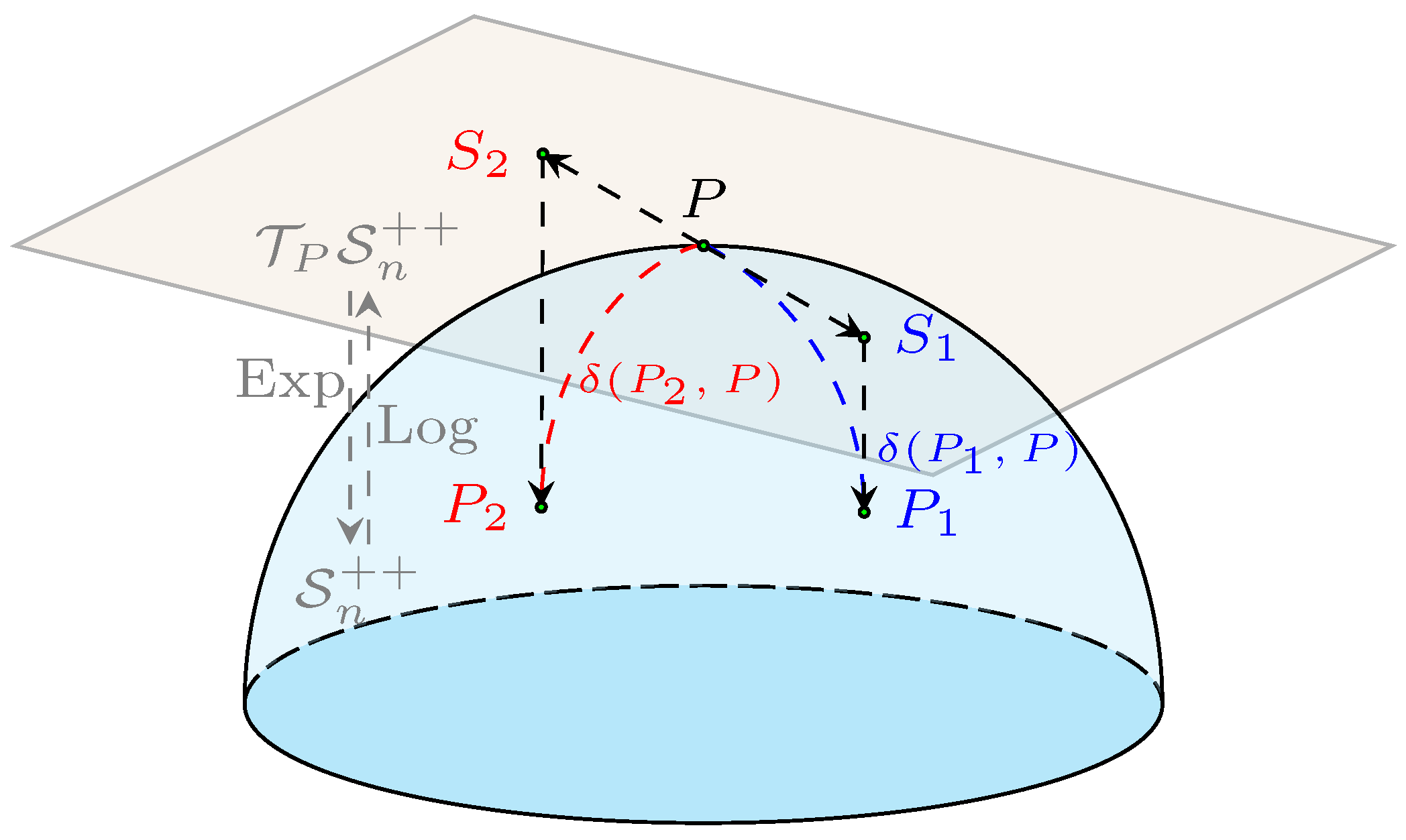
2.1. Geometry of SPD Manifolds

For simplicity, we often replace SPD matrices manifolds with SPD manifolds in the following. The set of $n\times n$ SPD matrices, i.e., real symmetric matrices with strictly positive eigenvalues, is defined as

$$\begin{array}{c}\hfill {\mathcal{S}}_n^{++}=\{P\in {\mathbb{R}}^{n\times n}|P=P^{\top },P\succ 0\}.\end{array}$$

Since ${\mathcal{S}}_n^{++}$ is a differentiable manifold with a natural Riemannian structure [29], some Riemannian geometry tools can be applied to SPD manifolds. The main concept is shown in Figure 1. At any given point $P\in {\mathcal{S}}_n^{++}$, the tangent space, which is the set of all tangent vectors, denoted by ${\mathcal{T}}_P{\mathcal{S}}_n^{++}$, is a symmetric matrix space. The affine-invariant Riemannian metric (AIRM) is one of the most frequently studied Riemannian structures, defined as

$$\begin{array}{c}\hfill \forall A,B\in {\mathcal{T}}_P{\mathcal{S}}_n^{++},{〈A,B〉}_P=\mathrm{tr}\left(P^{-1}A{P}^{-1}B\right).\end{array}$$

The shortest curve connecting two points on the Riemannian manifold is known as a geodesic, and the length of a geodesic is the Riemannian distance. According to AIRM, the Riemannian distance between matrices $P_1,P_2\in {\mathcal{S}}_n^{++}$ is defined as

$$\begin{array}{c}\hfill {\delta }_R(P_1,P_2)={\parallel log\left(P_1^{1/2}{P}_2{P}_1^{1/2}\right)\parallel }_F={\left(\sum _{i=1}^n{log}^2{\lambda }_i\right)}^{1/2},\end{array}$$

(2)

where ${\lambda }_i$ is i-th eigenvalue of $P_1^{1/2}{P}_2{P}_1^{1/2}$. The logarithm of matrix is given by $log\left(P\right)=U\mathrm{diag}(log\left({\sigma }_1\right),\dots ,log\left({\sigma }_n\right))U^{\top }$ in which eigenvalues ${\sigma }_i$ and eigenvector matrix U satisfy $P=U\mathrm{diag}({\sigma }_1,\dots ,{\sigma }_n)U^{\top }$. Similarly, the exponent of matrix is defined as $exp\left(P\right)=U\mathrm{diag}(exp\left({\sigma }_1\right),\dots ,exp\left({\sigma }_n\right))U^{\top }$.

The Riemannian distance is invariant to affine transformations, i.e.,

$$\begin{array}{c}\hfill {\delta }_R\left(P_1,P_2\right)={\delta }_R\left(W^{\top }{P}_{1}W,W^{\top }{P}_{2}W\right),\end{array}$$

(3)

for each W belongs to the general linear group, i.e., $W\in \mathrm{GL}\left(N\right)$. This important affine-invariance property contributes to the robustness of Riemannian BCI decoders [1]. In addition, the affine transformation centres covariance matrices from different sessions or subjects with respect to a reference covariance matrix, making signals comparable, which provides an effective way for transfer learning [30,31].

Similar to the Euclidean geometric mean, the Riemannian mean of given matrices $P_1,\dots ,P_I$ in ${\mathcal{S}}_n^{++}$ is defined as follows:

$$\begin{array}{c}\hfill \overline{P}=\underset{P\in {\mathcal{S}}_n^{++}}{argmin}\sum _{i=1}^I{\delta }_R^2(P,P_i).\end{array}$$

(4)

Several friendly properties of AIRM ensure that $\overline{P}$ exists and is unique while robust to outliers and noise. However, contrary to the Euclidean mean, the Riemannian mean does not have closed-form expression, and efficient iterative algorithms must be employed, such as a fixed point approximation [32]. Minimum distance to Riemannian mean (MDRM) [8], as the name implies, is a simple and parameter-free Riemannian classifier that uses Riemannian distance and mean.

A pair of local projection operators map between SPD matrices on the Riemannian manifold and tangent vectors on the tangent space while preserving geometric information at a given point. More precisely, the logarithmic operator, a mapping from any point $P_i\in {\mathcal{S}}_n^{++}$ to the tangent space at point $P\in {\mathcal{S}}_n^{++}$, i.e., $\mathrm{Log}(·):{\mathcal{S}}_n^{++}\to {\mathcal{T}}_P{\mathcal{S}}_n^{++}$, is defined as

$$\begin{array}{c}\hfill \forall P_i\in {\mathcal{S}}_n^{++},{\mathrm{Log}}_P\left(P_i\right)=S_i=P^{1/2}log(P^{-1/2}{P}_i{P}^{-1/2})P^{1/2}.\end{array}$$

On the contrary, the exponential operator, the inverse map from the tangent vector $S_i\in {\mathcal{T}}_P$ back to the manifold, i.e., $\mathrm{Exp}(·):{\mathcal{T}}_P{\mathcal{S}}_n^{++}\to {\mathcal{S}}_n^{++}$, is also termed the exponential retraction and defined as

$$\begin{array}{c}\hfill \forall S_i\in {\mathcal{T}}_P{\mathcal{S}}_n^{++},{\mathrm{Exp}}_P\left(S_i\right)=P_i=P^{1/2}exp(P^{-1/2}{S}_i{P}^{-1/2})P^{1/2}.\end{array}$$

Consequently, Riemannian distance between points $P,P_i\in {\mathcal{S}}_n^{++}$ can be equivalently defined as Euclidean distance between their tangent vectors.

$$\begin{array}{c}\hfill {\delta }_R(P,P_i)=\parallel {\mathrm{Log}}_P\left(P_i\right){\parallel }_P=\parallel S_i{\parallel }_P=\parallel \mathrm{upper}(P^{-1/2}{\mathrm{Log}}_P\left(P_i\right)P^{-1/2}){\parallel }_2={\parallel s_i-0\parallel }_2,\end{array}$$

(5)

where operator $\mathrm{upper}(·)$ preserves the upper triangular part of the symmetric matrix and vectorizes it with $\sqrt{2}$ weight on the off-diagonal and unity weight elsewhere. Furthermore, $s_i=\mathrm{upper}\left(S_i\right)$ is a $n(n+1)/2$-dimensional vector, where $S_i$ is the tangent vector corresponding to $P_i$.

The above concepts are essential tools for optimization on manifolds [33], whose task is to design efficient algorithms using smooth geometry of the search space. Therefore, simple and efficient Riemannian manifold optimization tools have been developed, such as Manopt (https://www.manopt.org/ (accessed on 1 February 2023)) and Pymanopt (https://pymanopt.github.io/ (accessed on 1 February 2023)). It is worth mentioning that the Python package pyRiemann (https://github.com/alexandrebarachant/pyRiemann (accessed on 1 February 2023)) implements covariance matrix manipulation and signal classification based on Riemannian geometry in BCI.

2.2. Dimensionality Reduction on SPD Manifolds

The purpose of dimensionality reduction on SPD matrices is to learn low-dimensional embedding from original SPD manifolds by a mapping parameterized by W, i.e., $f_W:{\mathcal{S}}_n^{++}\to {\mathcal{S}}_m^{++}(m<n)$. Generally, for a full rank matrix $W\in {\mathbb{R}}^{n\times m}$ and $P\in {\mathcal{S}}_n^{++}$, we have $W^{\top }PW\in {\mathcal{S}}_m^{++}$. In other words, the bilinear mapping preserves the symmetric positive definiteness of the matrices. Therefore, traditional linear mapping for reducing the dimensionality of SPD matrices is defined as

$$\begin{array}{c}\hfill f_W\left(P\right)=W^{\top }PW.\end{array}$$

(6)

Due to the affine invariance of Riemannian distance, the parameter matrix W is usually restricted on the Stiefel manifold, which is denoted as $W\in \mathrm{St}(n,m)$, i.e., $W^{\top }W={\mathit{I}}_m$. The mapping $f_W$ with different parameter W can reflect other intriguing geometry structures of SPD matrices measured by similarity or distance on the low-dimensional manifold. Traditional dimensionality reduction methods for SPD matrices are converted to search for a suitable transformation W, summarized as the following constraint optimization framework:

$$\begin{array}{c}\hfill \underset{W\in \mathrm{St}(n,m)}{min}\mathcal{L}\left(W\right).\end{array}$$

Harandi et al. [17] designed the loss function to maximize discriminative power by exploiting label information and geometric information in the supervised scenario. The affinity function $a(·,·)$ is defined as the difference between within-class similarity and between-class similarity as follows

$$\begin{array}{c}\hfill a(X_i,X_j)=\left\{\begin{array}{cc}1\hfill & X_i\mathrm{and}{X}_j\mathrm{are}\mathrm{adjacent}\mathrm{and}\mathrm{within-class},\hfill \\ -1\hfill & X_i\mathrm{and}{X}_j\mathrm{are}\mathrm{adjacent}\mathrm{and}\mathrm{between-class},\hfill \\ 0\hfill & \mathrm{otherwise},\hfill \end{array}\right.\end{array}$$

thus characterizing the encoding of similarity between SPD matrices. The following objective function is used to achieve discriminative mapping, which means minimizing intra-class distances while maximizing inter-class distances.

$$\begin{array}{c}\hfill \underset{W\in \mathrm{St}(n,m)}{min}\sum _{i,j}a(P_i,P_j){\delta }^2(W^{\top }{P}_{i}W,W^{\top }{P}_{j}W).\end{array}$$

In an unsupervised manner, Horev et al. [18] developed a Riemannian geometry-based PCA formulation by maximizing the Frechet variance of SPD matrices in approximation form as follows.

$$\begin{array}{c}\hfill \underset{W\in \mathrm{St}(n,m)}{max}\sum _i{\delta }^2(W^{\top }{P}_{i}W,W^{\top }\overline{P}W),\end{array}$$

where $\overline{P}$ represents the Riemannian geometric mean as in (4). Another property that has to be mentioned but is not the focus of this article is the non-stationarity of EEG, which is a significant difficulty that BCI online learning needs to overcome. Stationary subspace analysis (SSA) [34,35] deals with the translation problem of covariance through spatial filtering to offset the influence of the signal distribution changing over time. The manifold geometry of SSA [36] is interpreted as mapping the matrix to a separable stationary and non-stationary space, which can be described as variance as follows.

$$\begin{array}{c}\hfill \underset{W\in \mathrm{St}(n,m)}{min}\sum _i{\delta }^2(W^{\top }{\tilde{P}}_{i}W,{\mathit{I}}_m),\end{array}$$

(7)

where ${\tilde{P}}_i={\overline{P}}^{-1/2}{P}_i{\overline{P}}^{-1/2}$ is the pre-whitening matrix with geometric mean $\overline{P}$.

Although those geometry-aware methods for reducing the dimensionality of SPD matrices provide a ground-breaking idea from the viewpoint of Riemannian geometry, the framework relies on the bilinear mapping and loss function, which can only be considered as shallow learning. In this paper, we extend this framework to non-linear mapping by introducing the notion of neural networks in the next section.

3. The Proposed SPD Manifold Network

In this section, we develop a novel non-linear composite mapping to reduce the dimensionality and build the SPD manifolds network (SPD-Mani-Net) on the Siamese architecture to implement deeper metric learning. Figure 2 shows the basic operations of the SPD-Mani-Net.

3.1. SPD-Mani-Net for Reducing Dimensionality

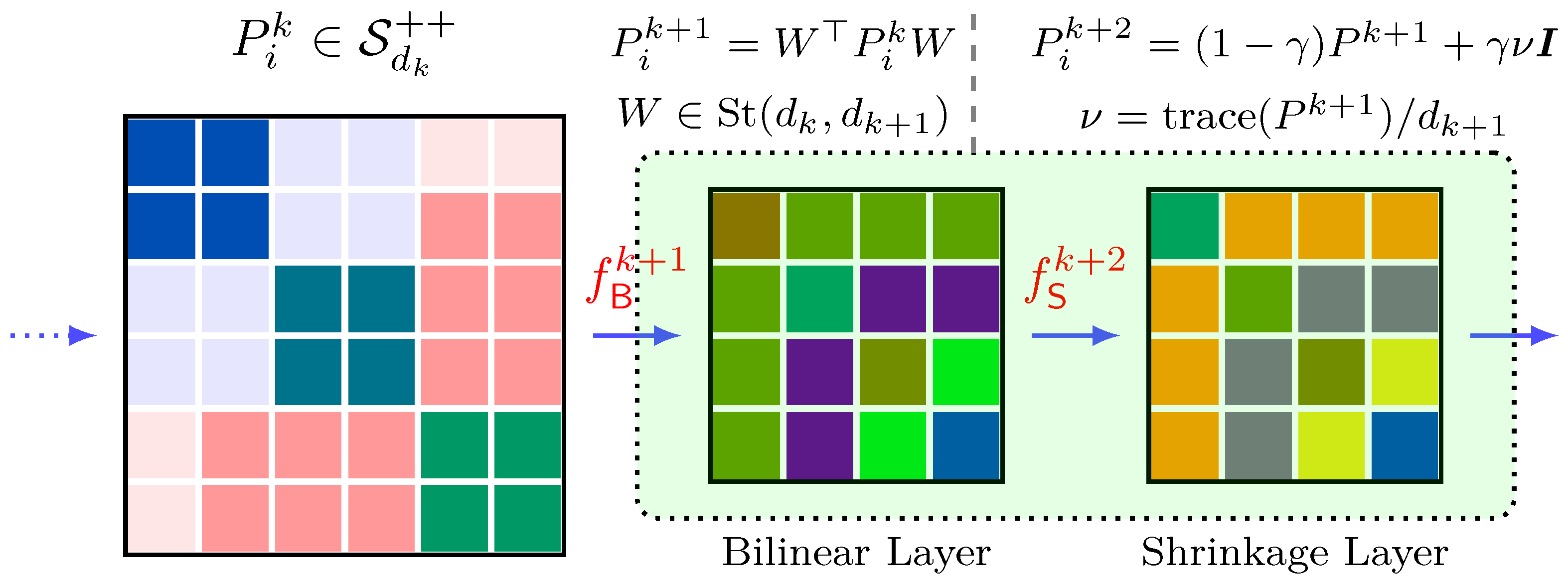
A neural network with K layers can be written as a composition of multiple functions, i.e., $L\circ f^{(K-1)}\circ \dots \circ f^{\left(1\right)}$, where $f^{\left(k\right)}$ corresponds to the function in k-th layer, and final layer usually formalizes its goal as the loss function L. In the SPD-Mani-Net, the previous $K-1$ layers realize the non-linear dimensionality reduction from manifold-to-manifold. The final layer ensures discriminative power on the low-dimensional manifold by a contrastive loss.

Using stochastic gradient descent and backpropagation is typical for training deep networks. Once the errors between the predicted value and ground truth of a mini-batch are obtained in feedforward, we can directly compute the gradient of the loss function of each layer and update model parameters backward, starting from the final layer. The loss function of the k-th layer is denoted as ${\mathcal{L}}^{\left(k\right)}=L\circ f^{(K-1)}\circ \dots \circ f^{\left(k\right)}$, which can be considered intuitively as the error back through the network by $\frac{\partial {\mathcal{L}}^{\left(k+1\right)}\left(P_k,y\right)}{\partial P_k}$. According to the chain rule, the gradient of the function ${\mathcal{L}}^{\left(k\right)}$ in the k-th layer with respect to parameter $W_k$ and input $P_{k-1}$ can be, respectively, calculated by backpropagation:

$$\begin{array}{c}\hfill \begin{array}{cc}\hfill \frac{\partial {\mathcal{L}}^{\left(k\right)}(P_{k-1},y)}{\partial W_k}& =\frac{\partial {\mathcal{L}}^{(k+1)}(P_k,y)}{\partial P_k}\frac{\partial f^{\left(k\right)}\left(P_{k-1}\right)}{\partial W_k},\hfill \\ \hfill \frac{\partial {\mathcal{L}}^{\left(k\right)}(P_{k-1},y)}{\partial P_{k-1}}& =\frac{\partial {\mathcal{L}}^{(k+1)}(P_k,y)}{\partial P_k}\frac{\partial f^{\left(k\right)}\left(P_{k-1}\right)}{\partial P_{k-1}},\hfill \end{array}\end{array}$$

where y is the desired output and $P_k=f^{\left(k\right)}\left(P_{k-1}\right)$ represents the output of the k-th layer of the SPD-Mani-Net. Due to the Stiefel manifold constraint, conventional backpropagation is not suitable for updating $W_k$. For this purpose, we obtain a general backpropagation for each layer to train the SPD-Mani-Net.

Basic layers of SPDNet [26], such as BiMap, ReEig, and LogEig layers, have been widely used in SPD matrix transformation [37,38,39,40,41]. In this paper, we design a novel non-linear shrinkage layer and combine the BiMap to non-linearly reduce the dimensionality of SPD matrices.

3.2. Bilinear Layer

If the k-th layer of the SPD-Mani-Net is bilinear mapping $f_{\mathsf{B}}^{\left(k\right)}$ with input SPD matrix $P_{k-1}\in {\mathcal{S}}_{d_{k-1}}^{++}$, then the low-dimensional output SPD matrix of this layer can be computed as

$$\begin{array}{c}\hfill P_k=f_{\mathsf{B}}^{\left(k\right)}(P_{k-1};W_k)=W_k^{\top }{P}_{k-1}{W}_k,\end{array}$$

where $W_k\in \mathrm{St}(d_{k-1},d_k),(d_k<d_{k-1})$ is the parameter of a k layer network, limited on the Stiefel manifold, so bilinear layer implements dimensionality reduction from $S_{d_{k-1}}^{++}$ to $S_{d_k}^{++}$, i.e., $P_k\in {\mathcal{S}}_{d_k}^{++}$. According to the derivation rule of backpropagation, the Euclidean gradient of the bilinear layer with respect to parameter $W_k^t$, denoted by $\nabla {\mathcal{L}}_{W_k^t}^{\left(k\right)}$, is

$$\begin{array}{c}\hfill \nabla {\mathcal{L}}_{W_k^t}^{\left(k\right)}=2\frac{\partial {\mathcal{L}}^{(k+1)}}{\partial P_k}{\left(W_k^t\right)}^{\top }{P}_{k-1}.\end{array}$$

Since $W_k^t$ is on the Stiefel manifold, the Euclidean gradient $\nabla {\mathcal{L}}_{W_k^t}^{\left(k\right)}$ needs to be converted to the Riemannian gradient $\tilde{\nabla }{\mathcal{L}}_{W_k^t}^{\left(k\right)}$, which involves optimization on the Riemannian manifolds reviewed in the previous section. We refer to [26] for a detailed derivation process of the backpropagation.

$$\begin{array}{c}\hfill \tilde{\nabla }{\mathcal{L}}_{W_k^t}^{\left(k\right)}=\nabla {\mathcal{L}}_{W_k^t}^{\left(k\right)}-\nabla {\mathcal{L}}_{W_k^t}^{\left(k\right)}{W}_k^t{\left(W_k^t\right)}^{\top }.\end{array}$$

In the tangent space, we find a new iteration point $W_k^{t+1}$ by searching along the gradient $\tilde{\nabla }{\mathcal{L}}_{W_k^t}^{\left(k\right)}$, and then project the point back to the Stiefel manifold using the exponential map or a retraction.

$$\begin{array}{c}\hfill {\left(W_k^{t+1}\right)}^{\top }=\Gamma ({(W_k^t)}^{\top }-\lambda \tilde{\nabla }{\mathcal{L}}_{W_k^t}^{\left(k\right)})\end{array}$$

where $\Gamma \left(·\right)$ and $\lambda$ are the retraction operator and learning rate, respectively. The gradient of the bilinear layer with respect to the input $P_{k-1}$ is

$$\begin{array}{c}\hfill \frac{\partial {\mathcal{L}}^{\left(k\right)}(P_{k-1},y)}{\partial P_{k-1}}=\frac{\partial {\mathcal{L}}^{\left(k+1\right)}(P_k,y)}{\partial P_k}{W}_k{W}_k^{\top }.\end{array}$$

3.3. Shrinkage Layer

Although the sample covariance matrix in (1) is an unbiased estimate of the covariance matrix, this estimation from little samples usually becomes imprecise. For high-dimensional data, such as EEG signals, in small training sets, the largest or smallest eigenvalues usually are over- or under-estimated, respectively [42]. The potentially erroneous estimation degrades classification performance. In addition, according to the definition of Riemannian distance in (2), as the dimension increases, the smallest eigenvalues of two SPD matrices tend to zero. It makes the logarithm operator ill-conditioned and unstable. This is the reason why the distance is easily prone to noise. Shrinkage [11,43] is a common approach to compensate for the estimated bias, and covariance matrices are usually replaced by:

$$\begin{array}{c}\hfill \tilde{P}\left(\gamma \right):=(1-\gamma )P+\gamma \nu \mathit{I},\end{array}$$

(8)

where $\gamma \in [0,1]$ is the shrinkage parameter and $\nu$ is defined as the average eigenvalue $\mathrm{tr}\left(P\right)/d$ with dimension of covariance matrix d. After eigenvalue decomposition $P=U\Sigma U^{\top }$, the shrunk covariance matrix in (8) can be rewritten as follows:

$$\begin{array}{c}\hfill \tilde{P}\left(\gamma \right)=(1-\gamma )U\Sigma U+\gamma \nu \mathit{I}=U((1-\gamma )\Sigma +\gamma \nu \mathit{I})U^{\top }.\end{array}$$

It is worth noting that $\tilde{P}$ and P have the same eigenvector matrix U, and $\tilde{P}$ is an SPD matrix with the same dimension of P. More importantly, the extreme eigenvalues of P are modified towards the average value $\nu$, which means that the largest and smallest eigenvalues are shrunk and elongated, respectively. Therefore, proper shrinkage is more effective and robust for small sample training sets. Based on this principle, we design a novel non-linear shrinkage layer to reduce the estimation error of the sample covariance matrix.

If the k-th layer of the SPD-Mani-Net is shrinkage mapping $f_{\mathsf{S}}^{\left(k\right)}$ with the input SPD matrix $P_{k-1}\in {\mathcal{S}}_{d_{k-1}}^{++}$, then output of this layer can be formulated as

$$\begin{array}{c}\hfill P_k=f_{\mathsf{S}}^{\left(k\right)}\left(P_{k-1}\right)=(1-\gamma )P_{k-1}+\gamma \nu \mathit{I}=U_{k-1}((1-\gamma {\Sigma }_{k-1}+\gamma \nu \mathit{I})U_{k-1}^{\top }.\end{array}$$

in which $\gamma$ is a tuning parameter, $\nu$ is the average eigenvalue of the SPD matrix $P_{k-1}$, and $U_{k-1}$, ${\Sigma }_{k-1}$ are the eigenvectors and eigenvalues, respectively, in eigenvalue decomposition: $P_{k-1}=U_{k-1}{\Sigma }_{k-1}{U}_{k-1}^{\top }$. $P_k\in {\mathcal{S}}_{d_{k-1}}^{++}$ means that the shrinkage layer will not change the dimensions of the input SPD matrix.

In addition, the shrinkage layer can effectively shrink eigenvalues of the SPD matrix to the correct estimation meanwhile introducing a non-linear mapping to increase the complexity of dimensionality reduction. Compared with the ReEig layer [26], both can rectify the SPD matrices by tuning their eigenvalues. However, the difference is that the ReEig layer is used to cut off eigenvalues that are less than the rectification threshold $\epsilon$, i.e., $max(\epsilon \mathit{I},{\Sigma }_{k-1})$, while the shrinkage layer shrinks all eigenvalues towards the weighted spherical covariance matrix, to decrease a systematic bias due to a small sample set. So, the shrinkage layer is to the ReEig layer what soft thresholding is to hard thresholding.

As shown in [26], since the parameter $\gamma$ in the shrinkage layer is fixed, we compute the gradient of loss ${\mathcal{L}}^{\left(k\right)}$ with respect to input $P_{k-1}$ by the chain rule of matrix backpropagation.

$$\begin{array}{c}\hfill \frac{\partial {\mathcal{L}}^{\left(k\right)}}{\partial P_{k-1}}=U\left(2M^{\top }\circ {\left(U^{\top }\frac{\partial {\mathcal{L}}^{\left(k^{\prime }\right)}}{\partial U}\right)}_{\mathrm{sym}}+{\left(\frac{\partial {\mathcal{L}}^{\left(k^{\prime }\right)}}{\partial \Sigma }\right)}_{\mathrm{diag}}\right)U^{\top },\end{array}$$

where $M\left(i,j\right)=\left\{\begin{array}{cc}\frac{1}{{\sigma }_i-{\sigma }_j},\hfill & i\ne j\hfill \\ 0,\hfill & i=j\hfill \end{array}\right.$, ${(·)}_{\mathrm{sym}}$ and ${(·)}_{\mathrm{diag}}$ represent symmetric and diagonal operators, respectively. Because the shrinkage layer involves an eigenvalue decomposition, we introduce a virtual layer ($k^{\prime }$-th layer) for this operation. Due to $\mathrm{d}{P}_k=2{\left(\mathrm{d}U(\left(1-\gamma \right)\Sigma +\gamma \nu \mathit{I})U^{\top }\right)}_{\mathrm{sym}}+{\left(U\left(1-\gamma \right)\mathrm{d}\Sigma U^{\top }\right)}_{\mathrm{sym}}$, we compute two partial derivatives as follows:

$$\begin{array}{c}\hfill \begin{array}{cc}\hfill \frac{\partial {\mathcal{L}}^{\left(k^{\prime }\right)}}{\partial U}& =2{\left(\frac{\partial {\mathcal{L}}^{\left(k+1\right)}}{\partial P_k}\right)}_{\mathrm{sym}}U((1-\gamma )\Sigma +\gamma \nu \mathit{I})\hfill \\ \hfill \frac{\partial {\mathcal{L}}^{\left(k^{\prime }\right)}}{\partial \Sigma }& =(1-\gamma )U^{\top }{\left(\frac{\partial {\mathcal{L}}^{(k+1)}}{\partial P_k}\right)}_{\mathrm{sym}}U.\hfill \end{array}\end{array}$$

To date, we propose two types of layers of the SPD-Mani-Net: a bilinear mapping layer for dimensionality reduction and a non-linear shrinkage layer for correcting eigenvalues. Furthermore, we also deduce the backpropagation of these layers to train the network.

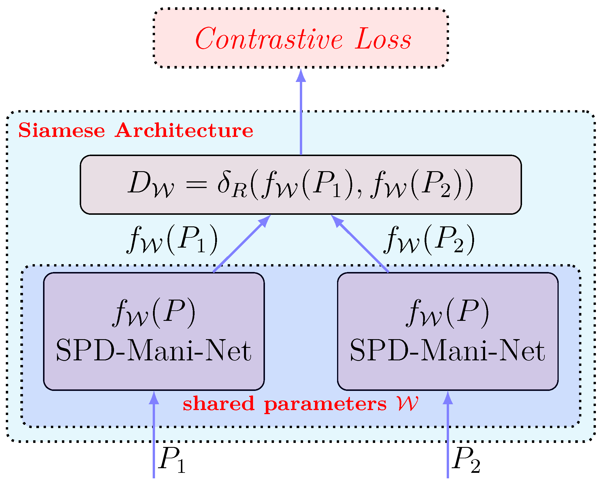
3.4. Siamese Architecture for Discriminative Learning

Considering the purpose of dimensionality reduction for SPD manifolds, we extend traditional linear dimensionality reduction mapping to the non-linear transformation, i.e., the previous $K-1$ layers of the SPD-Mani-Net denoted as $f_{\mathcal{W}}$. As shown in Figure 3, we aim to make $f_{\mathcal{W}}$ more discriminative by Siamese architecture to perform distance metric learning.

In the Siamese network, we input a pair of high-dimensional SPD matrices $P_1^i$ and $P_2^i$ and obtain the corresponding low-dimensional SPD matrices $f_{\mathcal{W}}\left(P_1^i\right)$ and $f_{\mathcal{W}}\left(P_2^i\right)$ through $f_{\mathcal{W}}$ with shared parameters $\mathcal{W}$. The Riemannian distance between $f_{\mathcal{W}}\left(P_1^i\right)$ and $f_{\mathcal{W}}\left(P_2^i\right)$, i.e., $D_{\mathcal{W}}^i={\delta }_R(f_{\mathcal{W}}\left(P_1^i\right),f_{\mathcal{W}}\left(P_2^i\right))$, provides a set of neighbourhood relationships on the low-dimensional manifold. Therefore, similarity metrics can be measured by Riemannian distance. Let Y be a binary label for this pair of SPD matrices. If $P_1^i$ and $P_2^i$ are similar, $Y=0$. Otherwise, $Y=1$. For low-dimensional embeddings, the final layer of the SPD-Mani-Net minimizes the contrast loss function by reducing the distance between covariance matrices of similar signals pairs while increasing the distance between dissimilar pairs:

$$\begin{array}{c}\hfill L\left(\mathcal{W}\right)=\sum _{i=1}^P\frac{1-Y^i}{2}{\left(D_{\mathcal{W}}^i\right)}^2+\frac{Y^i}{2}{(max(0,m-D_{\mathcal{W}}^i))}^2,\end{array}$$

where $m>0$ in the second item is a margin, which enforces the pair of dissimilar points pushed apart if the distance is less than m. Instead, they are unaffected if the distance is more than m. Moreover, the first item attracts all pairs of similar points on the manifold. By training the SPD-Mani-Net, all points on the low-dimensional SPD manifold will be in equilibrium. Thus, we can make the low-dimensional SPD manifold more separable. The gradient of contrast loss function with respect to the parameters $\mathcal{W}$ can be calculated by backpropagation in the SPD-Mani-Net.

$$\begin{array}{c}\hfill \frac{\partial L\left(\mathcal{W}\right)}{\partial \mathcal{W}}=\sum _{i=1}^P\frac{\partial D_{\mathcal{W}}^i}{\partial \mathcal{W}}((1-Y^i)D_{\mathcal{W}}^i+Y^{i}max(0,m-D_{\mathcal{W}}^i)).\end{array}$$

(9)

As can be seen from the above equation, due to the sharing of parameters between the two same branches of the Siamese network, the gradient is the sum of contributions from $f_{\mathcal{W}}\left(P_1^i\right)$ and $f_{\mathcal{W}}\left(P_2^i\right)$. For $k=1,2$, we have

$$\begin{array}{c}\hfill \frac{\partial L\left(\mathcal{W}\right)}{\partial f_{\mathcal{W}}\left(P_k^i\right)}=\frac{\partial D_{\mathcal{W}}^i}{\partial f_{\mathcal{W}}\left(P_k^i\right)}\left(\left(1-Y^i\right)D_{\mathcal{W}}^i+Y^{i}max\left(0,m-D_{\mathcal{W}}^i\right)\right).\end{array}$$

More details to derive $\frac{\partial D_{\mathcal{W}}^i}{\partial f_{\mathcal{W}}\left(P_k^i\right)}$ can be found in Appendix A.

The proposed SPD-Mani-Net uses the Siamese architecture to make the non-linear dimensionality reduction mapping more discriminative. After mapping, the covariance matrices are still on low-dimensional manifolds instead of Euclidean vectors, which is another difference between the SPD-Mani-Net and SPD-Net [26].

4. Transfer Learning

It is essential to know that signals of different sessions or subjects are well separated on the original manifold. However, cross-session or cross-subject classification is not a tractable problem. Since the methods above are suitable only for an individual subject to obtain an appropriate low-dimensional embedding, applying the mapping to other subjects usually results in poor performance. Therefore, the subject-to-subject transfer learning can effectively reduce the calibration time of the BCI and ensure the mapping is valid for other subjects [44]. The affine-invariance property of the Riemannian distance in (3) makes it possible for transfer learning by a reference covariance matrix [30]. In addition, the Riemannian framework is more robust to modifications of spatial distributions, providing a good cross-subject and across-session generalization capability [1,45].

In [43,46], a regularization method based on Riemannian geometry was proposed to obtain a more robust estimation of the covariances matrices, which can improve performance, especially in a small sample set. The Riemannian distance was used to measure the geometric information of covariance matrices between the target subject and other subjects. Thus, the composite covariance matrices can be estimated by regularizing the target subject covariance matrices towards similar subjects.

This idea of reusing covariance matrices from other subjects motivates us to design a regularization (Reg) layer to perform subject-to-subject transfer learning to improve the SPD-Mani-Net. Here, a network combined with transfer regularization is abbreviated as SPD-Mani-Net+Reg. An illustration of the regularization layer is shown in Figure 4.

To be more precise, according to the affine-invariance property, we move the target subject’s original mean of covariance matrices to the composite covariance matrix. The transformation retains geometric information for the individual subject and makes the transformed covariance matrices comparable for all subjects. We use bilinear mapping to perform this transformation.

$$\begin{array}{c}\hfill {\tilde{P}}_k^i=W_k^{\top }{P}_k^i{W}_k,\end{array}$$

where $P_k^i$ denotes the i-th covariance matrix of the k-th subject, ${\tilde{P}}_k^i$ is the transformed matrix corresponding to $P_k^i$. Furthermore, the transformation $W_k$ is invertible. Hence, we can easily obtain the relationship between the original mean ${\overline{P}}_k$ of covariance matrices and transformed mean ${\widehat{P}}_k$ for the k-th subject.

$$\begin{array}{c}\hfill {\widehat{P}}_k=W_k^{\top }{\overline{P}}_k{W}_k.\end{array}$$

(10)

Our goal is to obtain the transformation $W_k$ from ${\overline{P}}_k$ to the target matrix ${\widehat{P}}_k$. Obviously, both ${\overline{P}}_k$ and ${\widehat{P}}_k$ are SPD matrices, an alternative solution is given by

$$\begin{array}{c}\hfill W_k={\overline{P}}_k^{-1/2}{\left({\overline{P}}_k^{1/2}{\widehat{P}}_k{\overline{P}}_k^{1/2}\right)}^{1/2}{\overline{P}}_k^{-1/2}.\end{array}$$

In particular, if we set target matrix ${\widehat{P}}_k$ to the identity the matrix as was performed in [30], the transformation $W_k={{\overline{P}}_k}^{1/2}$. We propose to regularize covariance matrices in the estimation of the target matrices ${\widehat{P}}_k$:

$$\begin{array}{c}\hfill {\widehat{P}}_k=\left(1-\lambda \right){\overline{P}}_k+\lambda \sum _{i\ne k}\frac{1}{{\gamma }_i}{\overline{P}}_i,\end{array}$$

where ${\gamma }_i=\frac{{\delta }_R({\overline{P}}_k,{\overline{P}}_i)}{{\sum }_j{\delta }_R({\overline{P}}_k,{\overline{P}}_j)}$ is the normalized weight, and $\lambda \in [0,1]$ is the regularization parameter. Similar to the shrinkage layer, the Reg layer is essentially a linear combination of the original matrix and the reference matrix, which guides the estimates towards well-estimated covariance matrices. ${\widehat{P}}_k\in {\mathcal{S}}_{d_m}^{++}$ means that the composite covariance matrices for the target subject are a weighted average of the covariance matrices of all subjects to make the matrices comparable on the original manifold.

5. Experiments

To evaluate the performance of the proposed SPD-Mani-Net, we performed experiments on both toy data and EEG signal datasets in BCI, respectively.

5.1. Toy Data

We randomly generate toy data $\Lambda =\left\{{\Lambda }_i\in {\mathcal{S}}_n^{++}\right\}$ of 400 SPD matrices with four labels, where the dataset contains 200 training samples and 200 test samples. The inherent dimension of the structure is $m=10$, and the actual dimension of the structure is $n=30$. A brief generation scheme used in [47] is as follows: The high-dimensional data consists of two parts: inherent feature vector $s_i^{\mathrm{fea}}\in {\mathbb{R}}^{m(m+1)/2}$ and auxiliary vector $s_i^{\mathrm{aug}}\in {\mathbb{R}}^{n(n+1)/2-m(m+1)/2}$, where $s_i^{\mathrm{fea}}=m_0+0.5m_k+n_i^{\mathrm{fea}}$. Here, $m_0,m_k\sim U{\left(0,1\right)}^{m(m+1)/2}$ and $n_i^{\mathrm{fea}}\sim {\mathcal{N}}_{m(m+1)/2}(0,{\sigma }^2)$ represent the overall data centre, the deviation between the centre of the k-th class samples and $m_0$ and individual information used to distinguish for each sample, respectively. Furthermore, $s_i^{\mathrm{aug}}\sim {\mathcal{N}}_{n(n+1)/2-m(m+1)/2}\left(0,{\delta }^2\right)$ increases the dimension of the inherent structure. As $\sigma$ and $\delta$ increase, the toy data are more difficult to classify. The resulting high-dimensional vector can be expressed as $s_i={\left[\begin{array}{cc}{\left(s_i^{\mathrm{fea}}\right)}^{\top }& {\left(s_i^{\mathrm{aug}}\right)}^{\top }\end{array}\right]}^{\top }\in {\mathbb{R}}^{n(n+1)/2}$ and projected onto the manifold by the inverse mapping of the operator $\mathrm{upper}(·)$ in (5) to obtain the corresponding SPD matrix ${\Lambda }_i$. Here, we validate our algorithm in the different parameter settings: feature distribution $\sigma =0.1,0.3,0.5$ and noise variance $\delta =0.1,0.3,0.5$.

We compare the proposed algorithm with the following algorithms. The SPD matrices obtained by all dimensionality reduction algorithms are classified by the MDRM [8] algorithm. For the comparison criteria, we choose classification accuracy to measure the discriminative power of the manifold.

• Ga-DR [17]: a linear method based on metric learning.
• Ga-PCA [18]: a linear method based on variance maximizing.
• DPLM [19]: a linear method based on distance preservation to local mean.
• SPD-Net [26]: a non-linear method based on the SPD-Net, including BiMap and ReEig layers.
• SPD-Mani-Net: A non-linear method based on the SPD-Mani-Net, including BiMap and shrinkage layers, as shown in Figure 3.

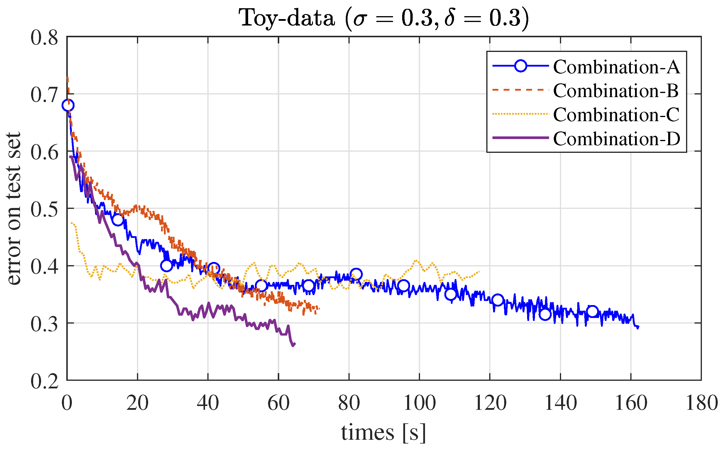
As for the toy data, we reduce the dimensionality of manifolds from their original size $n=30$ to the target size $m=10$ in all algorithms. We apply the same Riemannian metric and neighbour parameters setting as described in [19] for traditional linear dimensionality reduction methods Ga-DR, Ga-PCA, and DPLM. For non-linear dimensionality reduction methods, SPD-Net and SPD-Mani-Net have the same layers, which include three BiMap layers and two non-linear mapping layers. The differences between the two networks are structure and non-linear mapping. The sizes of transformation parameters in BiMap layers are set to $30\times 25$, $25\times 20$, and $20\times 10$, respectively. Other parameters are set as recommended in the SPD-Net [26]. We fix learning rate $\lambda ={10}^{-2}$ and all thresholds in ReEig layers $\epsilon ={10}^{-4}$. We set the batch size to 50 and initialized parameters in BiMap layers to random semi-orthogonal matrices. In shrinkage layers, the parameters $\gamma$ are set to 0.01.

As can be seen from

Table 1. Recognition accuracy for toy data.

Method		Accuracy
	$\mathit{\sigma }$	0.1	0.1	0.1	0.3	0.3	0.3	0.5	0.5	0.5
	$\mathit{\delta }$	0.1	0.3	0.5	0.1	0.3	0.5	0.1	0.3	0.5
Ga-DR [17]		100%	91%	40%	84%	62.5%	32.5%	53.5%	48.5%	34.5%
Ga-PCA [18]		73%	87%	52.5%	60.5%	38%	34%	44%	36%	28%
DPLM [19]		100%	56.5%	33%	84.5%	47.5%	26%	47.5%	59%	32%
SPD-Net [26]		100%	89.5%	52%	87.5%	69%	47.5%	63.5%	56%	41.5%
SPD-Mani-Net		100%	99%	84%	89%	67.5%	54.5%	64%	65%	51.5%

, on the randomly generated toy data, as $\sigma$ and $\delta$ increase, non-linear methods SPD-net and SPD-Mani-Net is better than linear methods Ga-DR, Ga-PCA and DPLM. It indicates that non-linear layers improve dimensionality reduction performance by tuning the eigenvalues of the SPD matrices. The result that our approach achieves better accuracy in almost all cases and illustrates the SPD-Mani-Net is superior to other methods with respect to noise robustness. In addition, the SPD-Mani-Net can be regarded as a non-linear extension of Ga-DR, which performs deeper metric learning.

5.2. Ablation Study

To explore the impact of the shrinkage layer and Siamese architecture on performance improvement, we set up four groups of comparative experiments by controlling factors in

Table 2. The configuration of combinations.

	Shrinkage Layer	Siamese Architecture	Type
Combination A			SPD-Net
Combination B	✓		SPD-Net
Combination C		✓	SPD-Mani-Net
Combination D	✓	✓	SPD-Mani-Net

. Combination A uses the ReEig layer instead of the shrinkage layer and vice versa for combination B. We tested on toy data with $\sigma =\delta =0.3$, and results are shown in Figure 5.

Compared with the ReEig layer, it can be seen that the shrinkage layer does not improve the classification accuracy significantly but shorten the training time, which is due to the fact that the forward propagation does not require SVD. According to the curve of combination D, the Siamese architecture is the main factor in improving the reducing classification error.

5.3. EEG Signals from Motor Image BCIs

In the case of real datasets, we used EEG data from two publicly available datasets of BCI competitions to evaluate the SPD-Mani-Net. The major configurations of the datasets that contain motor imagery (MI) EEG signals are shown in

Table 3. The configuration of competition data.

	IIIa of Competition III	IIa of Competition IV
Number of subjects	3	9
Number of channels	60	22
Number of classes	4	4
Trials per class	60	144
Sampling rate	250 Hz	250 Hz
Filter Bank	bandpass 8–30 Hz	bandpass 8–30 Hz

. As was performed in [45], only signals of the left- and right-hand MI trials were used for classification on the two-class problem.

• Dataset IIIa, BCI competition III [48]: This dataset includes EEG signals from 60 channels and 3 subjects, who performed four types of tasks (left-hand, right-hand, foot, and tongue MI). In this experiment, only EEG signals corresponding to left- and right-hand MI were used for the present study. Training and testing sets were available for each subject. Both sets contain 45 trials for B1 and 30 trials per class for B2 and B3.
• Dataset IIa, BCI competition IV [49]: This dataset contains EEG signals consisting of 22 channels from 9 subjects, who performed four types of the same tasks as the last dataset. We also selected signals of left- and right-hand MI trials to enable a proper comparison. Training and testing sets were available for each subject, containing 72 trials per class from C1 to C9.

We carried out the same pre-processing for each dataset and trial as performed in [45]. In addition to the above six dimensionality reduction methods used in the toy data, we also compared the MDRM classification method [8] on the original manifolds, and the well-known spatial filter CSP [2] used to extract features in BCI as a reference.

The dimension of manifolds reduced from the original size to the target size $m=6$ in both datasets. For linear methods, the metric and neighbour parameters are set up as recommended in [19]. For non-linear methods, we still construct the same structure of the SPD-Net and SPD-Mani-Net, which include five BiMap layers and five non-linear mapping layers. In the former dataset, the sizes of the transformation parameters in BiMap layers are set to $60\times 50$, $50\times 40$, $40\times 30$, $30\times 20$, and $20\times 6$, respectively. In the latter dataset, we configure sizes to $22\times 19$, $19\times 16$, $16\times 13$, $13\times 10$, and $10\times 6$, respectively. We fix the learning rate $\lambda ={10}^{-2}$ and all thresholds in the ReEig layers $\epsilon ={10}^{-4}$. We chose a batch size of 50 and initialized parameters in BiMap layers to random semi-orthogonal matrices. In the shrinkage layers, all shrinkage parameters $\gamma$ are set to 0.1.

The accuracy of the classification is presented in

Table 4. Classification accuracies for the EEG datasets from motor image BCIs.

Accuracy	Mean ± Std	BCI Competition III Dataset IIIa			BCI Competition IV Dataset IIa
Subject		B1	B2	B3	C1	C2	C3	C4	C5	C6	C7	C8	C9
MDRM [8]	78.5 ± 16.1	97.8	63.3	88.3	88.2	52.8	92.4	71.5	58.3	64.6	75	95.8	94.4
CSP+LDA [2]	79.4 ± 16.8	95.6	61.7	93.3	88.9	51.4	96.5	70.1	54.9	71.5	81.3	93.8	93.8
Ga-DR [17]	78.2 ± 14.9	96.7	68.3	85	87.5	53.5	92.4	73.6	57.6	68.0	70.8	94.4	91.6
Ga-PCA [18]	68.5 ± 13.0	80	63.3	68.3	77.8	50	84.7	64.5	53.4	56.9	56.2	84.0	84.0
DPLM [19]	75.6 ± 15.3	85.6	63.3	75	89.6	56.9	93.1	70.8	56.9	58.3	68.0	95.1	94.4
SPD-Net [26]	76.9 ± 17.1	97.7	66.7	88.3	84.7	56.3	93.8	68.1	56.9	62.5	56.3	95.8	95.1
SPD-Mani-Net	83.1 ± 14.9	100	66.7	98.3	94.4	57.6	93.1	75	71.5	66.7	83.3	96.5	94.4

. As can be seen, the SPD-Mani-Net achieves the highest mean accuracies, showing that the SPD-Mani-Net outperforms other methods for most subjects. The improved performance of the SPD-Mani-Net can be attributed to two factors: A non-linear network for dimensionality reduction and Siamese architecture for metric learning. By comparing the Ga-DR and SPD-Mani-Net, we know that introducing non-linear mapping can improve the performance of metric learning. Because the LogEig layer in the SPD-Net vectorizes the SPD matrices, and the vectors are then fed into the Euclidean network, the result of the SPD-Net is not ideal in this experiment.

5.4. EEG Signals from Motor Image Multi-Subject BCIs

To evaluate how the Reg layer can improve the performance of the SPD-Mani-Net, we compare several methods on two EEG signal datasets: MDRM on the original manifolds, SPD-Net, SPD-Mani-Net, and SPD-Mani-Net with Reg layer, called the SPD-Mani-Net+Reg for simplicity. In this experiment, we select all signals of four motor imagery tasks, i.e., right-hand, left-hand, foot, and tongue. In addition, we merge all signals of each subject as the training and testing set for each dataset.

The parameters and pre-processing of this experiment are generally the same as the previous experiment. In the SPD-Net and SPD-Mani-Net, there are two BiMap layers and two shrinkage layers. We configure sizes of transformation parameters in the BiMap layers to $22\times 15$, $15\times 10$ for Dataset IIa of BCI competition IV and $60\times 40$, $40\times 10$ for Dataset IIIa of BCI competition III, respectively. The shrinkage parameters $\gamma =0.01$ and the parameter in the Reg layer $\lambda =0.1$.

In addition to classification accuracy, we also use the Kappa coefficient to measure the performance of different dimensionality reduction methods on the multi-class case. The Kappa coefficient is calculated from the confusion matrix C. Firstly, we compute the overall accuracy $p_0=\frac{1}{N}{\sum }_{i=1}^M{c}_{ii}$, where $c_{ii}$ is the i-th diagonal element of the confusion matrix C. M and N indicate the number of signal classes and samples, respectively. Then we can compute the chance probability $p_e=\frac{1}{N^2}{\sum }_{i=1}^M{c}_{:i}{c}_{i:}$, where $c_{:i}$ and $c_{i:}$ represent the sum of the i-th row and i-th column of the confusion matrix C, respectively. The Kappa coefficient is calculated as $\kappa =\frac{p_0-p_e}{1-p_e}\in (0,1)$. The closer the Kappa coefficient is to 1, the higher the consistency of predicted results with actual labels.

The performance of classifications is compared in terms of accuracy and Kappa coefficient in

Table 5. Classification accuracies for the EEG datasets from motor image multi-subject BCIs.

Accuracy	Mean ± Std	BCI Competition III Dataset IIIa			BCI Competition IV Dataset IIa
Subject		B1	B2	B3	C1	C2	C3	C4	C5	C6	C7	C8	C9
MDRM [8]	43.61 ± 16.71	67.78	39.17	27.50	61.46	27.08	64.93	39.93	25.00	22.22	61.46	46.88	39.93
SPD-Net [26]	45.75 ± 17.56	70.56	36.67	38.33	66.67	26.74	69.80	37.50	25.35	26.04	55.21	60.07	36.11
SPD-Mani-Net	48.21 ± 15.73	65.00	33.33	35.00	65.28	28.13	68.75	45.49	29.51	34.03	51.74	64.58	57.64
SPD-Mani-Net+Reg	53.28 ± 17.78	83.30	43.30	32.50	61.11	33.33	69.44	42.71	39.24	32.99	62.85	69.44	69.10

and

Table 6. Kappa coefficient for the EEG datasets from motor image multi-subject BCIs.

Kappa	Mean ± Std	BCI Competition III Dataset IIIa			BCI Competition IV Dataset IIa
Subject		B1	B2	B3	C1	C2	C3	C4	C5	C6	C7	C8	C9
MDRM [8]	0.25 ± 0.22	0.57	0.19	0.03	0.49	0.02	0.53	0.20	0.00	0.00	0.49	0.29	0.20
SPD-Net [26]	0.28 ± 0.24	0.61	0.16	0.18	0.56	0.02	0.60	0.17	0.00	0.01	0.40	0.47	0.15
SPD-Mani-Net	0.31 ± 0.21	0.53	0.11	0.13	0.54	0.04	0.58	0.27	0.06	0.12	0.35	0.53	0.44
SPD-Mani-Net+Reg	0.37 ± 0.24	0.78	0.24	0.10	0.48	0.11	0.59	0.23	0.18	0.10	0.50	0.59	0.58

. The performance of the three non-linear methods can be improved to varying degrees. In particular, compared with the SPD-Mani-Net, the accuracies and Kappa coefficients on the low-dimensional manifolds obtained by the SPD-Mani-Net+Reg are significantly improved for most subjects, which demonstrates that the Reg layer can effectively perform transfer. Overall, the SPD-Mani-Net+Reg can improve the level of performance for bad subjects, which means the subjects with lower accuracy on the original manifolds, such as C5 and C9.

6. Conclusions

In this paper, we explored neural networks to reduce the dimensionality of SPD covariance matrices such that the low-dimensional manifold becomes more discriminative. To that end, a manifold network consisting of traditional bilinear layers and novel non-linear shrinkage layers was established on the Siamese architecture for deep metric learning from manifold-to-manifold. Furthermore, a regularization layer was designed to perform subject-to-subject transfer learning for multi-subject BCI. Numerical experiments on toy data showed that shrinkage layers are robust to noise. Furthermore, the experimental results on EEG datasets demonstrate the efficiency of the proposed SPD-Mani-Net. Moreover, the results of transfer learning indicate that the proper regularization layer makes the data more interpretable.

Our future work will focus on improving and deepening the proposed network by effectual network structure, such as Triplet network, and efficient network training tricks, such as network regularization and data augmentation. In addition, new developments in other fields may bring new opportunities, such as the concept of causality and mind-light-matter [50]. In practical applications, the non-stationarity not considered in this paper motivates us to design a new regularization layer from the model (7) to realize signal pre-processing, which provides a possible solution for the online learning of BCI.

References

1. Congedo, M.; Barachant, A.; Bhatia, R. Riemannian geometry for EEG-based brain–computer interfaces; a primer and a review. Brain Comput. Interfaces 2017, 4, 155–174. [Google Scholar] [CrossRef]
2. Blankertz, B.; Tomioka, R.; Lemm, S.; Kawanabe, M.; Muller, K.R. Optimizing spatial filters for robust EEG single-trial analysis. IEEE Signal Process. Mag. 2007, 25, 41–56. [Google Scholar] [CrossRef]
3. Lotte, F.; Congedo, M.; Lécuyer, A.; Lamarche, F.; Arnaldi, B. A review of classification algorithms for EEG-based brain–computer interfaces. J. Neural Eng. 2007, 4, R1. [Google Scholar] [CrossRef] [PubMed] [Green Version]
4. Yger, F.; Berar, M.; Lotte, F. Riemannian approaches in brain–computer interfaces: A review. IEEE Trans. Neural Syst. Rehabil. Eng. 2016, 25, 1753–1762. [Google Scholar] [CrossRef] [PubMed] [Green Version]
5. Lotte, F.; Bougrain, L.; Cichocki, A.; Clerc, M.; Congedo, M.; Rakotomamonjy, A.; Yger, F. A review of classification algorithms for EEG-based brain–computer interfaces: A 10 year update. J. Neural Eng. 2018, 15, 031005. [Google Scholar] [CrossRef] [Green Version]
6. Liu, X.; Liu, S.; Ma, Z. A Framework for Short Video Recognition Based on Motion Estimation and Feature Curves on SPD Manifolds. Appl. Sci. 2022, 12, 4669. [Google Scholar] [CrossRef]
7. Tuzel, O.; Porikli, F.; Meer, P. Pedestrian detection via classification on riemannian manifolds. IEEE Trans. Pattern Anal. Mach. Intell. 2008, 30, 1713–1727. [Google Scholar] [CrossRef]
8. Barachant, A.; Bonnet, S.; Congedo, M.; Jutten, C. Multiclass brain–computer interface classification by Riemannian geometry. IEEE Trans. Biomed. Eng. 2011, 59, 920–928. [Google Scholar] [CrossRef] [Green Version]
9. Wu, D.; Lance, B.J.; Lawhern, V.J.; Gordon, S.; Jung, T.P.; Lin, C.T. EEG-based user reaction time estimation using Riemannian geometry features. IEEE Trans. Neural Syst. Rehabil. Eng. 2017, 25, 2157–2168. [Google Scholar] [CrossRef] [Green Version]
10. Gao, W.; Ma, Z.; Gan, W.; Liu, S. Dimensionality reduction of SPD data based on riemannian manifold tangent spaces and isometry. Entropy 2021, 23, 1117. [Google Scholar] [CrossRef]
11. Ledoit, O.; Wolf, M. A well-conditioned estimator for large-dimensional covariance matrices. J. Multivar. Anal. 2004, 88, 365–411. [Google Scholar] [CrossRef] [Green Version]
12. Tenenbaum, J.B.; Silva, V.d.; Langford, J.C. A global geometric framework for nonlinear dimensionality reduction. Science 2000, 290, 2319–2323. [Google Scholar] [CrossRef] [PubMed]
13. Roweis, S.T.; Saul, L.K. Nonlinear dimensionality reduction by locally linear embedding. Science 2000, 290, 2323–2326. [Google Scholar] [CrossRef] [PubMed] [Green Version]
14. Förstner, W.; Moonen, B. A metric for covariance matrices. In Geodesy-the Challenge of the 3rd Millennium; Springer: Berlin/Heidelberg, Germany, 2003; pp. 299–309. [Google Scholar]
15. Xie, X.; Yu, Z.L.; Lu, H.; Gu, Z.; Li, Y. Motor imagery classification based on bilinear sub-manifold learning of symmetric positive-definite matrices. IEEE Trans. Neural Syst. Rehabil. Eng. 2016, 25, 504–516. [Google Scholar] [CrossRef] [Green Version]
16. Li, Y.; Lu, R. Locality preserving projection on SPD matrix Lie group: Algorithm and analysis. Sci. China-Inf. Sci. 2018, 61, 092104. [Google Scholar] [CrossRef] [Green Version]
17. Harandi, M.; Salzmann, M.; Hartley, R. Dimensionality reduction on SPD manifolds: The emergence of geometry-aware methods. IEEE Trans. Pattern Anal. Mach. Intell. 2017, 40, 48–62. [Google Scholar] [CrossRef] [Green Version]
18. Horev, I.; Yger, F.; Sugiyama, M. Geometry-aware principal component analysis for symmetric positive definite matrices. Mach. Learn. 2017, 106, 493–522. [Google Scholar] [CrossRef] [Green Version]
19. Davoudi, A.; Ghidary, S.S.; Sadatnejad, K. Dimensionality reduction based on distance preservation to local mean for symmetric positive definite matrices and its application in brain–computer interfaces. J. Neural Eng. 2017, 14, 036019. [Google Scholar] [CrossRef] [Green Version]
20. Feng, S.; Hua, X.; Zhu, X. Matrix information geometry for spectral-based SPD matrix signal detection with dimensionality reduction. Entropy 2020, 22, 914. [Google Scholar] [CrossRef]
21. Popović, B.; Janev, M.; Krstanović, L.; Simić, N.; Delić, V. Measure of Similarity between GMMs Based on Geometry-Aware Dimensionality Reduction. Mathematics 2022, 11, 175. [Google Scholar] [CrossRef]
22. Chopra, S.; Hadsell, R.; LeCun, Y. Learning a similarity metric discriminatively, with application to face verification. Proc. IEEE Comput. Soc. Conf. Comput. 2005, 1, 539–546. [Google Scholar]
23. Hadsell, R.; Chopra, S.; LeCun, Y. Dimensionality reduction by learning an invariant mapping. Proc. IEEE Comput. Soc. Conf. Comput. 2006, 2, 1735–1742. [Google Scholar]
24. Hoffer, E.; Ailon, N. Deep metric learning using triplet network. In Proceedings of the Similarity-Based Pattern Recognition: Third International Workshop, SIMBAD 2015, Copenhagen, Denmark, 12–14 October 2015; Springer: Berlin/Heidelberg, Germany, 2015; pp. 84–92. [Google Scholar]
25. Schroff, F.; Kalenichenko, D.; Philbin, J. Facenet: A unified embedding for face recognition and clustering. In Proceedings of the IEEE Conference on Computer Vision and Pattern Recognition, Boston, MA, USA, 7–12 June 2015; pp. 815–823. [Google Scholar]
26. Huang, Z.; Van Gool, L. A riemannian network for spd matrix learning. In Proceedings of the Thirty-First AAAI Conference on Artificial Intelligence, San Francisco, CA, USA, 4–9 February 2017; Volume 31, pp. 2036–2042. [Google Scholar]
27. Zhang, T.; Zheng, W.; Cui, Z.; Zong, Y.; Li, C.; Zhou, X.; Yang, J. Deep manifold-to-manifold transforming network for skeleton-based action recognition. IEEE Trans. Multimed. 2020, 22, 2926–2937. [Google Scholar] [CrossRef]
28. Dong, Z.; Jia, S.; Zhang, C.; Pei, M.; Wu, Y. Deep manifold learning of symmetric positive definite matrices with application to face recognition. In Proceedings of the Thirty-First AAAI Conference on Artificial Intelligence, San Francisco, CA, USA, 4–9 February 2017; Volume 31, pp. 4009–4015. [Google Scholar]
29. Bhatia, R. Positive Definite Matrices; Princeton University Press: Princeton, NJ, USA, 2009. [Google Scholar]
30. Zanini, P.; Congedo, M.; Jutten, C.; Said, S.; Berthoumieu, Y. Transfer learning: A Riemannian geometry framework with applications to brain–computer interfaces. IEEE Trans. Biomed. Eng. 2017, 65, 1107–1116. [Google Scholar] [CrossRef] [Green Version]
31. Jiang, Q.; Zhang, Y.; Zheng, K. Motor imagery classification via kernel-based domain adaptation on an SPD manifold. Brain Sci. 2022, 12, 659. [Google Scholar] [CrossRef] [PubMed]
32. Congedo, M.; Barachant, A.; Koopaei, E.K. Fixed point algorithms for estimating power means of positive definite matrices. IEEE Trans. Signal Process. 2017, 65, 2211–2220. [Google Scholar] [CrossRef]
33. Absil, P.A.; Mahony, R.; Sepulchre, R. Optimization Algorithms on Matrix Manifolds; Princeton University Press: Princeton, NJ, USA, 2009. [Google Scholar]
34. Von Bünau, P.; Meinecke, F.C.; Király, F.C.; Müller, K.R. Finding stationary subspaces in multivariate time series. Phys. Rev. Lett. 2009, 103, 214101. [Google Scholar] [CrossRef] [PubMed]
35. Miladinović, A.; Ajčević, M.; Jarmolowska, J.; Marusic, U.; Colussi, M.; Silveri, G.; Battaglini, P.P.; Accardo, A. Effect of power feature covariance shift on BCI spatial-filtering techniques: A comparative study. Comput. Meth. Programs Biomed. 2021, 198, 105808. [Google Scholar] [CrossRef]
36. Horev, I.; Yger, F.; Sugiyama, M. Geometry-aware stationary subspace analysis. In Proceedings of the Asian Conference on Machine Learning, PMLR, Hamilton, New Zealand, 16–18 November 2016; Volume 63, pp. 430–444. [Google Scholar]
37. Brooks, D.; Schwander, O.; Barbaresco, F.; Schneider, J.Y.; Cord, M. Riemannian batch normalization for SPD neural networks. In Proceedings of the Advances in Neural Information Processing Systems 32: Annual Conference on Neural Information Processing Systems 2019, NeurIPS 2019, Vancouver, BC, Canada, 8–14 December 2019. [Google Scholar]
38. Wang, J.; Hua, X.; Zeng, X. Spectral-based spd matrix representation for signal detection using a deep neutral network. Entropy 2020, 22, 585. [Google Scholar] [CrossRef]
39. Nguyen, X.S. Geomnet: A neural network based on riemannian geometries of spd matrix space and cholesky space for 3d skeleton-based interaction recognition. In Proceedings of the 2021 IEEE/CVF International Conference on Computer Vision Workshops (ICCVW), Montreal, BC, Canada, 10–17 October 2021; pp. 13379–13389. [Google Scholar]
40. Suh, Y.J.; Kim, B.H. Riemannian embedding banks for common spatial patterns with EEG-based SPD neural networks. In Proceedings of the Association for the Advancement of Artificial Intelligence, Virtual Event, 2–9 February 2021; Volume 35, pp. 854–862. [Google Scholar]
41. Wang, R.; Wu, X.J.; Chen, Z.; Xu, T.; Kittler, J. DreamNet: A Deep Riemannian Manifold Network for SPD Matrix Learning. In Proceedings of the 6th Asian Conference on Computer Vision (ACCV 2022), Macao, China, 4–8 December 2022; pp. 3241–3257. [Google Scholar]
42. Blankertz, B.; Lemm, S.; Treder, M.; Haufe, S.; Müller, K.R. Single-trial analysis and classification of ERP components—A tutorial. Neuroimage 2011, 56, 814–825. [Google Scholar] [CrossRef]
43. Lotte, F. Signal processing approaches to minimize or suppress calibration time in oscillatory activity-based brain–computer interfaces. Proc. IEEE 2015, 103, 871–890. [Google Scholar] [CrossRef]
44. Rodrigues, P.L.C.; Jutten, C.; Congedo, M. Riemannian procrustes analysis: Transfer learning for brain–computer interfaces. IEEE Trans. Biomed. Eng. 2018, 66, 2390–2401. [Google Scholar] [CrossRef] [PubMed] [Green Version]
45. Lotte, F.; Guan, C. Regularizing common spatial patterns to improve BCI designs: Unified theory and new algorithms. IEEE Trans. Biomed. Eng. 2010, 58, 355–362. [Google Scholar] [CrossRef] [PubMed] [Green Version]
46. Lotte, F.; Guan, C. Learning from other subjects helps reducing brain–computer interface calibration time. In Proceedings of the 2010 IEEE International Conference on Acoustics, Speech and Signal Processing, Dallas, TX, USA, 14–19 March 2010; pp. 614–617. [Google Scholar]
47. Harandi, M.T.; Salzmann, M.; Hartley, R. From manifold to manifold: Geometry-aware dimensionality reduction for SPD matrices. In Proceedings of the Computer Vision—ECCV 2014: 13th European Conference, Zurich, Switzerland, 6–12 September 2014; Springer International Publishing: Berlin/Heidelberg, Germany, 2014; pp. 17–32. [Google Scholar]
48. Schlögl, A.; Lee, F.; Bischof, H.; Pfurtscheller, G. Characterization of four-class motor imagery EEG data for the BCI-competition 2005. J. Neural Eng. 2005, 2, L14. [Google Scholar] [CrossRef]
49. Leeb, R.; Brunner, C.; Müller-Putz, G.; Schlögl, A.; Pfurtscheller, G. BCI Competition 2008–Graz Data Set B; Graz University of Technology: Graz, Austria, 2008; pp. 1–6. [Google Scholar]
50. Nishiyama, A.; Tanaka, S.; Tuszynski, J.A. Non-Equilibrium ϕ4 Theory in a Hierarchy: Towards Manipulating Holograms in Quantum Brain Dynamics. Dynamics 2023, 3, 1–17. [Google Scholar] [CrossRef]
Figure 1. Riemannian geometry of S n + + (see [1,4] for details).
Mathematics 11 01570 g001
Figure 2. Conceptual illustration of the SPD-Mani-Net for dimensionality reduction.
Mathematics 11 01570 g002
Figure 3. Conceptual illustration of Siamese architecture for metric learning.
Mathematics 11 01570 g003
Figure 4. Illustration of the regularization layer from multi-user learning: (a) Description of the single-user training model process. (b) Description of the process of multi-user joint training model under the regularization layer.
Mathematics 11 01570 g004
Figure 5. Comparison results of the four combination schemes in terms of time and error.
Mathematics 11 01570 g005