Abstract
Structural design often includes geometrically nonlinear analysis to reduce structural weight and increase energy efficiency. The full-order finite element model can perform the geometrically nonlinear analysis, but its computational cost is expensive. Therefore, nonlinear reduced-order models (NLROMs) have been developed to reduce costs. The non-intrusive NLROM has a lower cost than the other due to the approximation of the nonlinear internal force by a polynomial of reduced coordinates based on the Taylor expansion. The constants in the polynomial, named reduced stiffnesses, are derived from the derivative of the structure’s tangential stiffness matrix with respect to the reduced coordinates. The precision of the derivative of the tangential stiffness affects the reduced stiffness, which in turn significantly influences the accuracy of the NLROM. Therefore, this study evaluates the accuracy of the derivative of the tangential stiffness calculated by the methods: finite difference, complex step, and hyper-dual step. Analytical derivatives of the nonlinear stiffness are developed to provide references for evaluating the accuracy of the numerical methods. We propose using the central difference method to calculate the stiffness coefficients of NLROM due to its advantages, such as accuracy, low computational cost, and compatibility with commercial finite element software.
Keywords:
model order reduction; geometric nonlinearity; nonlinear stiffness derivative; finite difference; complex step; hyper-dual number MSC:
41A58; 65N60; 70K40
1. Introduction
Nonlinear reduced-order models (NLROMs) are often used for geometrically nonlinear analyses due to the small computational cost compared to full-order models [1]. Studies about NLROM revolve around calculating reduced nonlinear internal force and selecting a reduction base. The reduced nonlinear internal force can be computed by intrusive or non-intrusive methods, as classified by [2]. In the intrusive method, the nonlinear internal force is reduced in size by projecting onto a modal space defined by the reduction base. In the non-intrusive method, the reduced nonlinear internal force is assumed to be a cubic polynomial of reduced coordinates. The advantage of the non-intrusive method over the intrusive method is that it requires no intervention in the finite element (FE) code and is, therefore, easy to combine with commercial FE software. Additionally, NLROMs based on the non-intrusive method have much lower online computation costs than those built using the intrusive method [3,4,5].
The non-intrusive method is derived from the Taylor expansion of the nonlinear internal force around the equilibrium position [3]. When the vibration amplitude around the equilibrium position is small, the Taylor series need only expand to the third order, resulting in a cubic polynomial for the reduced nonlinear internal force. The first, second and third derivatives of the internal force are the tangential stiffness, the first derivative and the second derivative of the nonlinear stiffness, respectively.
Computing the derivatives of the nonlinear stiffness is difficult and expensive. The analytical derivative of the nonlinear stiffness with respect to reduced coordinates is not available in the literature. Approximation methods can compute numerical derivatives of tangential stiffness, but their accuracy cannot be guaranteed due to the lack of exact derivatives as references. In the literature, identification methods [4,5] have been proposed to construct the nonlinear stiffnesses of NLROM without computing the derivatives of the nonlinear stiffness. However, higher-order derivatives of tangential stiffness may be required to predict the structural behavior with high nonlinearity, which is impossible with the available identification methods.
Several numerical methods can calculate derivatives of real-valued functions and are widely used in mechanics [6,7]. The finite difference methods appeared the earliest and are also the most widely used because of their simplicity of implementation and low computational cost. The more complicated the objective function, the more finite difference methods are thought of first. For example, finite difference methods have been used in the sensitivity analysis of finite element models [8] and topology optimization of self-support structures [9]. The complex step method, which uses complex numbers for the step size, was first proposed by Lyness and Moler [10] and Lyness [11]. Then, Squire and Trapp [12] proposed a formula for the first derivative, which is easier to implement while maintaining the accuracy of the complex step method. The second derivative formulas for the complex step method were then proposed in [13,14]. The complex step method was used to compute the tangent stiffness of the finite element model in the nonlinear analysis [15,16,17]. The hyper-dual number was proposed by Fike [18] to obtain exact second-order derivative information. The hyper-dual number was also applied to calculate the stress and tangent moduli for hyper elastic material models [19,20]. Moreover, the high-order derivative of the objective function can be calculated using multicomplex numbers [21] or quaternions [22].
In some NLROM studies, static modal derivatives, calculated from the first derivative of the nonlinear stiffness with respect to modal coordinates, are considered in the reduction base. The first derivative of the nonlinear stiffness has been calculated using the finite difference [23,24,25] and complex step [26] methods.
Rutzmoser [3] computed the first and second derivatives of the nonlinear stiffness with respect to the modal coordinates using the finite difference method. The accuracy of the results was not directly evaluated due to the lack of exact derivatives as a reference. Instead, the accuracy of the derivatives was evaluated through the symmetry of the NLROM’s nonlinear stiffness matrices, which is the result of multiplying the vibration modes by the derivatives.
In this study, the nonlinear stiffness coefficients of NLROM are calculated from the derivatives of the nonlinear stiffness matrix with respect to the reduced coordinates. This is the first time that the third- and fourth-order derivatives of the nonlinear stiffness matrix are considered to calculate the higher-order nonlinear stiffnesses of NLROM. The accuracy and computational cost of four numerical methods (forward difference, central difference, complex step, and hyper-dual step) in calculating the derivative of the nonlinear stiffness matrix are evaluated. Analytical derivatives of the nonlinear stiffness are developed to provide references for evaluating the accuracy of the numerical methods. The role of this study for non-intrusive NLROM is summarized in Figure 1. NLROM, when perfected, can be used to study the behavior of aerospace structures, which is a topic that draws the interest of numerous scientists worldwide [27,28].
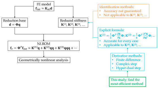
Figure 1.
Fundamental of non-intrusive NLROM and role of this study.
The rest of this paper is presented in the following order. Section 2 briefly presents the formula for computing the nonlinear stiffness matrix of a full-order model and the reduced stiffness of a reduced-order model. The first- to fourth-order derivatives of the nonlinear stiffness matrix with respect to the modal coordinates are then developed. Section 3 presents the formulas for calculating the derivatives of the nonlinear stiffness matrix by finite difference, complex step, and hyper-dual step methods. Section 4 presents a numerical example. The derivatives of the nonlinear stiffness matrix and the reduced stiffness obtained from numerical methods are compared with those obtained from the analytical method. The computation cost of the numerical methods is also discussed. Finally, conclusions and further work are drawn in Section 5.
2. Analytical Formulation
This Section presents analytical formulas for the derivatives of the nonlinear stiffness matrix of two-dimensional corotational beams with respect to the modal coordinates. First, the nonlinear stiffness matrix and the reduced stiffness are briefly presented in Section 2.1 and Section 2.2, respectively. Section 2.3 then develops the analytical formula for the derivatives of the nonlinear stiffness matrix with respect to the modal coordinates.
2.1. Nonlinear Stiffness Matrix
The corotational formula is used to describe the kinetics of beam elements in this study. The rigid motion and pure deformation of beam elements are separated using global and local coordinate systems. The global coordinate axes are fixed, while the local coordinate axes translate and rotate with the element. Therefore, the rigid body motion is eliminated in the local coordinate system, and the deformation of the element is obtained from the local displacement.
A two-dimensional Euler-Bernoulli beam element consisting of two nodes is considered. The global (X-Y) and local (Xl-Yl) coordinate systems of the element at initial (undeformed) and current (deformed) configurations are shown in Figure 2. The initial global coordinates of the two nodes are (x1, y1) and (x2, y2). The nodal displacement vector of the element in global coordinates at the current configuration is defined as
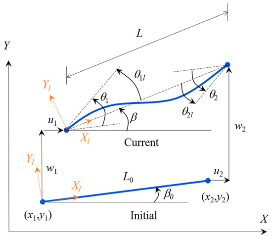
Figure 2.
Initial and current configuration of a beam element.
The local displacements of the element are given by
where ul, θ1l, and θ2l are the local axial displacement and local nodal rotations. L0 and L are the initial and current lengths of the element. β and β0 are counter clockwise rotations from the X-axis to Xl-axis at the initial and current configurations.
The local nodal internal forces of the element are given by
where N, M1, and M2 are axial force and end moments of the element. E, A, and I are Young’s modulus, cross-sectional area, and second moment of area of the element, respectively.
According to Yaw [29], the nonlinear stiffness matrix of the beam element at the current configuration is calculated as follows.
where
By substituting Equations (3) and (5)–(7) into Equation (4), ke can be written as
The components of ke are
The nonlinear stiffness matrix of the entire structure is constructed by assembling the nonlinear stiffness matrices of all the elements.
where Ae is the connectivity matrix of the eth element, and n is the number of elements.
2.2. Reduced Stiffness
The equation of motion for a full-order FE model is given by
where M denotes the mass matrix, C the damping matrix, fint the internal force vector, fext the external force vector, and d the nodal displacement vector. The cost of FE analysis is expensive, especially with large-sized models. In the model order reduction technique, linear mapping is used to reduce the number of unknown in the governing equation as follows.
where Φ is the reduction base, which includes vibration modes [4] or modal derivatives [30], or dual modes [31] or proper orthogonal modes [32]. In this study, mode shapes of free vibration around the initial configuration were considered. q is a set of modal coordinates, with r being much smaller than the number of degrees of freedom of the FE model. The dynamic equation of the reduced-order model becomes
If geometric nonlinearity is considered, the tangent stiffness matrix needs to be recalculated in each iteration. Computing the stiffness matrix using the FE code is expensive. To reduce the computation time, the tangential stiffness is approximated by a polynomial based on the Taylor series expansion as follows.
The first- and second-order derivatives of the nonlinear stiffness matrix with respect to the modal coordinates have the form of three- and four-dimensional arrays as follows.
The first- and second-order derivatives of the nonlinear stiffness matrix with respect to the modal coordinates have the form of five- and six-dimensional arrays, respectively. Computing the derivatives of the stiffness matrix with respect to modal coordinates is important because it affects the accuracy of the reduced-order model.
2.3. Analytical Derivative Formulation
Based on Equation (16), the first derivative of the nonlinear stiffness matrix with respect to the modal coordinate qm is given by
The connectivity matrices are constant, therefore
Similarly, the second, third and fourth derivatives of the nonlinear stiffness matrix are given by
Based on Equation (18), the derivatives of the elementary stiffness matrix with respect to modal coordinates can be expressed as follows
where φj, φm, φo, and φp are the mode shapes of mode j, m, o, and p, respectively. Since the nonlinear stiffness matrix of a beam element does not depend on the displacements of nodes not belonging to it, Equations (28)–(31) can be simplified as follows
where φe,j, φe,m, φe,o, and φe,p are the mode shapes of mode j, m, o, and p, respectively, for the eth element. Based on Equations (8)–(15), the derivatives of the elementary stiffness matrix with respect to the nodal displacement vector can be obtained using MATLAB/symbolic. By substituting Equations (32)–(35) into Equations (24)–(27), the derivatives of the nonlinear stiffness matrix with respect to the modal coordinates can be written as
3. Numerical Derivatives of Nonlinear Stiffness
This section presents the formulas for calculating the first- to fourth-order derivatives of the nonlinear stiffness matrix with respect to the modal coordinates by finite difference, complex step, and hyper-dual step methods.
3.1. Finite Difference Methods
When the variable x undergoes a small perturbation, the Taylor expansion of a function f can be expressed as:
The first derivative of the function can be derived directly from Equation (40a), which is known as the forward difference method.
where O(h) is the truncation error, proportional to h. Alternatively, the first derivative of the function can be derived from the difference of Equations (40a) and (40b), which is known as the central difference method.
The truncation error of the central difference is proportional to h2, which is much smaller than the truncation error of the forward difference. One can refer to [33] for more details on the finite difference methods.
The first- and second-order derivatives of the nonlinear stiffness matrix with respect to the modal coordinates at the initial configuration (d = 0) can be approximated using the forward difference method as follows.
where h is the step size. Algorithm 1 shows the algorithm for calculating the second-order derivative of nonlinear stiffness using the forward difference method. Figure 3 visualizes the selected points to calculate the first- and second-order derivatives.
| Algorithm 1 Algorithm to calculate the second-order derivative of nonlinear stiffness by forward difference method |
|
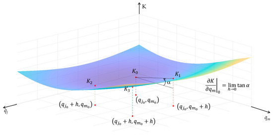
Figure 3.
Selected points to calculate the first- and second-order derivatives.
The third- and fourth-order derivatives of the nonlinear stiffness matrix are computed in the same manner as follows.
Detailed forward difference equations of the third- and fourth-order derivatives of the nonlinear stiffness matrix are given in Appendix A. To increase accuracy order of the derivatives, the central difference method can be used as follows.
Detailed central difference equations of the third- and fourth-order derivatives of the nonlinear stiffness matrix are given in Appendix A.
3.2. Complex Step Method
A simple formula for the complex step method to calculate the first-order derivative of a function has been proposed by Squire and Trapp [12]. It comes from the Taylor series expansion of a function with a complex variable as Equation (51). Taking the imaginary part of both sides of Equation (51), we get the first-order derivative of the function like Equation (52).
Therefore, the first-order derivative of the nonlinear stiffness matrix with respect to the modal coordinate qm at the initial configuration can be approximated using the complex step method as follows.
The formula for calculating the second-order derivative of a univariate function by the complex step method has been proposed in [13,14]. However, to the best of the authors’ knowledge, the complex step method has yet to be used to calculate the second partial derivative of a multivariable function. In this paper, we propose to combine the complex step method and the central difference method to calculate the second- to the fourth-order partial derivatives of the nonlinear stiffness matrix as follows.
Detailed complex step equations of the third- and fourth-order derivatives of the nonlinear stiffness matrix are given in Appendix A.
3.3. Hyper-Dual Step
The hyper-dual number has been proposed by Fike [18] to obtain the exact second-order derivative of functions. In this paper, we extend the hyper-dual number to calculate the fourth-order derivative of the nonlinear stiffness matrix. A hyper-dual number consisting of one real and fifteen unreal parts as follows is considered.
where
Taylor series expansion of a function with the hyper-dual number variable is
Due to the property of the hyper-dual number (Equation (58)), the Taylor series expansion stops precisely at the fourth-order derivative of the function. Therefore, the exact derivatives of the function can be obtained by taking the unreal parts of f(x) as follows.
The higher-order derivatives are suppressed resulting in the truncation error of the hyper-dual step method being zero. The hyper-dual number can be applied to compute the derivatives of the nonlinear stiffness matrix with respect to the modal coordinates as follows.
where
4. Results
A cantilever beam, as shown in Figure 4, is investigated in this Section. The beam’s length, width, and thickness are 1 m, 0.1 m, and 0.01 m, respectively. The density, Young’s modulus, and Poisson’s ratio are 7870 kg/m3, 205 GPa, and 0.28, respectively. The beam is discretized by forty elements. The first four vibration modes of the beam are shown in Figure 5. The accuracy of the derivatives of the beam nonlinear stiffness matrix, the accuracy of the reduced stiffness and the computation cost of the methods are evaluated in the following subsections.
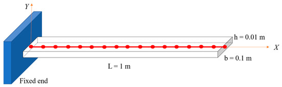
Figure 4.
Cantilever beam.
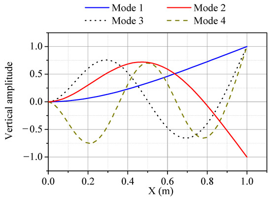
Figure 5.
The first four vibration modes of the beam.
4.1. Accuracy of Derivatives of Nonlinear Stiffness
The first-, second-, third- and fourth-order derivatives of the beam stiffness matrix with respect to the modal coordinates were computed by the forward difference, central difference, complex step, hyper-dual step, and analytical methods using MATLAB R2022a. The analytic derivatives are exact and are considered references. The derivatives obtained by numerical methods (the forward difference, central difference, complex step, and hyper-dual step methods) are compared with the references using relative error as follows.
where Dana and Dnum are the analytical and numerical derivatives of the nonlinear stiffness matrix, respectively. symbolizes the Frobenius norm.
Figure 6, Figure 7, Figure 8 and Figure 9 show the error and corresponding step size of the numerical derivatives of the nonlinear stiffness matrix with respect to the modal coordinates. The relative error on the derivatives obtained by the hyper-dual step method is constant, but that obtained by the forward difference, central difference, and complex step methods depends on the step size. Due to the truncation of Taylor series expansion, the derivatives obtained by the forward difference, central difference, and complex step methods have truncation errors, which are proportional to the step size. Therefore, the relative error on the derivatives obtained by these methods decreases when the step size decreases. However, when the step size is already too small, further reducing the step size causes the relative error to increase. The reason is that the subtractive cancellation error, which is derived from the finite precision of computers, increases as the step size decreases. The number of terms in the equations for the first-, second-, third- and fourth-order derivatives is rapidly increasing, leading to an increasingly significant role in the subtractive cancellation error. For the central difference method, the minimum value of the relative error and the corresponding step size increase from the first derivative (er = 10−13, h = 10−6) to the fourth derivative (er = 10−4, h = 10−2). Similar trends are also observed in the forward difference and the complex step methods.
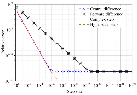
Figure 6.
The first derivative of the nonlinear stiffness matrix —errors of numerical methods.

Figure 7.
The second derivative of the nonlinear stiffness matrix —errors of numerical methods.
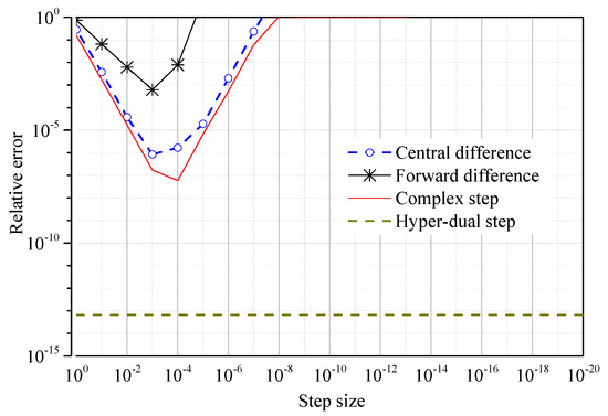
Figure 8.
The third derivative of the nonlinear stiffness matrix —errors of numerical methods.
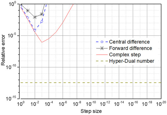
Figure 9.
The fourth derivative of the nonlinear stiffness matrix —errors of numerical methods.
Among the four numerical methods, the hyper-dual step method provides the most accurate derivatives of the nonlinear stiffness matrix with respect to the modal coordinates because they have neither the truncation error nor the subtractive cancellation error. The hyper-dual step method provides the first-order derivative with machine-level precision and the higher-order derivatives with slightly reduced precision. With an impressive level of precision in all four derivatives, the results from the hyper-dual step method can be considered exact. The results of the hyper-dual step method can be considered a reference when the analytical derivatives of the nonlinear stiffness have yet to be developed, such as the shell and solid FE models.
The forward difference, central difference, and complex step methods provide first-order derivatives with exceedingly minor errors but high-order derivatives with moderate errors. The forward difference method provides the derivatives with the lowest accuracy. Because the truncation error of the derivatives obtained by the forward difference method (O(h)) is more significant than that obtained by the central difference and complex step methods (O(h2)) when h is less than one. The complex step method can provide the first and second derivatives with exceedingly small relative errors and the third and fourth derivatives with moderate relative errors. The central difference method can provide the first derivative with exceedingly small relative error and the second, third, and fourth derivatives with moderate relative error. It can be seen from Figure 9 that the accuracy of the fourth-order derivative of the nonlinear stiffness matrix calculated by these methods is relatively low. Therefore, it is necessary to evaluate the accuracy of the quaternary reduced stiffness calculated from the fourth-order derivative of the nonlinear stiffness matrix by these methods.
4.2. Accuracy of NLROM
In this subsection, we verify the results of the NLROMs by comparing them with the results from Abaqus software in two examples: a clamped-clamped beam and a cantilever beam (CB). The dimensions of the two beams are the same and have been described at the beginning of Section 4. The beams are discretized using forty B31 elements in Abaqus.
4.2.1. Clamped-Clamped Beam
The first example is a clamped-clamped beam subjected to a concentrated force in the middle of the span. The parameters of NLROMs are summarized in Table 1. The reduction base of the NLROMs are the first four vibration modes (VMs) and the corresponding ten modal derivatives (MDs).

Table 1.
Parameters for NLROMs in Section 4.2.1.
Figure 10 shows the nonlinear static displacements of the clamped-clamped beam predicted from Abaqus and from NLROMs. All NLROMs constructed using different derivative methods provide the same results and are similar to those from Abaqus. Thus, all numerical derivative methods can be used to build the stiffness coefficients K(2) and K(3) of NLROM in the case of the clamped-clamped beam. Higher-order NLROMs all provide the same results as the third-order NLROMs, so computing the higher-order stiffness coefficients is unnecessary for the clamped-clamped beam.
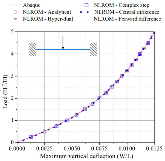
Figure 10.
Nonlinear static displacement of clamped-clamped beam.
4.2.2. Cantilever Beam
The second example is a cantilever beam subjected to a concentrated force at its free end. Figure 11 compares the static displacements of cantilever beams obtained from three NLROMs differing in order of nonlinear internal forces with the results obtained from Abaqus. All three NLROMs have the same reduction base including the first four vibration modes and the corresponding ten modal derivatives. The nonlinear stiffness coefficients of all three NLROMs are constructed using analytical derivative formulas. It can be seen that the third-order NLROM is only capable of accurately predicting the displacement of the cantilever beam when the normalized load is lower than 0.05. The inaccuracy of the standard third-order NLROM in predicting the displacements of cantilever structures was pointed out by Wang et al. [34]. They have proposed modifying the stiffness coefficients of the NLROM so that it could provide more accurate results. In this study, we propose increasing order of NLROM, and the results shown in Figure 11 demonstrate that the higher-order NLROM also predicts cantilever beam displacement more accurately.
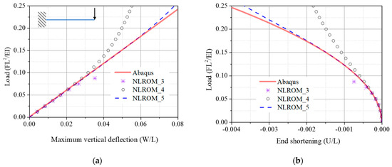
Figure 11.
Static displacement at the free end of the cantilever beam: (a) Vertical deflection; (b) End shortening. (NLROM_3: fin = K(1)q + K(2)qq + K(3)qqq; NLROM_4: fin = K(1)q + K(2)qq + K(3)qqq + K(4)qqqq; NLROM_5: fin = K(1)q + K(2)qq + K(3)qqq + K(4)qqqq + K(5)qqqqq).
Figure 12 illustrates the influence of the derivative method on the results of the fifth-order NLROM applied to the cantilever beam. The NLROMs constructed using the central difference, complex step and hyper-dual step methods exhibit the same accuracy as the NLROM using the analytic derivative formulas. Conversely, the forward difference method yields the lowest accuracy. Therefore, the central difference method is proposed to construct the NLROM for cantilever beams.
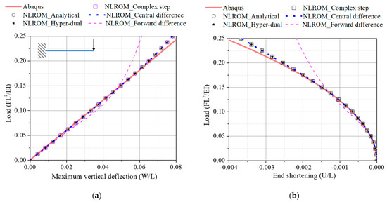
Figure 12.
Static displacements at the free end of cantilever beams obtained from Abaqus and fifth-order NLROMs: (a) Vertical deflection; (b) End shortening.
4.3. Computation Cost
Computation times of the four numerical methods are normalized and shown in Figure 13. Each derivative calculation was repeated ten times to find the average computation time. The average computation times are then normalized by dividing by the average computation time to determine using the forward difference method. All calculations are performed using MATLAB R2022a and a computer with Intel Core i7-8700K (3.70 GHz) processor and 16 GB RAM. The higher order of the derivative, the more computation time is required. The forward difference method requires the least computation time. The computation times of the central difference, complex step, and hyper-dual step methods are about 1.5, 3.5, and 7.5 times higher than that of the forward difference method.
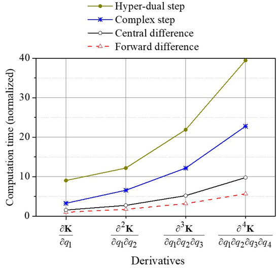
Figure 13.
Computation cost of numerical methods.
Based on the results presented in Figure 13, it is evident that the complex step and hyper-dual step methods for computing the derivatives of the nonlinear stiffness matrix are very expensive. This is especially true when computing the derivatives of the nonlinear stiffness matrix of shell and solid structures. As a result, for the purpose of NLROM construction, the central difference method is a suitable choice for computing the derivatives of the nonlinear stiffness matrix. This method provides a good balance between accuracy and computational cost.
5. Conclusions
In this study, we compared four numerical methods (forward difference, central difference, complex step and hyper-dual step) for calculating the derivatives of the nonlinear stiffness matrix to determine the nonlinear stiffness coefficient of NLROM. We proposed analytical formulas to compute the first-, second-, third- and fourth-order derivatives of the nonlinear stiffness matrix of the two-dimensional beam with respect to the modal coordinates. The analytical derivatives were considered the references to evaluate the accuracy of the numerical methods. The numerical methods were ranked in order of increasing accuracy: forward difference, central difference, complex step, and hyper-dual step. However, the computational cost also increases gradually from the forward difference method to the hyper-dual step method. The computational cost of the hyper-dual step method will be extremely expensive compared to the forward difference method when applied to shell or solid models. Other advantages of the forward and central difference methods over the complex and hyper-dual step methods are ease of implementation and compatibility with commercial FE software. For clamped-clamped beams, the third-order NLROM built by any numerical derivative method has good accuracy. In the case of cantilever beams, a fifth-order NLROM is necessary, and the nonlinear stiffness coefficients of the NLROM can be constructed using any of the derivative methods except for the forward difference method. From the above evaluation, the central difference method is the most effective method for computing the derivative of the nonlinear stiffness matrix to determine the nonlinear stiffness coefficients for the NLROM of beam structures. However, it is essential to note that the step size plays a significant role in the accuracy of the forward and central difference methods, as well as the complex step method. Therefore, an optimal step size needs to be investigated before constructing the NLROM.
In the future, we plan to develop the NLROM for nonlinear vibration prediction of plate structures. Additionally, improving the hyper-dual step method in terms of computational cost is also a promising direction for future research.
Author Contributions
Conceptualization, T.A.B. and J.-S.K.; methodology, T.A.B. and J.-S.K.; formal analysis, T.A.B. and J.-S.K.; investigation, T.A.B., J.-S.K. and J.P.; resources, J.P.; data curation, T.A.B.; writing—original draft preparation, T.A.B., J.-S.K. and J.P.; writing—review and editing, T.A.B., J.-S.K. and J.P.; visualization, T.A.B., J.-S.K. and J.P.; supervision, J.-S.K. and J.P.; project administration, J.P.; funding acquisition, J.P. All authors have read and agreed to the published version of the manuscript.
Funding
This research was funded by the National Research Foundation of Korea (NRF), grant number [NRF-2018R1A2B 2004207], and the MSIT (Ministry of Science and ICT), Korea, under the Grand Information Technology Research Center support program, grant number (IITP-2022-2020-0-01612).
Data Availability Statement
Not applicable.
Acknowledgments
The authors gratefully acknowledge the funding provided by the National Research Foundation of Korea (NRF) [NRF-2018R1A2B 2004207] and the MSIT (Ministry of Science and ICT), Korea, under the Grand Information Technology Research Center support program (IITP-2022-2020-0-01612) supervised by the IITP (Institute for Information & communications Technology Planning & Evaluation).
Conflicts of Interest
The authors declare no conflict of interest.
Appendix A
The third- and fourth-order derivatives of the tangent stiffness matrix with respect to the modal coordinates can be approximated using the forward difference method as follows.
The third- and fourth-order derivatives of the nonlinear stiffness matrix can be approximated using the central difference method as follows.
The third- and fourth-order derivatives of the nonlinear stiffness matrix can be approximated using the complex step method as follows.
References
- Touzé, C.; Vizzaccaro, A.; Thomas, O. Model order reduction methods for geometrically nonlinear structures: A review of nonlinear techniques. Nonlinear Dyn. 2021, 105, 1141–1190. [Google Scholar] [CrossRef]
- Mignolet, M.P.; Przekop, A.; Rizzi, S.A.; Spottswood, S.M. A review of indirect/non-intrusive reduced order modeling of nonlinear geometric structures. J. Sound Vib. 2013, 332, 2437–2460. [Google Scholar] [CrossRef]
- Rutzmoser, J. Model Order Reduction for Nonlinear Structural Dynamics. Ph.D. Thesis, Technical University of Munich, Munich, Germany, 2018. [Google Scholar]
- Muravyov, A.A.; Rizzi, S.A. Determination of nonlinear stiffness with application to random vibration of geometrically nonlinear structures. Comput. Struct. 2003, 81, 1513–1523. [Google Scholar] [CrossRef]
- Perez, R.; Wang, X.Q.; Mignolet, M.P. Nonintrusive structural dynamic reduced order modeling for large deformations: Enhancements for complex structures. J. Comput. Nonlinear Dyn. 2014, 9, 031008. [Google Scholar] [CrossRef]
- Cai, M.; Li, C. Numerical approaches to fractional integrals and derivatives: A review. Mathematics 2020, 8, 43. [Google Scholar] [CrossRef]
- Treanţă, S. Recent advances of constrained variational problems involving second-order partial derivatives: A review. Mathematics 2022, 10, 2599. [Google Scholar] [CrossRef]
- Kirsch, U.; Bogomolni, M.; Keulen, F.V. Efficient finite difference design sensitivities. AIAA J. 2005, 43, 399–405. [Google Scholar] [CrossRef]
- Xu, S.; Liu, J.; Ma, Y. Residual stress constrained self-support topology optimization for metal additive manufacturing. Comput. Methods Appl. Mech. Eng. 2022, 389, 114380. [Google Scholar] [CrossRef]
- Lyness, J.N.; Moler, C.B. Numerical differentiation of analytic functions. SIAM J. Numer. Anal. 1967, 4, 202–210. [Google Scholar] [CrossRef]
- Lyness, J.N. Numerical algorithms based on the theory of complex variables. In Proceedings of the 22nd ACM National Conference, Washington, DC, USA, 1 January 1967. [Google Scholar] [CrossRef]
- Squire, W.; Trapp, G. Using complex variables to estimate derivatives of real functions. SIAM Rev. 1998, 10, 100–112. [Google Scholar] [CrossRef]
- Lai, K.L.; Crassidis, J.L. Extensions of the first and second complex-step derivative approximations. J. Comput. Appl. Math. 2008, 219, 276–293. [Google Scholar] [CrossRef]
- Abreu, R.; Stich, D.; Morales, J. On the generalization of the Complex Step Method. J. Comput. Appl. Math. 2013, 241, 84–102. [Google Scholar] [CrossRef]
- Pérez-Foguet, A.; Rodríguez-Ferran, A.; Huerta, A. Numerical differentiation for local and global tangent operators in computational plasticity. Comput. Meth. Appl. Mech. Eng. 2000, 189, 277–296. [Google Scholar] [CrossRef]
- Kim, S.; Ryu, J.; Cho, M. Numerically generated tangent stiffness matrices using the complex variable derivative method for nonlinear structural analysis. Comput. Meth. Appl. Mech. Eng. 2011, 200, 403–413. [Google Scholar] [CrossRef]
- Tanaka, M.; Fujikawa, M.; Balzani, D.; Schröder, J. Robust numerical calculation of tangent moduli at finite strains based on complex-step derivative approximation and its application to localization analysis. Comput. Meth. Appl. Mech. Eng. 2014, 269, 454–470. [Google Scholar] [CrossRef]
- Fike, J.A. Multi-Objective Optimization Using Hyper-Dual Numbers. Ph.D. Thesis, Stanford University, Stanford, CA, USA, 2013. [Google Scholar]
- Tanaka, M.; Sasagawa, T.; Omote, R.; Fujikawa, M.; Balzani, D.; Schröder, J. A highly accurate 1st- and 2nd-order differentiation scheme for hyperelastic material models based on hyper-dual numbers. Comput. Meth. Appl. Mech. Eng. 2015, 283, 22–45. [Google Scholar] [CrossRef]
- Kiran, R.; Khandelwal, K. Automatic implementation of finite strain anisotropic hyperelastic models using hyper-dual numbers. Comput. Mech. 2015, 55, 229–248. [Google Scholar] [CrossRef]
- Lantoine, G.; Russell, R.P.; Dargent, T. Using multicomplex variables for automatic computation of high-order derivatives. ACM Trans. Math. Softw. 2012, 38, 1–21. [Google Scholar] [CrossRef]
- Aristizabal, M.; Ramirez-Tamayo, D.; Garcia, M.; Aguirre-Mesa, A.; Montoya, A.; Millwater, H. Quaternion and octonion-based finite element analysis methods for computing multiple first order derivatives. J. Comput. Phys. 2019, 397, 108831. [Google Scholar] [CrossRef]
- Rutzmoser, J.B.; Rixen, D.J.; Tiso, P.; Jain, S. Generalization of quadratic manifolds for reduced order modeling of nonlinear structural dynamics. Comput. Struct. 2017, 192, 196–209. [Google Scholar] [CrossRef]
- Vizzaccaro, A.; Salles, L.; Touzé, C. Comparison of nonlinear mappings for reduced-order modelling of vibrating structures: Normal form theory and quadratic manifold method with modal derivatives. Nonlinear Dyn. 2021, 103, 3335–3370. [Google Scholar] [CrossRef]
- Mahdiabadi, M.K.; Tiso, P.; Brandt, A.; Rixen, D.J. A non-intrusive model-order reduction of geometrically nonlinear structural dynamics using modal derivatives. Mech. Syst. Signal Process. 2021, 147, 107126. [Google Scholar] [CrossRef]
- Jeong, Y.M.; Kim, J.S. On the stable mode selection for efficient component mode synthesis of geometrically nonlinear beams. J. Mech. Sci. Technol. 2020, 34, 2961–2973. [Google Scholar] [CrossRef]
- Talebitooti, R.; Zarastvand, M.R. The effect of nature of porous material on diffuse field acoustic transmission of the sandwich aerospace composite doubly curved shell. Aerosp. Sci. Technol. 2018, 78, 157–170. [Google Scholar] [CrossRef]
- Seilsepour, H.; Zarastvand, M.; Talebitooti, R. Acoustic insulation characteristics of sandwich composite shell systems with double curvature: The effect of nature of viscoelastic core. J. Vib. Control 2023, 29, 1076–1090. [Google Scholar] [CrossRef]
- Yaw, L.L. 2D Corotational Beam Formulation; Walla Walla University: Washington, DC, USA, 2009. [Google Scholar]
- Sombroek, C.S.M.; Tiso, P.; Renson, L.; Kerschen, G. Numerical computation of nonlinear normal modes in a modal derivative subspace. Comput. Struct. 2018, 195, 34–46. [Google Scholar] [CrossRef]
- Kim, K.; Radu, A.G.; Wang, X.Q.; Mignolet, M.P. Nonlinear reduced order modeling of isotropic and functionally graded plates. Int. J. Non-Linear Mech. 2013, 49, 100–110. [Google Scholar] [CrossRef]
- Rizzi, S.A.; Przekop, A. System identification-guided basis selection for reduced-order nonlinear response analysis. J. Sound Vib. 2008, 315, 467–485. [Google Scholar] [CrossRef]
- Olver, P.J. Finite Differences. In Introduction to Partial Differential Equations, 2nd ed.; Sheldon, A., Kenneth, R., Eds.; Springer: Cham, Switzerland, 2020; pp. 181–214. [Google Scholar] [CrossRef]
- Wang, X.Q.; Khanna, V.; Kim, K.; Mignolet, M.P. Nonlinear Reduced-Order Modeling of Flat Cantilevered Structures: Identification Challenges and Remedies. J. Aerosp. Eng. 2021, 34, 04021085. [Google Scholar] [CrossRef]
Disclaimer/Publisher’s Note: The statements, opinions and data contained in all publications are solely those of the individual author(s) and contributor(s) and not of MDPI and/or the editor(s). MDPI and/or the editor(s) disclaim responsibility for any injury to people or property resulting from any ideas, methods, instructions or products referred to in the content. |
© 2023 by the authors. Licensee MDPI, Basel, Switzerland. This article is an open access article distributed under the terms and conditions of the Creative Commons Attribution (CC BY) license (https://creativecommons.org/licenses/by/4.0/).