A New Approach for Solving Nonlinear Fractional Ordinary Differential Equations

Abstract

Recently, researchers have been interested in studying fractional differential equations and their solutions due to the wide range of their applications in many scientific fields. In this paper, a new approach called the Hussein–Jassim (HJ) method is presented for solving nonlinear fractional ordinary differential equations. The new method is based on a power series of fractional order. The proposed approach is employed to obtain an approximate solution for the fractional differential equations. The results of this study show that the solutions obtained from solving the fractional differential equations are highly consistent with those obtained by exact solutions.

1. Introduction

Engineering-related problems, applied mathematics, and physics are significantly impacted by nonlinear phenomena. Many of these physical phenomena are represented by nonlinear differential equations. In both physics and mathematics, differential equations remain an important issue requiring innovative approaches to find precise or approximate solutions. Since the majority of brand-new linear and nonlinear equations lack an exact analytic solution, numerical techniques have mostly been employed to solve them [1].

During the past decades, fractional differential equations (FDEs) have appeared more and more frequently in different research areas, and they can offer an improved description of many vital phenomena in electromagnetics, acoustics, viscoelasticity, electrochemistry, cosmology, and materials science. Consequently, considerable attention has been given to the solution of the fractional differential equations [2].

The exploration and development of numerical techniques particularly designed to solve fractional differential equations have been inspired by the growing interest in applications of fractional calculus. It is more difficult to find analytical solutions for FDEs than it is to solve conventional ordinary differential equations (ODEs), and most of the time, the answer can only be approximated numerically [3].

Mathematical models called nonlinear differential equations (NDEs) are used to explain complicated events that appear in our environment. Numerous applications of science and engineering, including those involving fluid dynamics, plasma physics, hydrodynamics, solid state physics, optical fibers, acoustics, and other fields, use nonlinear equations. Recently, numerous researchers have focused their on NDEs solutions utilizing a variety of techniques, including the Adomian decomposition method [4], the variational iteration method [5], the homotopy perturbation method [6], the homotopy analysis method [7], the differential transform method [8], the F-expansion method [9], the Exp-function method [10], the sine–cosine method [11], the reduced differential transform method [12], the Sumudu homotopy perturbation method [13], the Sumudu Adomian decomposition method [14], the Daftardar–Jafari method [15], and others [16,17,18,19,20,21,22,23,24,25,26,27,28,29,30,31,32,33,34,35,36,37,38,39].

In this paper, a new iterative method for solving fractional ordinary differential equations (FODEs) is presented and discussed. This method is mainly based on fractional power series. In order to introduce the method, we must mention several concepts and definitions.

 Definition 1

([40,41,42]). If $f\left(x\right)\in C\left(\right[a,b\left]\right)$,$\alpha >0$, and $a<x<b$, then the Riemann–Liouville fractional integral of order$\alpha$ is given by as

$$I_x^{\alpha }f\left(x\right)=\frac{1}{\mathsf{\Gamma }\left(\alpha \right)}{\int }_a^x \frac{f\left(t\right)}{(x-t{)}^{1-\alpha }}dt,$$

where $\Gamma$ is the well-known Gamma function.

The properties of the Riemann–Liouville fractional integral are as follows:

• $I_x^{\alpha }{I}_x^{\sigma }f\left(x\right)=I_x^{\alpha +\sigma }f\left(x\right)$;
• $I_x^{\alpha }{I}_x^{\sigma }f\left(x\right)=I_x^{\sigma }{I}_x^{\alpha }f\left(x\right)$;
• $I_x^{\alpha }{x}^{\beta }=\frac{\Gamma (\beta +1)}{\Gamma (\alpha +\beta +1)}{x}^{\alpha +\beta }$;

where $\mathsf{\alpha }$ and $\mathsf{\sigma }$ are greater than zero and $\mathsf{\beta }$ is a real number.

 Definition 2

([41,42]). The fractional derivative of $f(x)$ in the Caputo sense is defined as

$${}_a{}^C{D}_x^{\alpha }f(x)=\frac{1}{\mathsf{\Gamma }(m-\alpha )}{\int }_a^x (x-\tau {)}^{m-\alpha -1}{f}^{(m)}(\tau )d\tau ,$$

where $m-1<\alpha \le m,m\in \mathbb{N}$.

The following are the basic properties of the operator ${}_a{}^C{D}_x^{\alpha }$:

 1. 

${}_a{}^C{D}_x^{\alpha }\lambda =0;$

 2. 

${}_a{}^C{D}_x^{\alpha }{I}^{\alpha }f\left(x\right)=f(x)$;

 3. 

${}_a{}^C{D}_x^{\alpha }{x}^{\beta }=\frac{\Gamma (\beta +1)}{\Gamma (\beta -\alpha +1)}{x}^{\beta -\alpha }$;

 4. 

${}_a{}^C{D}_x^{\alpha }{}_a{}^C{D}_x^{\sigma }f\left(x\right)={}_a{}^C{D}_x^{\alpha +\sigma }f\left(x\right)={}_a{}^C{D}_x^{\sigma }{}_a{}^C{D}_x^{\alpha }f(x)$;

 5. 

${}_a{}^C{D}_x^{\alpha }(\lambda f(x)+\delta g(x))=\lambda {}_a{}^C{D}_x^{\alpha }f(x)+\delta {}_a{}^C{D}_x^{\sigma }g(x)$;

 6. 

$I^{\alpha }{}_a{}^C{D}_x^{\alpha }f(x)=f(x)-{\sum }_{k=0}^{m-1} f^{(k)}(0)\frac{t^k}{k!}$;

where $\mathsf{\lambda }$ and $\mathsf{\delta }$ are constants.

 Definition 3

([42]). The Mittag–Leffler function $E_{\alpha }\left(x\right)$ is defined as

$$E_{\alpha }\left(x\right)={\sum }_{m=0}^{\mathrm{\infty }} \frac{x^m}{\mathsf{\Gamma }\left(m\alpha +1\right)}.$$

For special values $\mathsf{\alpha }$, the Mittag–Leffer function is given by the following:

• $E_0(x)=\frac{1}{1-x}$;
• $E_1\left(x\right)=e^x$;
• $E_2\left(x^2\right)=\cosh \left(x\right)$;
• $E_2\left(-x^2\right)=cos\left(x\right).$

2. Analysis of the New Method

Consider the following initial value problem in the FODE sense

$${}^{C}D_t^{\sigma }𝓎\left(t\right)+\mathcal{N}\left(𝓎\left(t\right)\right)=g\left(t^{\sigma }\right), 0<\sigma \le 1$$

(1)

with initial condition $𝓎\left(0\right)=\lambda$, where $𝓎$ is an analytical function, ${}^{C}D_t^{\sigma }$ is the Caputo operator, $\mathcal{N}$ is a nonlinear operator, and $g\left(t^{\sigma }\right)$ is a known function.

By taking the Riemann–Liouville operator of fractional integration to both side of Equation (1), we obtain

$$𝓎\left(t\right)=\lambda +I_t^{\sigma }\left(g\left(t^{\sigma }\right)-\mathcal{N}\left(𝓎\left(t\right)\right)\right).$$

(2)

Now, we rewrite the right side of Equation (2) as an infinite fractional power series:

$$\lambda +I_t^{\sigma }\left(g\left(t^{\sigma }\right)-\mathcal{N}\left(𝓎\left(t\right)\right)\right)=a_0+a_1{t}^{\sigma }+a_2{t}^{2\sigma }+\cdots ={\sum }_{i=0}^{\infty }{a}_i{t}^{i\sigma },$$

(3)

where $a_0,a_1,\dots$ are coefficients.

By taking the fractional derivative of Caputo ${}^{C}D_t^{i\sigma }$ where $i=\mathrm{0,1},2,\dots$, for both sides of Equation (3) at $t=0,$ we obtain

$$\left\{\begin{array}{c}{a}_0=𝓎\left(0\right)=\lambda ,\\ a_1=\frac{{\left(g\left(t^{\sigma }\right)-\mathcal{N}\left(𝓎\left(t\right)\right)\right)}_{t=0}}{\mathsf{\Gamma }\left(\sigma +1\right)},\\ a_2=\frac{{}^{C}D_t^{\sigma }{\left(g\left(t^{\sigma }\right)-\mathcal{N}\left(𝓎\left(t\right)\right)\right)}_{t=0}}{\mathsf{\Gamma }\left(2\sigma +1\right)},\\ a_3=\frac{{}^{C}D_t^{2\sigma }{\left(g\left(t^{\sigma }\right)-\mathcal{N}\left(𝓎\left(t\right)\right)\right)}_{t=0}}{\mathsf{\Gamma }\left(3\sigma +1\right)},\\ ⋮\end{array}\right.$$

(4)

Substituting Equation (4) into Equation (3) results in

$$𝓎\left(t\right)={\sum }_{i=0}^{\infty }\frac{{{}^{C}D_t^{(i-1)\sigma }\left(g\left(t^{\sigma }\right)-\mathcal{N}\left(𝓎\left(t\right)\right)\right)}_{t=0}}{\mathsf{\Gamma }(i\sigma +1)}{t}^{i\sigma }.$$

(5)

Now, suppose that $𝓎\left(t\right)$ is a solution of Equation (5), which can be expressed as

$$𝓎\left(t\right)={\sum }_{i=0}^{\infty }{𝓎}_i$$

(6)

Substituting Equation (6) into Equation (5) yields

$${\sum }_{i=0}^{\infty }{𝓎}_i={\sum }_{i=0}^{\infty }\frac{{{}^{C}D_t^{(i-1)\sigma }\left(g\left(t^{\sigma }\right)-\mathcal{N}\left(\sum _{i=0}^{\infty }{𝓎}_i\right)\right)}_{t=0}}{\mathsf{\Gamma }(i\sigma +1)}{t}^{i\sigma }.$$

(7)

By setting $i=i+1$ in the left side of Equation (7), we obtain

$${𝓎}_0+{\sum }_{i=0}^{\infty }{𝓎}_{i+1}=\lambda +{\sum }_{i=1}^{\infty }\frac{{{}^{C}D_t^{(i-1)\sigma }\left(g\left(t^{\sigma }\right)-\mathcal{N}\left(\sum _{i=0}^{\infty }{𝓎}_i\right)\right)}_{t=0}}{\mathsf{\Gamma }(i\sigma +1)}{t}^{i\sigma }.$$

(8)

We compare the two sides of Equation (8):

$$\left\{\begin{array}{c}{𝓎}_0=𝓎\left(0\right)=\lambda ,\\ {𝓎}_1=\frac{{\left(g\left(t^{\sigma }\right)-\mathcal{N}\left({𝓎}_0\right)\right)}_{t=0}}{\mathsf{\Gamma }(\sigma +1)}{t}^{\sigma },\\ {𝓎}_2=\frac{{}^{C}D_t^{\sigma }{\left(g\left(t^{\sigma }\right)-\mathcal{N}\left({𝓎}_0+{𝓎}_1\right)\right)}_{t=0}}{\mathsf{\Gamma }(2\sigma +1)}{t}^{2\sigma },\\ {𝓎}_3=\frac{{}^{C}D_t^{2\sigma }{\left(g\left(t^{\sigma }\right)-\mathcal{N}\left({𝓎}_0+{𝓎}_1+{𝓎}_2\right)\right)}_{t=0}}{\mathsf{\Gamma }(3\sigma +1)}{t}^{3\sigma },\\ ⋮\\ {𝓎}_{i+1}=\frac{{}^{C}D_t^{i\sigma }{\left(g\left(t^{\sigma }\right)-\mathcal{N}\left(\sum _{j=0}^i{𝓎}_j\right)\right)}_{t=0}}{\mathsf{\Gamma }\left(\right(i+1)\sigma +1)}{t}^{(i+1)\sigma }.\end{array}\right.$$

(9)

Therefore, the approximate solution can be formulated as follows:

$$𝓎\left(t\right)={𝓎}_0+{𝓎}_1+{𝓎}_3+\cdots ={\sum }_{i=0}^{\infty }{𝓎}_i.$$

3. Convergence of the New Method

 Theorem 1. 

The proposed method used to solve Equation (1) is equivalent to determine the following sequence:

$$\begin{gathered} {\mathcal{S}}_{\eta }={𝓎}_1+{𝓎}_2+{𝓎}_3+\cdots +{𝓎}_{\eta }, \\ {\mathcal{S}}_0=0 \end{gathered}$$

(10)

By using the iterative scheme:

$${\mathcal{S}}_{\eta +1}={\sum }_{i=1}^{\eta +1}\frac{{}^{C}D_t^{(i-1)\sigma }{\left(g\left(t^{\sigma }\right)-\mathcal{N}\left(\sum _{j=0}^{i-1}{𝓎}_j\right)\right)}_{t=0}}{\mathsf{\Gamma }(i\sigma +1)}{t}^{i\sigma }.$$

(11)

 Proof. 

For $\eta =0$, Equation (11) can be written as

$${\mathcal{S}}_1=\frac{{\left(g\left(t^{\sigma }\right)-\mathcal{N}\left({𝓎}_0\right)\right)}_{t=0}}{\mathsf{\Gamma }(\sigma +1)}{t}^{\sigma },$$

then,

$${𝓎}_1=\frac{{\left(g\left(t^{\sigma }\right)-\mathcal{N}\left({𝓎}_0\right)\right)}_{t=0}}{\mathsf{\Gamma }(\sigma +1)}{t}^{\sigma }.$$

For $\eta =1$, Equation (11) can be expressed as

$$\begin{array}{ll}{\mathcal{S}}_2& =\sum _{i=1}^2\frac{{}^{C}D_t^{(i-1)\sigma }{\left(g\left(t^{\sigma }\right)-\mathcal{N}\left(\sum _{j=0}^{i-1}{𝓎}_j\right)\right)}_{t=0}}{\mathsf{\Gamma }(i\sigma +1)}{t}^{i\sigma },\\ & =\frac{{\left(g\left(t^{\sigma }\right)-\mathcal{N}\left({𝓎}_0\right)\right)}_{t=0}}{\mathsf{\Gamma }(\sigma +1)}{t}^{\sigma }+\frac{{}^{C}D_t^{\sigma }{\left(g\left(t^{\sigma }\right)-\mathcal{N}\left({𝓎}_0+{𝓎}_1\right)\right)}_{t=0}}{\mathsf{\Gamma }(2\sigma +1)}{t}^{2\sigma },\\ & ={𝓎}_1+\frac{{}^{C}D_t^{\sigma }{\left(g\left(t^{\sigma }\right)-\mathcal{N}\left({𝓎}_0+{𝓎}_1\right)\right)}_{t=0}}{\mathsf{\Gamma }(2\sigma +1)}{t}^{2\sigma }\end{array}$$

According to ${\mathcal{S}}_2={𝓎}_1+{𝓎}_2$, the latter equation can be written as

$${𝓎}_2=\frac{{}^{C}D_t^{\sigma }{\left(g\left(t^{\sigma }\right)-\mathcal{N}\left({𝓎}_0+{𝓎}_1\right)\right)}_{t=0}}{\mathsf{\Gamma }(2\sigma +1)}{t}^{2\sigma }.$$

This theorem will be proved by strong induction. Let us assume that

$${𝓎}_{m+1}=\frac{{}^{C}D_t^{m\sigma }{\left(g\left(t^{\sigma }\right)-\mathcal{N}\left(\sum _{j=0}^m{𝓎}_j\right)\right)}_{t=0}}{\mathsf{\Gamma }\left(\right(m+1)\sigma +1)}{t}^{(m+1)\sigma },$$

where $m=\mathrm{1,2},3,\dots ,\eta -1$, so

$$\begin{array}{ll}{\mathcal{S}}_{\eta +1}& =\sum _{i=1}^{\eta +1}\frac{{}^{C}D_t^{(i-1)\sigma }{\left(g\left(t^{\sigma }\right)-\mathcal{N}\left(\sum _{j=0}^{i-1}{𝓎}_j\right)\right)}_{t=0}}{\mathsf{\Gamma }(i\sigma +1)}{t}^{i\sigma },\\ & =\frac{{\left(g\left(t^{\sigma }\right)-\mathcal{N}\left({𝓎}_0\right)\right)}_{t=0}}{\mathsf{\Gamma }(\sigma +1)}{t}^{\sigma }+\cdots +\frac{{}^{C}D_t^{\eta \sigma }{\left(g\left(t^{\sigma }\right)-\mathcal{N}\left(\sum _{j=0}^{\eta }{𝓎}_j\right)\right)}_{t=0}}{\mathsf{\Gamma }\left(\left(\eta +1\right)\sigma +1\right)}{t}^{\left(\eta +1\right)\sigma },\\ & ={𝓎}_1+{𝓎}_2+\cdots +{𝓎}_{\eta }+\frac{{}^{C}D_t^{\eta \sigma }{\left(g\left(t^{\sigma }\right)-\mathcal{N}\left(\sum _{j=0}^{\eta }{𝓎}_j\right)\right)}_{t=0}}{\mathsf{\Gamma }\left(\left(\eta +1\right)\sigma +1\right)}{t}^{\left(\eta +1\right)\sigma }.\end{array}$$

Using Equation (10), the following equation can be obtained:

$${𝓎}_{\eta +1}=\frac{{}^{C}D_t^{\eta \sigma }{\left(g\left(t^{\sigma }\right)-\mathcal{N}\left(\sum _{j=0}^{\eta }{𝓎}_j\right)\right)}_{t=0}}{\mathsf{\Gamma }\left(\left(\eta +1\right)\sigma +1\right)}{t}^{\left(\eta +1\right)\sigma }.$$

Hence, the theorem is proved, as the latter equation is similar to Equation (9). □

 Theorem 2. 

Let $\mathcal{B}$ be a Banach space.

 I. 

$\sum _{i=0}^{\mathrm{\infty }}{𝓎}_i$ obtained by Equation (9) convergence to $\mathcal{S}\in \mathcal{B}$, if

$$\exists \left(0\le \mathcal{E}<1\right),such that\left(\forall \eta \in \mathbb{N}\Rightarrow ‖{𝓎}_{\eta }‖\le \mathcal{E}‖{𝓎}_{\eta -1}‖\right).$$

(12)

 II. 

$\mathcal{S}=\sum _{\eta =1}^{\mathrm{\infty }}{𝓎}_{\eta },$ satisfies in

$$\mathcal{S}=\sum _{i=1}^{\infty }\frac{{}^{C}D_t^{(i-1)\sigma }{\left(g\left(t^{\sigma }\right)-\mathcal{N}\left(\sum _{i=0}^{\infty }{𝓎}_i\right)\right)}_{t=0}}{\mathsf{\Gamma }(i\sigma +1)}{t}^{i\sigma }.$$

(13)

 Proof. 

• We must prove that ${\left\{\mathcal{S}\right\}}_{\eta =0}^{\infty }$ is a Cauchy sequence in the Banach space $\mathcal{B}$.

From Equation (12), we have

$$\begin{array}{l}‖{\mathcal{S}}_{\eta +1}-{\mathcal{S}}_{\eta }‖=‖\sum _{i=0}^{\eta +1}{𝓎}_i-\sum _{i=0}^{\eta }{𝓎}_i‖=‖{𝓎}_{\eta +1}‖,\\ \le \mathcal{E}\left||{𝓎}_{\eta }|\right|\le {\mathcal{E}}^2\left||{𝓎}_{\eta -1}|\right|\le {\mathcal{E}}^3\left||{𝓎}_{\eta -2}|\right|\le \cdots \le {\mathcal{E}}^{\eta +1}\left|\left|{𝓎}_0\right|\right|.\end{array}$$

(14)

For all $\eta ,m\in \mathbb{N},\eta \ge m,$

$$\begin{array}{ll}‖{\mathcal{S}}_{\eta }-{\mathcal{S}}_m‖& =‖\left({\mathcal{S}}_{\eta }-{\mathcal{S}}_{\eta -1}\right)+\left({\mathcal{S}}_{\eta -1}-{\mathcal{S}}_{\eta -2}\right)+\cdots +\left({\mathcal{S}}_{m+1}-{\mathcal{S}}_m\right)‖,\\ & \le ‖{\mathcal{S}}_{\eta }-{\mathcal{S}}_{\eta -1}‖+‖{\mathcal{S}}_{\eta -1}-{\mathcal{S}}_{\eta -2}‖+\cdots +‖{\mathcal{S}}_{m+1}-{\mathcal{S}}_m‖,\\ & \le {\mathcal{E}}^{\eta }‖{𝓎}_0‖\le {\mathcal{E}}^{\eta -1}‖{𝓎}_0‖\le {\mathcal{E}}^{\eta -2}‖{𝓎}_0‖\le \cdots \le {\mathcal{E}}^{m+1}‖{𝓎}_0‖,\\ & \le {\mathcal{E}}^{m+1}\left|\left|{𝓎}_0\right|\right|\left({\mathcal{E}}^{\eta -m-1}+{\mathcal{E}}^{\eta -m-2}+\cdots +1\right),\\ & =\frac{1-{\mathcal{E}}^{\eta -m}}{1-\mathcal{E}}{\mathcal{E}}^{m+1}‖{𝓎}_0‖.\end{array}$$

(15)

Since $\left({\mathcal{E}}^{\eta -m-1}+\cdots +1\right)$ is a geometric series and $0\le \mathcal{E}<1$, then $\underset{\eta ,m\to \mathrm{\infty }}{\lim }‖{\mathcal{S}}_{\eta }-{\mathcal{S}}_m‖=0.$

Thus, $\left\{{\mathcal{S}}_{\eta }\right\}$ is a Cauchy sequence in the Banach space, and it is convergent. In other words $\exists \mathcal{S}\in \mathcal{B}$, such that ${\mathrm{l}\mathrm{i}\mathrm{m}}_{\eta \to \mathrm{\infty }} {\mathcal{S}}_{\eta }={\sum }_{\eta =1}^{\mathrm{\infty }} {𝓎}_{\eta }=\mathcal{S}$.

II.

Equation (11) can be written as

$$\begin{array}{ll}\underset{\eta \to \infty }{\mathrm{l}\mathrm{i}\mathrm{m}}{\mathcal{S}}_{\eta +1}& =\underset{\eta \to \infty }{\lim }\sum _{i=1}^{\eta +1}\frac{{}^{C}D_t^{(i-1)\sigma }{\left(g\left(t^{\sigma }\right)-\mathcal{N}\left(\sum _{j=0}^{i-1}{𝓎}_j\right)\right)}_{t=0}}{\mathsf{\Gamma }(i\sigma +1)}{t}^{i\sigma },\\ & =\sum _{i=1}^{\infty }\frac{{}^{C}D_t^{(i-1)\sigma }{\left(g\left(t^{\sigma }\right)-\mathcal{N}\left(\sum _{j=0}^{i-1}{𝓎}_j\right)\right)}_{t=0}}{\mathsf{\Gamma }(i\sigma +1)}{t}^{i\sigma }.\end{array}$$

Since the upper bound of the sum approaches infinity, we obtain the following equation:

$$\mathcal{S}={\sum }_{i=1}^{\infty }\frac{{}^{C}D_t^{(i-1)\sigma }{\left(g\left(t^{\sigma }\right)-\mathcal{N}\left(\sum _{i=0}^{\infty }{𝓎}_i\right)\right)}_{t=0}}{\mathsf{\Gamma }(i\sigma +1)}{t}^{i\sigma }={\sum }_{i=1}^{\infty }{𝓎}_i.$$

□

 Theorem 3. 

The following equation (Equation (13))

$$\mathcal{S}={\sum }_{i=1}^{\infty }\frac{{}^{C}D_t^{(i-1)\sigma }{\left(g\left(t^{\sigma }\right)-\mathcal{N}\left(\sum _{i=0}^{\infty }{𝓎}_i\right)\right)}_{t=0}}{\mathsf{\Gamma }(i\sigma +1)}{t}^{i\sigma }$$

is equivalent to Equation (1):

$${}^{C}D_t^{\sigma }𝓎\left(t\right)+\mathcal{N}\left(𝓎\left(t\right)\right)=g\left(t^{\sigma }\right), 0<\sigma \le 1$$

 Proof .

Equation (13) can be rewritten as follows:

$$\begin{array}{ll}\lambda +\mathcal{S}& =\lambda +\sum _{i=1}^{\infty }\frac{{}^{C}D_t^{(i-1)\sigma }{\left(g\left(t^{\sigma }\right)-\mathcal{N}\left(\sum _{i=0}^{\infty }{𝓎}_i\right)\right)}_{t=0}}{\mathsf{\Gamma }(i\sigma +1)}{t}^{i\sigma },\\ & =\sum _{i=0}^{\infty }\frac{{}^{C}D_t^{(i-1)\sigma }{\left(g\left(t^{\sigma }\right)-\mathcal{N}\left(\sum _{i=0}^{\infty }{𝓎}_i\right)\right)}_{t=0}}{\mathsf{\Gamma }(i\sigma +1)}{t}^{i\sigma }\end{array}$$

By considering $𝓎=\mathcal{S}+\lambda ={\sum }_{i=1}^{\mathrm{\infty }}{𝓎}_i+{𝓎}_0={\sum }_{i=0}^{\mathrm{\infty }}{𝓎}_i$, we obtain

$${\sum }_{i=0}^{\infty }{𝓎}_i={\sum }_{i=0}^{\infty }\frac{{}^{C}D_t^{(i-1)\sigma }{\left(g\left(t^{\sigma }\right)-\mathcal{N}\left(\sum _{i=0}^{\infty }{𝓎}_i\right)\right)}_{t=0}}{\mathsf{\Gamma }(i\sigma +1)}{t}^{i\sigma }.$$

(16)

It seems clear that the right-hand side of Equation (16) is equivalent to the right-hand side of Equation (5), so Equation (16) can be written in the following form:

$$𝓎\left(t\right)={\sum }_{i=0}^{\infty }\frac{{{}^{C}D_t^{(i-1)\sigma }\left(g\left(t^{\sigma }\right)-\mathcal{N}\left(𝓎\left(t\right)\right)\right)}_{t=0}}{\mathsf{\Gamma }(i\sigma +1)}{t}^{i\sigma }.$$

(17)

Using Equations (3) and (4), Equation (17) can be written as

$$𝓎\left(t\right)=\lambda +I_t^{\sigma }\left(g\left(t^{\sigma }\right)-\mathcal{N}\left(𝓎\left(t\right)\right)\right).$$

(18)

Taking ${}^{C}D_t^{\sigma }$ for both sides of Equation (18) results in

$${}^{C}D_t^{\sigma }𝓎\left(t\right)+\mathcal{N}\left(𝓎\left(t\right)\right)=g\left(t^{\sigma }\right).$$

Hence, the solution of Equation (13) is similar to the solution of Equation (1). □

4. Illustrative Examples

 Example 1. 

Consider the following fractional ordinary differential equation:

$${}^{C}D_t^{\sigma }𝓎\left(t\right)-𝓎\left(t\right)=0,$$

(19)

with initial condition $𝓎\left(0\right)=1.$

Using the algorithm developed in the present work, Equation (19) can be expressed as

$$𝓎=1+I_t^{\sigma }\left(𝓎\right).$$

(20)

By using Equation (5), we obtain

$$𝓎={\sum }_{i=0}^{\infty }{}^{C}D_t^{i\sigma }({1+I_t^{\sigma }\left(𝓎\right))}_{t=0}\frac{t^{i\sigma }}{\mathsf{\Gamma }(i\sigma +1)}.$$

(21)

Suppose that $𝓎\left(t\right)$ is the solution of Equation (19), which can be expressed as

$$𝓎={\sum }_{i=0}^{\infty }{𝓎}_i.$$

(22)

Substituting Equation (22) into Equation (21) results in

$${\sum }_{i=0}^{\infty }{𝓎}_i=1+{\sum }_{i=1}^{\infty }{}^{C}D_t^{(i-1)\sigma }({{\sum }_{j=0}^{i-1}{𝓎}_j)}_{t=0}\frac{t^{i\sigma }}{\mathsf{\Gamma }(i\sigma +1)}.$$

(23)

By comparing both side of Equation (23)

$$\begin{array}{c}{𝓎}_0=1,\\ {𝓎}_1={\left({𝓎}_0\right)}_{t=0}\frac{t^{\sigma }}{\mathsf{\Gamma }(\sigma +1)}=\frac{t^{\sigma }}{\mathsf{\Gamma }(\sigma +1)},\\ {𝓎}_2={}^{C}D_t^{\sigma }{\left({𝓎}_0+{𝓎}_1\right)}_{t=0}\frac{t^{2\sigma }}{\mathsf{\Gamma }(2\sigma +1)}=\frac{t^{2\sigma }}{\mathsf{\Gamma }(2\sigma +1)},\\ {𝓎}_3={}^{C}D_t^{2\sigma }{\left({𝓎}_0+{𝓎}_1+{𝓎}_2\right)}_{t=0}\frac{t^{3\sigma }}{\mathsf{\Gamma }(3\sigma +1)}=\frac{t^{3\sigma }}{\mathsf{\Gamma }(3\sigma +1)},\\ ⋮\\ {𝓎}_{i+1}={}^{C}D_t^{i\sigma }{\left({\sum }_{j=0}^i{𝓎}_j\right)}_{t=0}\frac{t^{(i+1)\sigma }}{\mathsf{\Gamma }\left(\right(i+1)\sigma +1)}=\frac{t^{(i+1)\sigma }}{\mathsf{\Gamma }\left(\right(i+1)\sigma +1)}.\end{array}$$

Thus, the approximate solution of Equation (19) is given by

$${𝓎}_a\left(t\right)=1+\frac{t^{\sigma }}{\mathsf{\Gamma }\left(\sigma +1\right)}+\frac{t^{2\sigma }}{\mathsf{\Gamma }\left(2\sigma +1\right)}+\frac{t^{3\sigma }}{\mathsf{\Gamma }\left(3\sigma +1\right)}+\cdots ={\sum }_{i=0}^{\infty }\frac{t^{i\sigma }}{\mathsf{\Gamma }\left(i\sigma +1\right)},$$

Hence, the exact solution of Equation (19) at $\sigma =1$ is ${𝓎}_e=\mathit{exp}\left(t\right).$

 Example 2. 

Assume the non-linear differential equation:

$${}^{C}D_t^{\sigma }𝓎\left(t\right)+{𝓎}^2\left(t\right)=1,$$

(24)

with initial condition $𝓎\left(0\right)=0.$

By applying the new algorithm presented in this work, Equation (24) can be written as

$${\sum }_{i=0}^{\infty }{𝓎}_i={\sum }_{i=1}^{\infty }\frac{{{}^{C}D_t^{(i-1)\sigma }\left(1-{\left(\sum _{i=0}^{i-1}{𝓎}_i\right)}^2\right)}_{t=0}}{\mathsf{\Gamma }(i\sigma +1)}{t}^{i\sigma }.$$

(25)

By comparing both side of Equation (25), we obtain

$$\begin{array}{l}{𝓎}_0=0,\\ {𝓎}_1={\left(1-{\left({𝓎}_0\right)}^2\right)}_{t=0}\frac{t^{\sigma }}{\mathsf{\Gamma }(\sigma +1)}=\frac{t^{\sigma }}{\mathsf{\Gamma }(\sigma +1)},\\ {𝓎}_2={{}^{C}D_t^{\sigma }\left(1-{\left({𝓎}_0+{𝓎}_1\right)}^2\right)}_{t=0}\frac{t^{2\sigma }}{\mathsf{\Gamma }(2\sigma +1)}=0,\\ {𝓎}_3=\frac{{{}^{C}D_t^{2\sigma }\left(1-{\left({𝓎}_0+{𝓎}_1+{𝓎}_2\right)}^2\right)}_{t=0}}{\mathsf{\Gamma }(3\sigma +1)}{t}^{3\sigma }=-\frac{\mathsf{\Gamma }\left(2\sigma +1\right)}{{\mathsf{\Gamma }}^2\left(\sigma +1\right)}\frac{t^{3\sigma }}{\mathsf{\Gamma }\left(3\sigma +1\right)},\\ ⋮\\ {𝓎}_{i+1}={}^{C}D_t^{i\sigma }{\left(1-{\left(\sum _{j=0}^i{𝓎}_j\right)}^2\right)}_{t=0}\frac{t^{(i+1)\sigma }}{\mathsf{\Gamma }\left(\right(i+1)\sigma +1)}.\end{array}$$

Thus, the approximate solution of Equation (24) is given by

$${𝓎}_a=\frac{t^{\sigma }}{\mathsf{\Gamma }(\sigma +1)}-\frac{\mathsf{\Gamma }\left(2\sigma +1\right)}{{\mathsf{\Gamma }}^2\left(\sigma +1\right)}\frac{t^{3\sigma }}{\mathsf{\Gamma }\left(3\sigma +1\right)}+\cdots ,$$

Therefore, the exact solution of Equation (24) at $\sigma =1$ is given by the following formula: ${𝓎}_e\left(t\right)=\frac{\exp \left(2t\right)-1}{\exp \left(2t\right)+1}$

 Example 3. 

Suppose that nonlinear differential equation

$${}^{C}D_t^{\sigma }𝓎\left(t\right)=t^{\sigma }{𝓎}^2\left(t\right), 0<\sigma \le 1$$

(26)

with initial condition $𝓎\left(0\right)=1.$

Applying the new approach presented in this work, Equation (26) can be formulated as

$${\sum }_{i=0}^{\infty }{𝓎}_i=1+{\sum }_{i=1}^{\infty }{{}^{C}D_t^{(i-1)\sigma }\left(t^{\sigma }{\left({\sum }_{i=0}^{i-1}{𝓎}_i\right)}^2\right)}_{t=0}\frac{t^{i\sigma }}{\mathsf{\Gamma }(i\sigma +1)}.$$

(27)

By comparing both sides of Equation (27), we obtain the following:

$$\begin{array}{l}{𝓎}_0=1,\\ {𝓎}_1={\left(t^{\sigma }{\left({𝓎}_0\right)}^2\right)}_{t=0}\frac{t^{\sigma }}{\mathsf{\Gamma }(\sigma +1)}=0,\\ {𝓎}_2={{}^{C}D_t^{\sigma }\left(t^{\sigma }{\left({𝓎}_0+{𝓎}_1\right)}^2\right)}_{t=0}\frac{t^{2\sigma }}{\mathsf{\Gamma }(2\sigma +1)}=\frac{\mathsf{\Gamma }(\sigma +1)}{\mathsf{\Gamma }(2\sigma +1)}{t}^{2\sigma },\\ {𝓎}_3={{}^{C}D_t^{2\sigma }\left(t^{\sigma }{\left({𝓎}_0+{𝓎}_1+{𝓎}_2\right)}^2\right)}_{t=0}\frac{t^{3\sigma }}{\mathsf{\Gamma }(3\sigma +1)}=0,\\ {𝓎}_4={{}^{C}D_t^{2\sigma }\left(t^{\sigma }{\left({𝓎}_0+{𝓎}_1+{𝓎}_2+{𝓎}_3\right)}^2\right)}_{t=0}\frac{t^{4\sigma }}{\mathsf{\Gamma }(4\sigma +1)}=\frac{2\mathsf{\Gamma }(\sigma +1)}{\mathsf{\Gamma }(2\sigma +1)}\frac{\mathsf{\Gamma }(3\sigma +1)}{\mathsf{\Gamma }(4\sigma +1)}{t}^{4\sigma },\\ ⋮\\ {𝓎}_{i+1}={{}^{C}D_t^{i\sigma }\left(t^{\sigma }{\left(\sum _{j=0}^i{𝓎}_j\right)}^2\right)}_{t=0}\frac{t^{(i+1)\sigma }}{\mathsf{\Gamma }\left(\right(i+1)\sigma +1)}.\end{array}$$

Thus, the approximate solution of Equation (26) is given by

$${𝓎}_a\left(t\right)=1+\frac{\mathsf{\Gamma }(\sigma +1)}{\mathsf{\Gamma }(2\sigma +1)}{t}^{2\sigma }+\frac{2\mathsf{\Gamma }(\sigma +1)}{\mathsf{\Gamma }(2\sigma +1)}\frac{\mathsf{\Gamma }(3\sigma +1)}{\mathsf{\Gamma }(4\sigma +1)}{t}^{4\sigma }+\cdots .$$

Therefore, the exact solution of Equation (26) at $\sigma =1$ is given by the following formula ${𝓎}_e\left(t\right)=\frac{2}{2-t^2}.$

 Example 4. 

Consider the nonlinear ordinary differential equation:

$${}^{C}D_t^{\sigma }𝓎\left(t\right)=\frac{2-t^{\sigma }}{1+y}, 0<\sigma \le 1$$

(28)

with initial condition $𝓎\left(0\right)=1.$

By applying the new approach, Equation (28) can be expressed as

$${\sum }_{i=0}^{\infty }{𝓎}_i=1+{\sum }_{i=1}^{\infty }{{}^{C}D_t^{(i-1)\sigma }\left(\frac{2-t^{\sigma }}{1+{\sum }_{j=0}^{i-1}{𝓎}_j}\right)}_{t=0}\frac{t^{i\sigma }}{\mathsf{\Gamma }(i\sigma +1)}.$$

(29)

By comparing both sides of Equation (29), we obtain

$$\begin{array}{l}{𝓎}_0=1,\\ {𝓎}_1={\left(\frac{2-t^{\sigma }}{1+{𝓎}_0}\right)}_{t=0}\frac{t^{\sigma }}{\mathsf{\Gamma }(\sigma +1)}=\frac{t^{\sigma }}{\mathsf{\Gamma }(\sigma +1)},\\ {𝓎}_2={}^{C}D_t^{\sigma }{\left(\frac{2-t^{\sigma }}{1+{𝓎}_0+{𝓎}_1}\right)}_{t=0}\frac{t^{2\sigma }}{\mathsf{\Gamma }(2\sigma +1)}=-\frac{1+\mathsf{\Gamma }\left(\sigma +1\right)}{2}\frac{t^{2\sigma }}{\mathsf{\Gamma }\left(2\sigma +1\right)},\\ ⋮\\ {𝓎}_{i+1}={{}^{C}D_t^{i\sigma }\left(\frac{2-t^{\sigma }}{1+{\sum }_{j=0}^i{𝓎}_j}\right)}_{t=0}\frac{t^{(i+1)\sigma }}{\mathsf{\Gamma }\left(\right(i+1)\sigma +1)}.\end{array}$$

Thus, the approximate solution of Equation (28) is given by

$${𝓎}_a\left(t\right)=1+\frac{t^{\sigma }}{\mathsf{\Gamma }(\sigma +1)}-\frac{1+\mathsf{\Gamma }\left(\sigma +1\right)}{2}\frac{t^{2\sigma }}{\mathsf{\Gamma }\left(2\sigma +1\right)}.$$

Therefore, the exact solution of Equation (28) is given by the following formula:${𝓎}_e\left(t\right)=-1+\sqrt{-t^2+4t+4}.$

 Remark 1. 

From Table 1, Table 2, Table 3 and Table 4 and Figure 1, Figure 2, Figure 3 and Figure 4, it is clear that the approximate solution of the new method converges with the analytical solution.

Table 1. Values of the approximate and exact solutions of Equation (19) at different values of $𝓉$.

$\mathit{t}$	${\mathbf{𝓎}}_{\mathit{\sigma }=0.8}$	${\mathbf{𝓎}}_{\mathit{\sigma }=0.9}$	${\mathbf{𝓎}}_{\mathit{\sigma }=1}$	${\mathbf{𝓎}}_{\mathit{e}}$	$\left|{\mathbf{𝓎}}_{\mathit{e}}-{\mathbf{𝓎}}_{0.8}\right|$	$\left|{\mathbf{𝓎}}_{\mathit{e}}-{\mathbf{𝓎}}_{0.9}\right|$	$|{\mathbf{𝓎}}_{\mathit{e}}-{\mathbf{𝓎}}_1|$
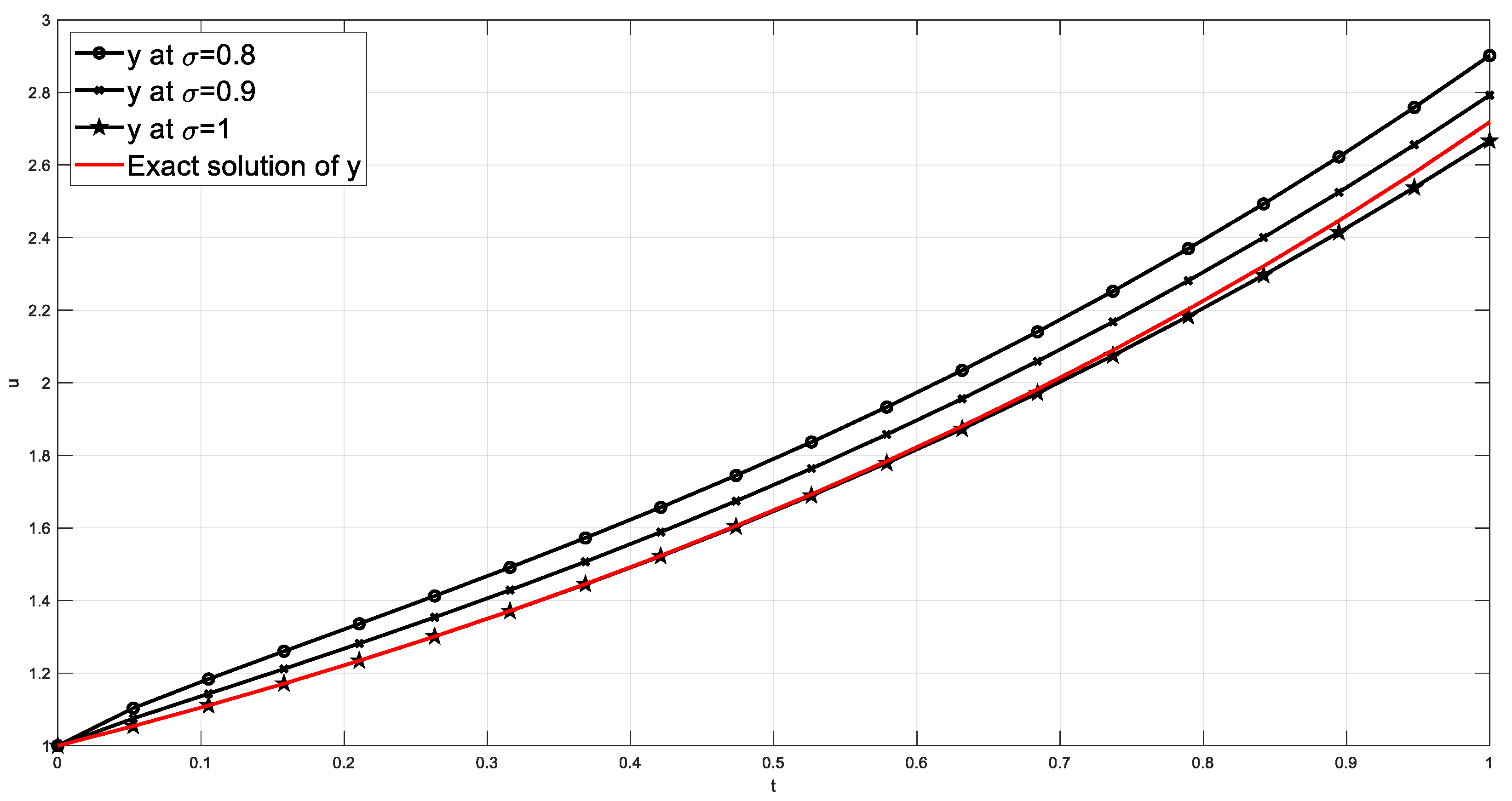
0.1039	1.1818	1.1415	1.1095	1.1095	0.0723	0.0320	0.0000
0.2034	1.3258	1.2721	1.2255	1.2256	0.1002	0.0465	0.0001
0.3030	1.4719	1.4103	1.3536	1.3539	0.1180	0.0564	0.0004
0.4026	1.6267	1.5595	1.4945	1.4957	0.1310	0.0639	0.0012
0.5021	1.7939	1.7220	1.6493	1.6523	0.1416	0.0698	0.0029
0.6017	1.9762	1.8996	1.8191	1.8253	0.1509	0.0744	0.0062
0.7013	2.1761	2.0940	2.0047	2.0164	0.1597	0.0776	0.0117
0.8009	2.3957	2.3066	2.2072	2.2275	0.1682	0.0791	0.0203
0.9004	2.6369	2.5389	2.4275	2.4607	0.1762	0.0782	0.0332
1.0000	2.9016	2.7924	2.6667	2.7183	0.1833	0.0741	0.0516

Table 2. Values of the approximate and exact solutions of Equation (24) at different values of $𝓉$.

$\mathit{t}$	${\mathbf{𝓎}}_{\mathit{\sigma }=0.8}$	${\mathbf{𝓎}}_{\mathit{\sigma }=0.9}$	${\mathbf{𝓎}}_{\mathit{\sigma }=1}$	${\mathbf{𝓎}}_{\mathit{e}}$	$|{\mathbf{𝓎}}_{\mathit{e}}-{\mathbf{𝓎}}_{0.8}|$	$|{\mathbf{𝓎}}_{\mathit{e}}-{\mathbf{𝓎}}_{0.9}|$	$|{\mathbf{𝓎}}_{\mathit{e}}-{\mathbf{𝓎}}_1|$
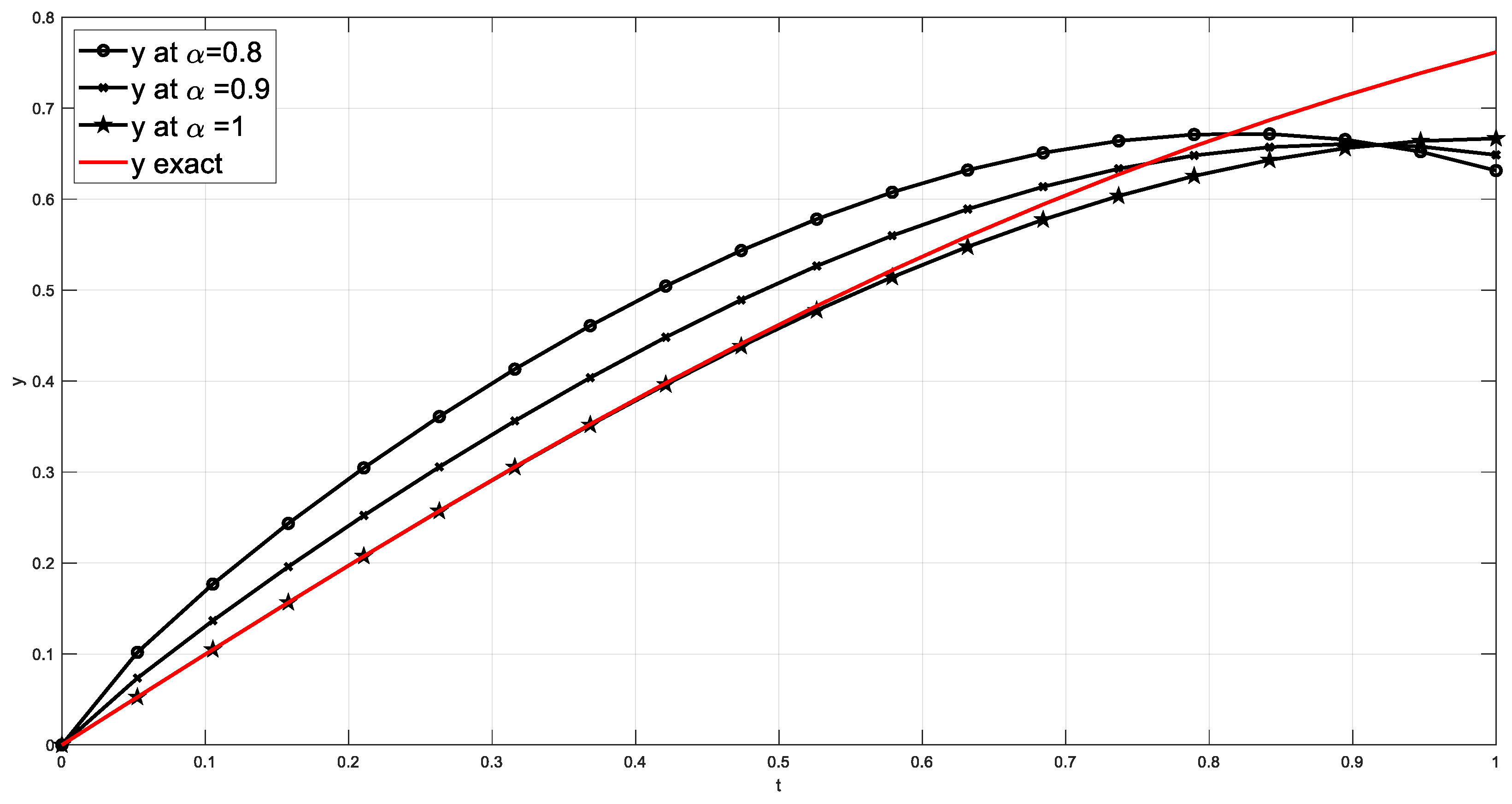
0.1000	0.1697	0.1305	0.0997	0.0997	0.0701	0.0308	0.0000
0.2000	0.2927	0.2411	0.1973	0.1974	0.0954	0.0438	0.0000
0.3000	0.3979	0.3413	0.2910	0.2913	0.1065	0.0500	0.0003
0.4000	0.4875	0.4308	0.3787	0.3799	0.1076	0.0508	0.0013
0.5000	0.5614	0.5083	0.4583	0.4621	0.0993	0.0462	0.0038
0.6000	0.6180	0.5721	0.5280	0.5370	0.0809	0.0350	0.0090
0.7000	0.6555	0.6201	0.5857	0.6044	0.0511	0.0157	0.0187
0.8000	0.6717	0.6503	0.6293	0.6640	0.0077	0.0137	0.0347
0.9000	0.6645	0.6606	0.6570	0.7163	0.0518	0.0557	0.0593
1.0000	0.6314	0.6486	0.6667	0.7616	0.1302	0.1130	0.0949

Table 3. Values of the approximate and exact solutions of Equation (26) at different values of $𝓉$.

$\mathit{t}$	${\mathbf{𝓎}}_{\mathit{\sigma }=0.8}$	${\mathbf{𝓎}}_{\mathit{\sigma }=0.9}$	${\mathbf{𝓎}}_{\mathit{\sigma }=1}$	${\mathbf{𝓎}}_{\mathit{e}}$	$|{\mathbf{𝓎}}_{\mathit{e}}-{\mathbf{𝓎}}_{0.8}|$	$\left|{\mathbf{𝓎}}_{\mathit{e}}-{\mathbf{𝓎}}_{0.9}\right|$	$|{\mathbf{𝓎}}_{\mathit{e}}-{\mathbf{𝓎}}_1|$
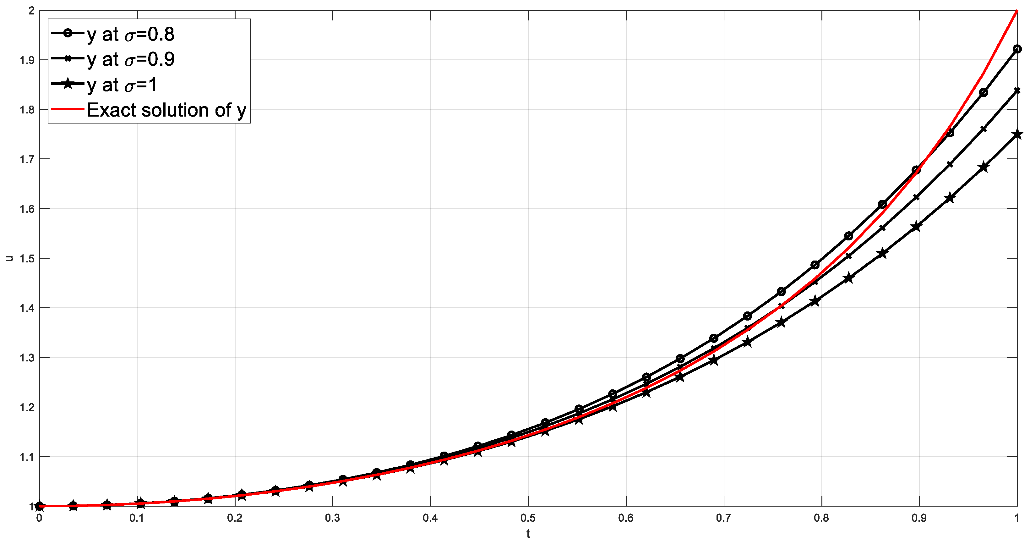
0.1180	1.0073	1.0073	1.0070	1.0070	0.0003	0.0002	0.0000
0.2160	1.0252	1.0248	1.0239	1.0239	0.0013	0.0009	0.0000
0.3140	1.0553	1.0540	1.0517	1.0519	0.0034	0.0022	0.0001
0.4120	1.1000	1.0969	1.0921	1.0927	0.0073	0.0042	0.0007
0.5100	1.1627	1.1561	1.1470	1.1495	0.0132	0.0066	0.0025
0.6080	1.2474	1.2348	1.2190	1.2267	0.0207	0.0081	0.0077
0.7060	1.3593	1.3373	1.3113	1.3319	0.0274	0.0054	0.0206
0.8040	1.5043	1.4682	1.4277	1.4776	0.0268	0.0093	0.0499
0.9020	1.6892	1.6331	1.5723	1.6858	0.0035	0.0527	0.1135
1.0000	1.9218	1.8382	1.7500	2.0000	0.0782	0.1618	0.2500

Table 4. Values of the approximate and exact solutions of Equation (28) at different values of $𝓉$.

$\mathit{t}$	${\mathbf{𝓎}}_{\mathit{\sigma }=0.8}$	${\mathbf{𝓎}}_{\mathit{\sigma }=0.9}$	${\mathbf{𝓎}}_{\mathit{\sigma }=1}$	${\mathbf{𝓎}}_{\mathit{e}}$	$|{\mathbf{𝓎}}_{\mathit{e}}-{\mathbf{𝓎}}_{0.8}|$	$\left|{\mathbf{𝓎}}_{\mathit{e}}-{\mathbf{𝓎}}_{0.9}\right|$	$|{\mathbf{𝓎}}_{\mathit{e}}-{\mathbf{𝓎}}_1|$
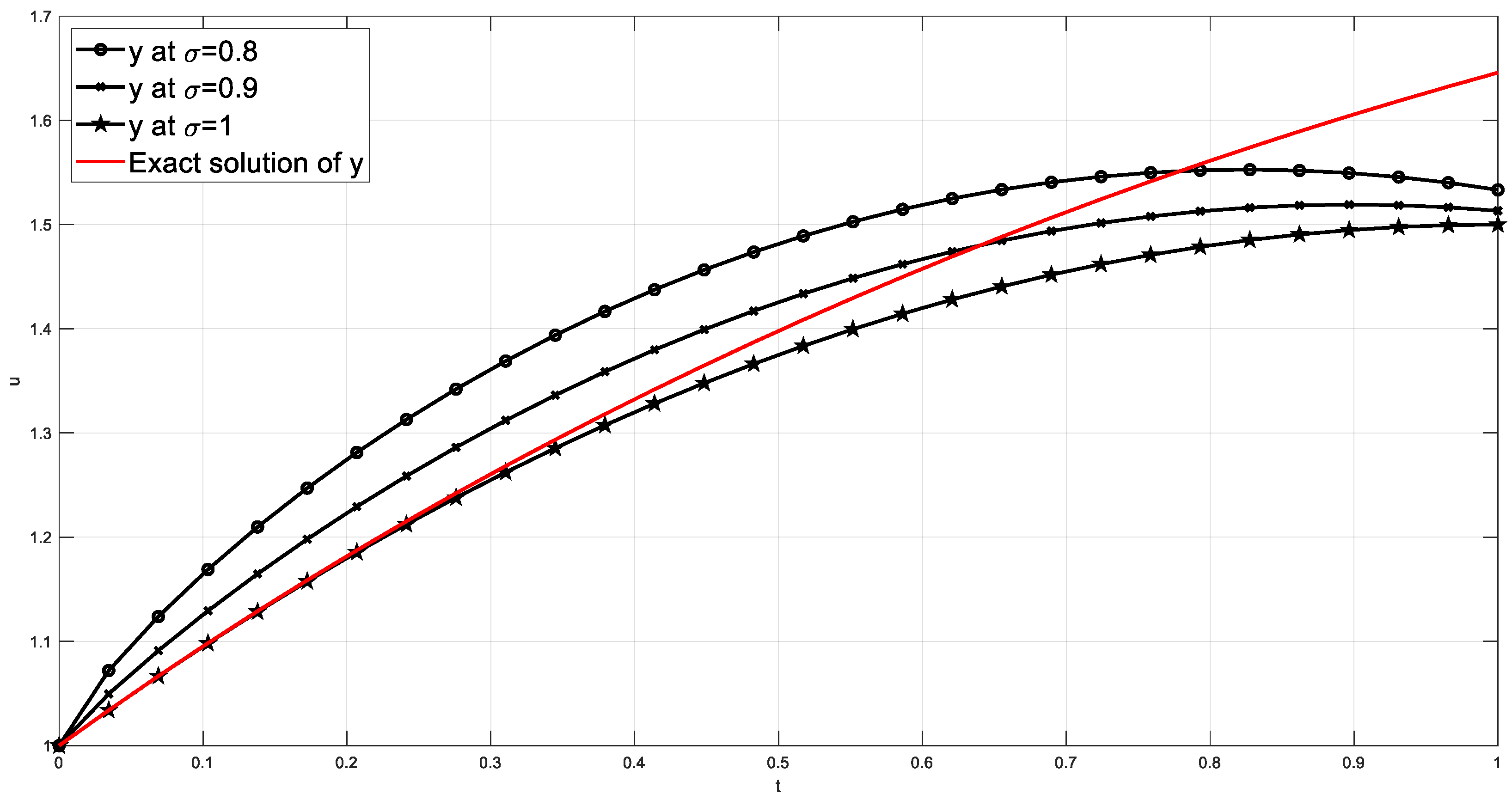
0.1180	1.1867	1.1446	1.1110	1.1114	0.0753	0.0332	0.0004
0.2160	1.2899	1.2372	1.1927	1.1948	0.0950	0.0424	0.0022
0.3140	1.3717	1.3147	1.2647	1.2710	0.1008	0.0437	0.0063
0.4120	1.4365	1.3787	1.3271	1.3406	0.0959	0.0381	0.0134
0.5100	1.4860	1.4302	1.3800	1.4041	0.0818	0.0261	0.0242
0.6080	1.5213	1.4698	1.4232	1.4622	0.0592	0.0076	0.0390
0.7060	1.5433	1.4976	1.4568	1.5151	0.0283	0.0175	0.0583
0.8040	1.5524	1.5140	1.4808	1.5631	0.0107	0.0491	0.0823
0.9020	1.5490	1.5192	1.4952	1.6066	0.0576	0.0874	0.1114
1.0000	1.5333	1.5132	1.5000	1.6458	0.1125	0.1326	0.1458

Figure 1. Approximate and exact solutions of Equation (19).

Figure 2. Approximate and exact solutions of Equation (24).

Figure 3. Approximate and exact solutions of Equation (26).

Figure 4. Approximate and exact solutions of Equation (28).

5. Conclusions

A new approach is proposed for solving fractional ordinary differential equations. The strength of this new method lies in its ability to solve different types of fractional ordinary differential equations, such as linear, nonlinear, homogeneous, and nonhomogeneous, of the order $0<\sigma \le 1$. The results of this study show that the approximate solutions obtained from the proposed algorithm are highly consistent with the exact solutions. Moreover, this method can be developed to solve ordinary differential equations, partial differential equations, integral equations, and fractional differential equations. It is also recommended for solving boundary value problems of differential equations.

References

- Singh, J.; Jassim, H.K.; Kumar, D. An efficient computational technique for local fractional Fokker-Planck equation. Phys. A Stat. Mech. Appl. 2020, 555, 124525. [Google Scholar] [CrossRef]
- Jassim, H.K.; Shareef, M.A. On approximate solutions for fractional system of differential equations with Caputo-Fabrizio fractional operator. J. Math. Comput. Sci. 2021, 23, 58–66. [Google Scholar] [CrossRef]
- Jassim, H.K.; Hussein, M.A. A Novel Formulation of the Fractional Derivative with the Order 𝛼 ≥ 0 and without the Singular Kernel. Mathematics 2022, 10, 4123. [Google Scholar]
- Adomian, G. A new approach to nonlinear partial differential equations. J. Math. Anal. Appl. 1984, 102, 420–434. [Google Scholar] [CrossRef]
- He, J.H. A new approach to nonlinear partial differential equations. Commun. Nonlinear Sci. Numer. Simul. 1997, 2, 203–205. [Google Scholar] [CrossRef]
- He, J.H. Homotopy perturbation method: A new nonlinear analytical technique. Appl. Math. Comput. 2003, 135, 73–79. [Google Scholar] [CrossRef]
- Liao, S.J. Beyond Perturbation: Introduction to the Homotopy Analysis Method; Chapman & Hall/CRC Press: Boca Raton, FL, USA, 2003. [Google Scholar]
- Zhou, J.K. Differential Transformation and Its Application for Electrical Circuits; Huazhong University Press: Wuhan, China, 1986. [Google Scholar]
- Zhang, J.L.; Wang, M.L.; Wang, Y.M.; Fang, Z.D. The improved F-expansion method and its applications. Phys. Lett. A 2006, 350, 103–109. [Google Scholar] [CrossRef]
- He, J.H.; Wu, X.H. Exp-function method for nonlinear wave equations. Chaos Solitons Fract. 2006, 30, 700–708. [Google Scholar] [CrossRef]
- Wazwaz, A.M. A sine–cosine method for handling nonlinear wave equations. Math. Comput. Model. 2004, 40, 499–508. [Google Scholar] [CrossRef]
- Baleanu, D.; Jassim, H.K.; Khan, H. A modification fractional variational iteration method for solving nonlineargas dynamic and coupled KdV equations involving local fractional operators. Thermal Sci. 2018, 22, 165–175. [Google Scholar] [CrossRef]
- Alzaki, L.K.; Jassim, H.K. The approximate analytical solutions of nonlinear fractional ordinary differential equations. Int. J. Nonlinear Anal. Appl. 2021, 12, 527–535. [Google Scholar]
- Jassim, H.K.; Kadhim, H.A. Fractional Sumudu decomposition method for solving PDEs of fractional order. J. Appl. Comput. Mech. 2021, 7, 302–311. [Google Scholar]
- Jafari, H. A new general integral transform for solving integral equations. J. Adv. Res. 2021, 32, 133–138. [Google Scholar] [CrossRef]
- Zayir, M.Y.; Jassim, H.K. A unique approach for solving the fractional Navier–Stokes equation. J. Mult. Math. 2022, 25, 2611–2616. [Google Scholar] [CrossRef]
- Jafari, H.; Zayir, M.Y.; Jassim, H.K. Analysis of fractional Navier-Stokes equations. Heat Transfer 2023, 1–19. [Google Scholar] [CrossRef]
- Alzaki, L.K.; Jassim, H.K. Time-Fractional Differential Equations with an Approximate Solution. J. Niger. Soc. Phys. Sci. 2022, 4, 1–8. [Google Scholar] [CrossRef]
- Jassim, H.K.; Ahmad, H.; Shamaoon, A.; Cesarano, C. An efficient hybrid technique for the solution of fractional-order partial differential equations. Carpathian Math. Publ. 2021, 13, 790–804. [Google Scholar] [CrossRef]
- Fan, Z.P.; Jassim, H.K.; Raina, R.; Yang, X.J. Adomian decomposition method for three-dimensional diffusion model in fractal heat transfer involving local fractional derivatives. Thermal Sci. 2015, 19, 137–141. [Google Scholar] [CrossRef]
- Xu, S.; Ling, X.; Zhao, Y.; Jassim, H.K. A novel schedule for solving the two-dimensional diffusion problem in fractal heat transfer. Thermal Sci. 2015, 19, 99–103. [Google Scholar] [CrossRef]
- Jassim, H.K. Analytical Approximate Solutions for Local Fractional Wave Equations. Math. Methods Appl. Sci. 2020, 43, 939–947. [Google Scholar] [CrossRef]
- Jassim, H.K.; Vahidi, J.; Ariyan, V.M. Solving Laplace Equation within Local Fractional Operators by Using Local Fractional Differential Transform and Laplace Variational Iteration Methods. Nonlinear Dyn. Syst. Theory 2020, 20, 388–396. [Google Scholar]
- Baleanu, D.; Jassim, H.K. Exact Solution of Two-dimensional Fractional Partial Differential Equations. Fractal Fract. 2020, 4, 21. [Google Scholar] [CrossRef]
- Jassim, H.K.; Vahidi, J. A New Technique of Reduce Differential Transform Method to Solve Local Fractional PDEs in Mathematical Physics. Int. J. Nonlinear Anal. Appl. 2021, 12, 37–44. [Google Scholar]
- Jassim, H.K.; Khafif, S.A. SVIM for solving Burger’s and coupled Burger’s equations of fractional order. Prog. Fract. Differ. Appl. 2021, 7, 1–6. [Google Scholar]
- Kumar, D.; Agarwal, R.P.; Singh, J. A modified numerical scheme and convergence analysis for fractional model of Lienard’s equation. J. Comput. Appl. Math. 2018, 339, 405–413. [Google Scholar] [CrossRef]
- Singh, J.; Kumar, D.; Baleanu, D.; Rathore, S. An efficient numerical algorithm for the fractional Drinfeld–Sokolov–Wilson equation. Appl. Math. Comput. 2018, 335, 12–24. [Google Scholar] [CrossRef]
- Jassim, H.K. New Approaches for Solving Fokker Planck Equation on Cantor Sets within Local Fractional Operators. J. Math. 2015, 2015, 684598. [Google Scholar] [CrossRef]
- Jafari, H.; Jassim, H.K.; Baleanu, D.; Chu, Y.M. On the approximate solutions for a system of coupled Korteweg-de Vries equations with local fractional derivative. Fractals 2021, 29, 2140012. [Google Scholar] [CrossRef]
- Jafari, H.; Jassim, H.K.; Vahidi, J. Reduced differential transform and variational iteration methods for 3D diffusion model in fractal heat transfer within local fractional operators. Thermal Sci. 2018, 22, 301–307. [Google Scholar] [CrossRef]
- Wang, K.-J.; Shi, F. A New Perspective on the Exact Solutions of the Local Fractional Modified Benjamin-Bona-Mahony Equation on Cantor Sets. Fractal Fract. 2023, 7, 72. [Google Scholar] [CrossRef]
- Jassim, H.K.; Mohammed, M.G. Natural homotopy perturbation method for solving nonlinear fractional gas dynamics equations. Int. J. Nonlinear Anal. Appl. 2021, 12, 813–821. [Google Scholar]
- Mohammed, M.G.; Jassim, H.K. Numerical simulation of arterial pulse propagation using autonomous models. Int. J. Nonlinear Anal. Appl. 2021, 12, 841–849. [Google Scholar]
- Taher, H.G.; Jassim, H.K.; Hassan, N.J. Approximate analytical solutions of differential equations with Caputo-Fabrizio fractional derivative via new iterative method. AIP Conf. Proc. 2022, 2398, 060020. [Google Scholar]
- Sachit, S.A.; Jassim, H.K.; Hassan, N.J. Revised fractional homotopy analysis method for solving nonlinear fractional PDEs. AIP Conf. Proc. 2022, 2398, 060044. [Google Scholar]
- Mahdi, S.H.; Jassim, H.K.; Hassan, N.J. A new analytical method for solving nonlinear biological population model. AIP Conf. Proc. 2022, 2398, 060043. [Google Scholar]
- Wang, S.Q.; Yang, Y.J.; Jassim, H.K. Local Fractional Function Decomposition Method for Solving Inhomogeneous Wave Equations with Local Fractional Derivative. Abstr. Appl. Anal. 2014, 2014, 176395. [Google Scholar] [CrossRef]
- Yan, S.P.; Jafari, H.; Jassim, H.K. Local Fractional Adomian Decomposition and Function Decomposition Methods for Solving Laplace Equation within Local Fractional Operators. Adv. Math. Phys. 2014, 2014, 161580. [Google Scholar] [CrossRef]
- Abbas, S.M.; Saïd, M.B.; Gaston, M.N. Topics in Fractional Differential Equations; Springer Science & Business Media: Berlin/Heidelberg, Germany, 2012; Volume 27. [Google Scholar]
- Shantanu, D. Functional Fractional Calculus; Springer: Berlin, Germany, 2011; Volume 1. [Google Scholar]
- Podlubny, I. Fractional Differential Equations; Academic Press: San Diego, CA, USA, 1999. [Google Scholar]