Article

Genetics Information with Functional Brain Networks for Dementia Classification

Department of Information and Communication Engineering, Chosun University, 309 Pilmun-Daero, Dong-gu, Gwangju 61452, Republic of Korea
*
Author to whom correspondence should be addressed.
Mathematics 2023, 11(6), 1529; https://doi.org/10.3390/math11061529
Submission received: 25 February 2023 / Revised: 19 March 2023 / Accepted: 20 March 2023 / Published: 21 March 2023

Abstract

:
Mild cognitive impairment (MCI) precedes the Alzheimer’s disease (AD) continuum, making it crucial for therapeutic care to identify patients with MCI at risk of progression. We aim to create generalized models to identify patients with MCI who advance to AD using high-dimensional-data resting state functional magnetic resonance imaging (rs-fMRI) brain networks and gene expression. Studies that integrate genetic traits with brain imaging for clinical examination are limited, compared with most current research methodologies, employing separate or multi-imaging features for disease prognosis. Healthy controls (HCs) and the two phases of MCI (convertible and stable MCI) along with AD can be effectively diagnosed using genetic markers. The rs-fMRI-based brain functional connectome provides various information regarding brain networks and is utilized in combination with genetic factors to distinguish people with AD from HCs. The most discriminating network nodes are identified using the least absolute shrinkage and selection operator (LASSO). The most common brain areas for nodal detection in patients with AD are the middle temporal, inferior temporal, lingual, hippocampus, amygdala, and middle frontal gyri. The highest degree of discriminative power is demonstrated by the nodal graph metrics. Similarly, we propose an ensemble feature-ranking algorithm for high-dimensional genetic information. We use a multiple-kernel learning support vector machine to efficiently merge multipattern data. Using the suggested technique to distinguish AD from HCs produced combined features with a leave-one-out cross-validation (LOOCV) classification accuracy of 93.07% and area under the curve (AUC) of 95.13%, making it the most state-of-the-art technique in terms of diagnostic accuracy. Therefore, our proposed approach has high accuracy and is clinically relevant and efficient for identifying AD.

1. Introduction

Alzheimer’s disease (AD) is a neurodegenerative condition that influences the brain tissue responsible for memory, thinking, learning, and behavioral tendencies. AD is an irreversible progressive disorder that often influences the elderly. Recently, studies on the prodromal stage, sometimes referred to as mild cognitive impairment (MCI), have attracted significant attention. Based on recent studies, the overall prevalence of AD is over 60 million over the previous 50 years [1]. Consequently, numerous studies on AD to comprehend the underlying development and demonstrate the requirement for early, precise diagnosis to slow the progression of AD have been conducted, although the procedure cannot be reversed [2]. MCI and AD can be identified using biomarkers that rely on imaging techniques, such as positron emission tomography (PET), structural magnetic resonance imaging (sMRI), and resting-state functional MRI (rs-MRI) [3]. Moreover, genome-wide association studies (GWASs) have demonstrated that genetic variants, such as single-nucleotide polymorphisms (SNPs), are the inherent causes of AD owing to their aberrant expression in cerebral anatomy and function [4,5]. Accordingly, a multimodal fusion study to examine the relationship between neuroimaging and gene data might represent a revolution in the study of AD.
Functional MRI (fMRI) [6] has been widely employed as an imaging modality in brain research. The blood oxygenation level dependency and real-time in vivo imaging of brain activity using fMRI are beneficial for the production and analysis of hemodynamic changes [7]. More can be learned about aberrant network connections between mental and neurological disorders by examining the functional or structural network topology among patients. Network analysis techniques are widely used to detect brain abnormalities early in life [8,9]. In addition, a high-throughput genotyping method of large-scale population DNA samples was examined in previous studies (GWAS) [10] to detect the gene copy number variation or SNPs, which are high-density genetic markers. This method effectively determines disease susceptibility. Genetic variables significantly influence many aspects of health according to GWAS-based research to evaluate SNPs data for the progression of AD [11,12]. Dukart et al. [13] achieved an efficiency of 76% using Naive Bayes to distinguish between stable and transient MCI using PET as a specific biomarker. The efficiency increased to approximately 87% when integrating apolipoprotein E (APOE) information with imaging data. According to Dukart et al., the inclusion of genetic elements can assist imaging features to achieve higher classification accuracy. Graph theory topological metrics, which are parts of the brain’s functional connectome, have become crucial imaging biomarkers to better understand brain networks and identify neurodegenerative disorders [14,15]. The functional connectome systematically shows that the network’s nodal graph metrics, such as degree, participation coefficient, and shortest path length; global graph metrics, such as small world, modularity, and global efficiency; as well as functional connections among brain regions have disease diagnosis potentials. This offers a novel technique to spot altered brain network patterns [15,16]. Important aspects of brain networks have been chosen using sparse approaches, such as the least absolute shrinkage and selection operator (LASSO), because of the higher number of connectome features in the brain [9]. The LASSO regression analysis approach for feature selection and regularization can be used to choose nodal graph metrics and preserve strong discriminative nodal features [17]. In the recent past, methods to combine and identify brain regions have been developed using data-driven techniques and machine learning algorithms. Support vector machines (SVMs), Naive Bayes [18], and deep neural networks [19] have been used to identify individuals with MCI and healthy controls (HCs) [20]. However, most of these techniques isolate only one modality feature, resulting in poor classification performance. Multimodal characteristics should be utilized to offer a thorough and relevant knowledge of biomarkers in patients with AD. Multiple-kernel-learning SVM (MKL-SVM) [21] can assess the contributions of peculiar biomarkers to classification and partially ease the high-dimensional multiple-features problem.
This study presents research on brain network features and genetic information. The combined analysis of genetic information and brain imaging for predictive identification faces numerous challenges, including computational and statistical issues [22], as well as the heterogeneity of different feature modalities. Similarly, models may run into multicollinearity issues for likely related high-dimensional genetic variables [23], given that genetic features with high dimensions sometimes have redundant information. We use the group-LASSO for brain nodes and ensemble feature selection for genetic information with MKL-SVM to learn genetic information and brain imaging to increase the precision of AD diagnosis and fully utilize the information between various modalities. We also compare the performance of our model with random forest (RF) and extreme gradient boost (XGB) classifiers. The block diagram of the proposed approach is shown in Figure 1.

2. Materials and Methods

2.1. Data

The dataset utilized in this experimental study was collected from the Alzheimer’s disease neuroimaging initiative (ADNI) database, which contains various neuroimaging and genetics datasets. The ADNI collection was accredited by the institutional review board (IRB) for each data collection site. To minimize the potential effects of various image acquisition and genotyping methods, considering the category balance problem, we evaluated participants with brain imaging and genetic data acquired at the same age. Table 1 shows participants’ demographics that were reviewed in detail in this study.

2.2. Data Acquisition

The ADNI (http://adni.loni.usc.edu; accessed on 27 September 2022) provided funding to obtain and distribute data for this investigation. Informed consent was obtained from the volunteers in compliance with the guidelines of the IRB. All techniques were used in compliance with the applicable rules and regulations. In this study, the experimental samples from the ADNI comprised 45 AD patients, 33 MCIs, 35 MCIc, and 32 HC, each of which had resting fMRI and SNP data. There was no significant age difference in the groups. Nonetheless, there was a significant difference in the MMSE and CDR across all group combinations (p ˂ 0.05). It showed that MCIc patients had a greater risk of AD than MCIs. All groups had a male dominance and male-to-female ratio was 54:46.
fMRI images were acquired using a 3.0-T Philips medical scanner and all rs-fMRI imaging modalities were accessed using the ADNI database. The individual subjects were instructed not to think and lie down calmly while scanning to obtain brain fMRI images. The arrangement criteria to obtain the imaging modalities are mentioned below: TE = 30 ms, pulse sequence = GR, TR = 3000 ms, flip angle = 80°, pixel spacing X = 3.31 and Y = 3.31 mm, data matrix = 64 × 64, axial slices = 48, slice thickness = 3.33 ms, and time points = 140 with no slice gap.
The Human 610-Quad BeadChip was used to genotype the data and pre-processing was performed as per the accepted quality assurance and impeachment practices. The SNPs value, which ranges from 0 to 1 or 2, represents the minor allele count. Only a minor portion of SNPs represent significant predictors of dementia and are connected to alterations in specific brain regions, whereas the majority of variants may not be associated with the pathogenesis of the disease. We used SNPs information from the top 54 AD candidate genes provided in previous studies to eliminate the large SNPs features [11,24,25].

2.3. Data Pre-Processing

Data processing assistants for resting-state fMRI (DPARSF) [26] and statistical parametric mapping (SPM12) [27] were used for rs-fMRI pre-processing. To guarantee that the first signal was stabilized and that the participants could adapt to their surroundings, the first 10 time points were not used. The final slice underwent a timing adjustment. A six-parameter rigid-body spatial transformation was used to compensate for the impact of head movement. The middle slice of the testing method was used as a reference point for a realignment study, and none of the participants were disqualified for not satisfying the requirements for head motion confined to less than 3 mm or 3°. Gray matter, white matter, and cerebrospinal fluid were segregated from the converted structural images after each individual structural image was linearly co-registered with the mean functional MRI. Subsequently, rs-fMRI data were concurrently resampled into 3 mm isotropic voxels and spatially adjusted to the MNI space using parameters determined from the normalization of structural images. All normalized fMRI images were smoothed with a 6 mm full-width at half-maximum Gaussian kernel. Linear detrending and bandpass filtering at 0.01–0.1 Hz were used to reduce high-frequency physiological noise and low-frequency drift.

2.4. Construction of Graph Matrix

We examined the graph theory morphological characteristics of brain functional networks using the graph theoretical network analysis toolbox (GRETNA) [28] based on statistical parametric mapping (SPM12) and MATLAB R2021a based on binary undirected matrices. The brain connectivity network was built using the average time series for each area based on the automated anatomical labeling (AAL) atlas [29]. The implementation of separate coefficients of Pearson correlation for every pairing of the 90 regions of interest (ROIs) resulted in the definition of the edges of functional links. Consequently, an adjacency matrix (functional connectivity matrix) was created. N, the number of nodes in the network, was translated into N(N − 1)/2 edges in the final functional connection networks. We limited the study to positive correlations by setting zero to a negative correlation because of its unclear interpretation. A thresholding approach based on network sparsity was used to eliminate minor connections while preserving the topological characteristics of graph theory by choosing a proper threshold value for network sparsity [30]. The sparsity criteria were set to acquire a binary undirected network. In our proposed methodology, we only applied the nodal graph matrix, such as the betweenness centrality, nodal clustering coefficient, degree centrality, nodal efficiency, nodal local efficiency, and nodal shortest path. The modularity ( W ) of a brain network measures how effectively a network can be divided into modules [31]. The utilization of an improved greedy optimization approach is shown in Equation (1):
W = d = 1 M n [ e d / E ( s d / 2 E ) 2 ]
where E denotes the total number of networks of edges in the brain, e d is the number of within-module edges in module d , and s d is the sum of the connected edges at each node inside module d . The modular structure was discovered using modified greedy optimization. The following formulas were used to compute the intra-module connection density C d and inter-module connectivity density C d , t at the module level:
C d = 2 i , j ϵ d ε i , j N d ( N d 1 )
where i and j represent the nodes, ε i , j are the edges between node i and j within the d module, and N d represents the overall nodes in module d .
C d , t = i ϵ d , j ϵ t ε i , j N d × N t
N d stands for the number of nodes inside module d , N t represents the number of nodes inside module t , and ε i , j represents the edges connecting module d and t . Here, i and j represent the corresponding edges for nodes i and j . The following metrics were used to assess the participation coefficient (PC) and within-module degree ( M D ) at the nodal level:
M D i = x i x d ¯ σ d
where x i denotes the nodal degree of node i inside module d , x d ¯ represents the regular node degree for all nodes in d , and σ d denotes the standard deviation for the node degree for all nodes in d within the module.
P C i = 1 d = 1 M n ( k i , d k i ) 2
where i represents the number of nodes in brain networks, which means that, in our case, we used the ALL 90 atlas, a 90-region server, as the brain node in our model; Pearson’s correlation [28] was used to define the edge among those ROIs; similarly, d represents the number of modules in brain networks. A brain network’s nodes are often arranged in modules, which means that nodes from the same module are strongly linked to one another while nodes from different modules are sparsely linked [32,33]. The number of connection link between nodes i and d is k i , d , and M n is the number of modules. The link between node i and every other node within M n is a representation of these connections k i .

2.5. Features Selection

The main objective of feature selection is to determine a few key features from the feature pool that will increase diagnostic accuracy. We used the group-LASSO [17] method for the nodal graph matrix and ensemble for genetic features that combines the feature subsets produced from various filters utilizing feature classes with those selected using various feature selection techniques (Chi-Square, InfoGain, and ReliefF) [34]. A brief explanation of each feature-selection method is provided below.

2.5.1. Group Least Absolute and Shrinkage Selection Operation

The relevant feature set was chosen using the group-LASSO, which is a dynamic process [35]. This technique relies on feature reduction and regularization. The 90 AAL functional region atlases were used to partition the brain into 90 nodes. The group topology of the nodal graph metrics easily follows from the fact that each node corresponds to a set of node graph theoretical properties. This method employed the group-LASSO as the feature selection strategy for nodal graph metrics, given the group characteristics.
m i n w i = 1 N l o g ( 1 + e x p ( a i × ( j = 1 n k = 1 m w ( j , k ) , b ( j , k ) + c ) ) ) + λ j = 1 n w j , k q
where w ( j , k ) and b ( j , k ) represent the weight and value for the j th region of interest and k th nodal matrix, respectively; a i is the label of the i th participant. b ( j , k ) was balanced using Fisher Z-transformation to prevent scale imbalance. With the default value of λ = 1 , we calculated w ( j , k ) using [36].

2.5.2. Chi-Square

This feature’s ranking method measures each feature’s chi-squared statistic in relation to the class to determine the significance of each feature; the greater the chi-squared, the more significant the feature for the particular job [37].

2.5.3. InfoGain

InfoGain uses the entropy theory [38]. To reduce the uncertainty level in the classification task, a weight was produced for each variable by estimating the extent to which class entropy decreased when the value of that characteristic was known.

2.5.4. ReliefF

The ReliefF feature selection determines how well the features can distinguish between data points that are close to one another in the attribute space [39]. Essentially, a sample instance is selected from the dataset and its feature values are compared to those of one (or more) of its nearest neighbors for each class. Subsequently, based on the presumption that a “good” feature should have the same value for examples from the same class and different values for instances of different classes, a relevance score is provided for each feature. An appropriate number of sample examples are considered iteratively and the scores for the characteristics are updated accordingly.

2.6. Random Forest Classifier

The random forest (RF) model is a decision-tree-derived ensemble tree-based learning system. To assess the link between independent and dependent variables, the RF method averages predictions over numerous individual trees. Instead of using the original sample, the individual trees are constructed using bootstrap samples. This process, known as bootstrap aggregating, aids in preventing overfitting throughout the model generation process [40].

2.7. Extreme Gradient Boosting Multi-Classifier (XGB) Classifier

As a decision tree’s natural extension, XGB incorporates multiple decision trees to determine the result rather than relying just on one. It can be used for problems involving supervised learning, such as regression, classification, and ranking [41].

2.8. SVM Classifier

The SVM [21] divides the classification group using the best hyperplane as a supervised learning approach. SVM can learn in a certain feature space using training data. Subsequently, the test dataset is categorized according to its organization in the n-dimensional feature space. The SVM is a highly reliable machine learning algorithm in neuroscience and has been used in several neuroimaging applications [22,23]. A linearly separable feature vector can be mathematically divided into lines in a 2D field. The line equation is represented by y = a x + b . The equation becomes a ( x 1 x 2 ) + b = 0 by substituting x with x i and y with x 2 . If we specify x = ( x 1 , x 2 ) and w = ( a 1 ) , we obtain w . x + b = 0 , which results in the hyperplane equation. As in Equation (7), a hyperplane is represented as follows:
f ( y ) = z T ( y ) + b
where y denotes input data, z T denotes a hyperplane, and ( y ) represents a function that maps a vector y into a higher dimensionality. Equation (7) remains unchanged if z and b use equal values to scale correctly. A hyperplane can also provide an exclusive pair ( z , b ) to make any decision boundary, represented as follows:
m i n | z T ( y i ) + b = 1 , i = 1 , 2 , , N . |
where y 1 , y 2 , , y N represents the training features. The hyperplane in Equation (8) is considered canonical. A given hyperplane is expressed as follows:
z T ( x ) + b = 0 ,   w h i c h   i s   s a m e   a s   z T ( y ) = 0 ( w h i c h   h a s   m o r e   d i m e n s i o n s )
Based on Cortes and Vapnik (1995) [42], the equation below indicates a vector x that is not suitable for this hyperplane:
z T ( x ) + b = ± s z
where s represents the vector value corresponding to x for hyperplane representation. Consequently, the distance s ( x ) and z vector for the resulting hyperplane are exactly similar to the output vector f ( y ) from the SVM. Additionally, this study used the kernel-support vector approach, which can effectively handle nonlinear problems using the linear classification method and swaps a linearly unclassifiable vector into a linearly classifiable vector. The intended notion is a vector that is linearly unclassifiable in low dimensions but may be linearly classifiable in high dimensions. The kernel is mathematically expressed as follows:
K ( x , y ) = ( x , y ) d
where x and y represent the features in the input. d represents the kernel parameter. The Gaussian radial bias functions are represented as follows:
K ( x , y ) = e x p ( x y 2 2 σ 2 )
where x and y represent two input samples and x y 2 is the Euclidean distance between two features as a square distance.
Multi-kernel learning (MKL) [43], which enables various kernel functions to represent various subsets of features, broadens the scope of the SVM theory. The multi-kernel SVM [21] approach was used to separate AD cases from controls. The standard SVM, on which our multi-kernel SVM was based, merged several kernel functions linearly before training an SVM classifier using the fused kernel. Equation (13) defines the fused kernel function as a linear combination of fundamental kernels [44].
K ( x i , x j ) = w 1 K 1 ( x i , x j ) + w 2 K 2 ( x i , x j ) + w 3 K 3 ( x i , x j )
where K ( x i , x j ) is the equivalent fundamental kernel and w is its weight. Similarly, K 1 , K 2 , K 3 represent the distinct kernel function. We chose fundamental kernels, such as linear, polynomial, and radial basis functions, to formulate the final kernel function. Equation (14) represents the decision function [42] in the classification:
f ( x ) = s g n { i = 1 n α i × y i d K ( x i , x j ) + b }
where × is the dot product of the vector and i is the Lagrange multiplier. sgn is a representation of a symbolic function connected to a class label. In the linear equation, y i is the expected outcome and b is the intercept. Only two output values exist for the decision function f ( x ) : 1   and + 1 .

2.9. Evaluation Matrices

This study used LOOCV with the MKL-SVM classifier to increase the diagnostic precision for Alzheimer’s detection. Accuracy, specificity, sensitivity, and receiver operating characteristic (ROC) curves were generated to assess the classification performance. A plot of the true positive vs. the false positive rate resulted in the ROC, which assessed the ability of a binary classifier to diagnose problems. The area under the curve (AUC), as assessed by ROC, was negatively associated with the classifier’s performance. Moreover, we measured Cohen’s kappa values for each classification group [45], which measure the inter-rater reliability between the two individuals. Kappa calculates the proportion of information scores in a table’s major diagonal and modifies these scores to account for the amount of agreement that may be inferred from chance only. Cohen’s kappa is determined using Equation (15), where pe is the percentage of observed agreement among raters and po is the fictional chance of random agreement. The Kappa coefficient never exceeded 1. Scores below 1 indicate less than the best agreement, whereas scores of 1 indicate full agreement. Exceptionally, Kappa might have received a poor grade. Thus, two groups agreed less than would be expected by chance.
LOOCV is a widely used data shuffling and resampling method to assess the generalization notion for a predictive model design and to avoid the under or overfitting of classifiers. Predictive modalities, such as classification, frequently employ LOOCV. To address this type of problem, a framework is adjusted using a known dataset, which is sometimes referred to as the training set, and an unknown feature set is assessed using the model as the test set. The objective is to develop a testing sample for the model while still in the training phase and to subsequently show how the model can be adapted to diverse unknown datasets. Multiple divisions employ various LOOCV phases to reduce variability and the average of the findings is considered. LOOCV is a reliable method to assess model performance. The classifiers’ performance in this study was validated using ROC curves. In this method, HC is referred to as negative samples, patients with AD as positive samples, true positives (TP) as the number of positive samples that are correctly categorized, false positives (FP) as the number of negative datasets classified as positives, true negatives (TN) as the number of positive datasets classified as negative, and false negatives (FN) as the number of positive datasets classified as negative samples. The following formula applies to the term’s accuracy, specificity, and precision:
K = p 0 p e 1 p e
A c c u r a c y = T P + T N T P + F P + F N + T N
S p e c i f i c i t y = T N T N + F P
S e n s i t i v i t y = T P T P + F N

3. Results

We assessed the effectiveness of the method through experiments across various cognitive-level healthy versus Alzheimer’s and mild cognitive impairments, which are convertible after certain periods with non-convertibility. We utilized a multi-kernel SVM, RF, and XGB with LOOCV to evaluate the model design in our experiments. MKL-SVM is a classic but powerful machine learning algorithm for disease diagnosis because of the limited number of datasets. First, we constructed brain functional networks from rs-fMRI to examine the distinguishing characteristics of the nodal graph metrics for disease diagnosis.
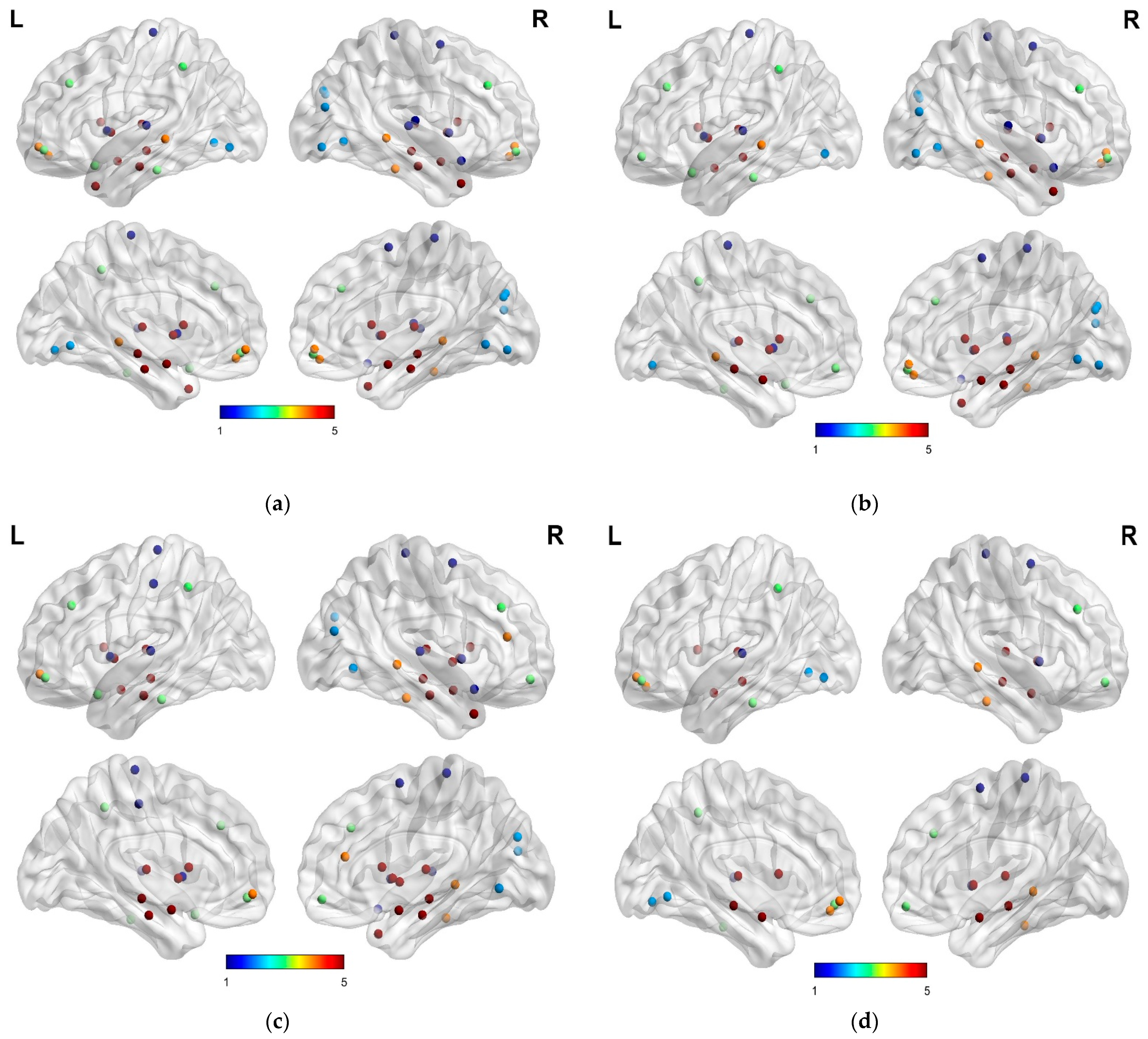
The combination of genetic data and brain imaging has recently gained increasing attention. Brain imaging genomics conducts a complete analysis of genetic information and brain imaging data to generate new insights that can enhance our comprehension of brain functions influenced by diseases. The most discriminating brain areas and SNPs must be identified for an accurate diagnosis of AD. Potential biomarkers for clinical diagnosis can be derived from SNPs data and brain areas that were mostly used in the experiment. As shown in Table 2, we used 54 susceptibility loci found in a recent AD GWAS or GWAS meta-analysis [11,24] in our proposed methodology. We retrieved SNPs matching the requirements below using PLINK v1.9 [46]: by a recent AD GWAS or GWAS meta-analysis with genotyping call rate >95%, Hardy Weinberg Equilibrium > 1.00 × 10⁶, and minor allele frequency >5%. We ran a GWAS (linear regression) in PLINK for each group based on the results collected including variables such as age, gender, and education. We created genetic characteristics for each group using the 54 genes [24] linked to AD. To build a matrix, we first chose the top 54 SNPs for each gene. The matrix was then created using the associated p-values of the SNPs. Each person has a unique brain that varies in size. Associated with extreme values, we used the Min-Max [47] normalization strategy based on this consideration. After that, we corrected the findings of numerous tests using the Bonferroni method. Further, we analyzed 54 AD-related genes and their corresponding loci using the feature-ranking technique, as shown in Figure 2, to access relevant GWAS features. The distribution of various brain network nodes for various classification groups that were consistently chosen in our experiments is shown in Figure 3. Individuals’ memory functions are mostly accessed by the hippocampal and amygdala regions. Thus, these regions are fundamental biomarkers for cognitive decline and can assist in the early diagnosis of AD, and hippocampal network regions serve as crucial prospective biomarkers in the identification of HC in the three phases of the disease condition. Amygdala networks were also used as parameters in the early diagnosis of HC and MCI. This is because, during AD development, network disruption first occurs in the hippocampus and amygdala. In addition, the precentral, cuneus, and inferior parietal lingual network nodes were used in other classification groups. Our findings agree with state-of-the-art methods, which employed an intrinsic brain-based CAD system to identify essential brain areas linked to AD [48]. The AOPE gene is where SNPs that have been repeatedly chosen to classify AD and HC originate from a genetic perspective. As previously mentioned, different parts of brain network nodes are crucial in disease identification and are the most significant risk factors for the development of AD. Two approaches were devised to examine the distinguishing characteristics of nodes based on regional network parameters and nodal graph metrics. On the one hand, we examined the brain networks that were most often used and had the most significant variations in nodal graph metrics. The AAL 90 atlas was used to designate the node positions in individual rs-fMRI brain imaging. From the feature selection using the group-LASSO, among the 90 ROIs, we selected the most significant nodal graph metrics as inputs. Forty-four ROIs were observed to be the most important nodes to separate patients with AD from HC; each ROI had approximately four to seven nodal topological measures that differed significantly from the others. Moreover, we used feature selection as a group-LASSO to identify the distinctive characteristics of each nodal graph attribute. Therefore, cingulate, temporal, superior frontal, parietal gyri, and lingual regions, which correspond to the default mode network, cingulo-opercular network, and dorsal attention network, were the most prevalent brain regions with the discriminatory nodal graph features and more relevant node graph metrics. These ROIs were thought to be the most dominant nodes to separate patients with AD from HC as well as patients with MCIs from MCIc. Consequently, the temporal, superior frontal, parietal gyri, cingulate, lingual, hippocampus, amygdala, and cingulo-opercular regions showed the highest significance for AD vs. HC classification, as shown in Figure 3a. For MCIs vs. MCIc, the hippocampus, amygdala, inferior temporal gyrus, caudate, insula, and paracentral lobule were the most prevalent brain regions with the highest-significance nodal graph features, as shown in Figure 3d. Similarly, for AD vs. MCI classification, the hippocampus, amygdala, lingual, putamen, temporal, and parietal lobules showed the highest significance. Based on additional comparisons of the aforementioned dominant brain parts, individuals with MCI had significantly lower values for degree and betweenness centrality as well as typically larger values for nodal shortest path in the frontal lobe, for example, temporal lobe, bilateral superior frontal gyri, limbic lobe, bilateral inferior temporal gyri, left median cingulate and paracingulate gyri, and parietal lobe. However, the MCI group had considerably lower values of nodal shortest path and significantly higher values of betweenness and degree centrality in the occipital lobe, which contrasted the agreement of the nodal graph in various brain regions.
The AOPE gene is a source of SNPs that is widely used to identify various diseases. In our experiment, these SNPs were determined to be the top contributors, followed by CR1, PVRL2, and CASS4 in order of importance. APOE is associated with disorders that can be measured via neuroimaging, particularly those that influence default mode networks. We performed an ensemble feature selection algorithm for the SNPs in each group as shown in Figure 4. Our analysis revealed the most significant pathogenic genes related to diseases and showed that risk genes, such as PVRL2, CASS4, GPR141, CR1, and INPP5D, were strongly linked to AD. Additionally, these genes are known to be associated with cognitive impairment. CR1 primarily influences AD progression by influencing deposition, changes in brain shape, and glucose metabolism. Many SNPs from the same gene, including CR1 and CASS4, were chosen during the experiment. Our results agree with those of previous studies and aid in the clinical diagnosis and future investigation of AD.
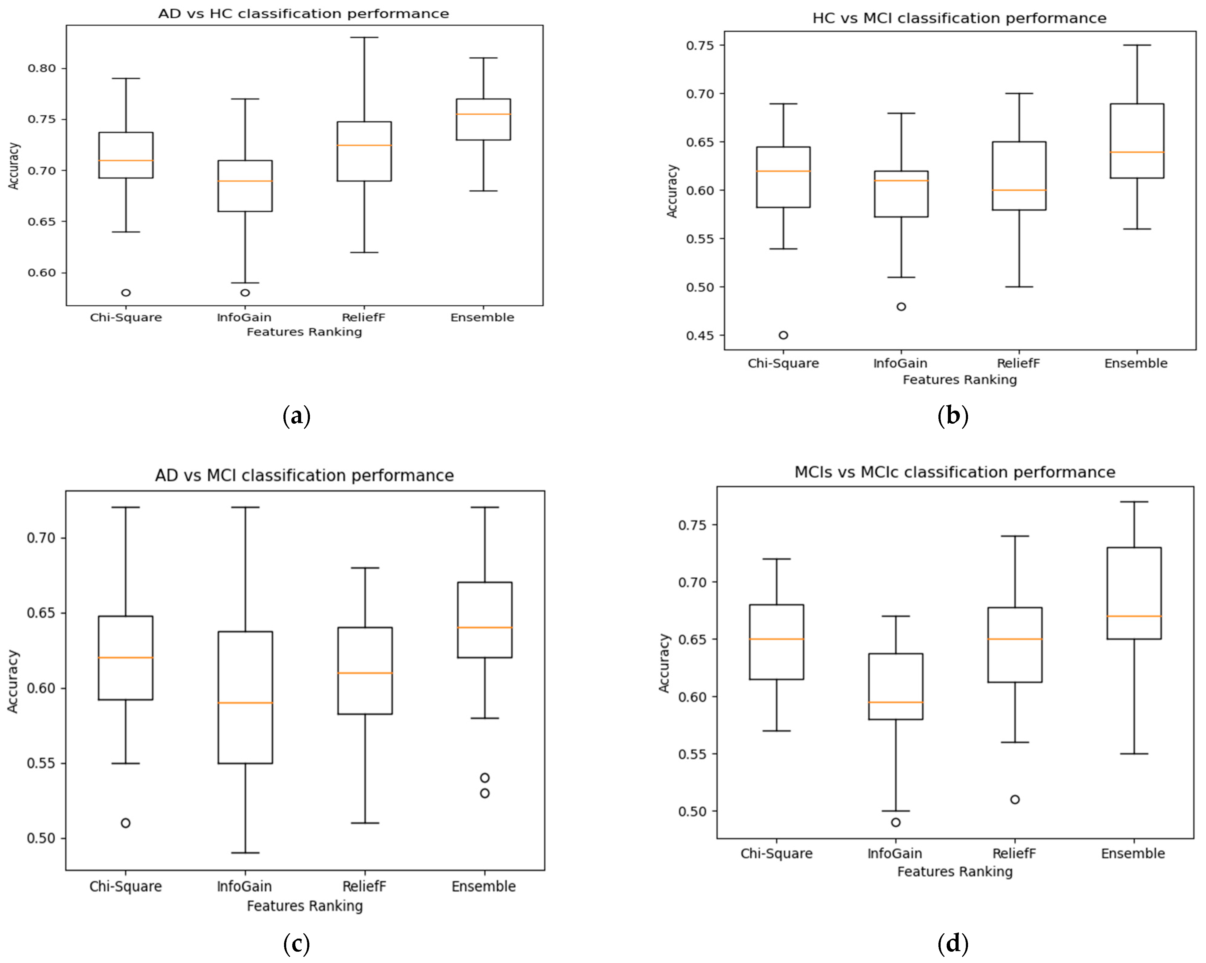
After obtaining the most prevalent brain node and SNPs features, we analyzed the performance of the individual feature set with the combined multi-mode feature set. Because genetic features are high-dimensional, we proposed ensemble feature ranking algorithms to select the important SNPs feature sets. The ensemble feature ranking outperformed the individual feature ranking algorithms. This study used genetic information (SNPs) and network nodal characteristics obtained from rs-fMRI to perform classification analysis. The MKL-SVM classifier with integrated feature methodologies exhibited the highest performance accuracy, although, in some cases, XGB outperformed the MKL-SVM. Overall, the performance of MKL-SVM classifiers was better among the others. The nodal matrix outperformed SNPs because changes in brain connectivity are phenotypic characteristics that are closely associated with diagnostic categories. However, the model’s performance was enhanced compared with using either brain networks or SNPs features by including both genetic and brain network node factors as model predictors. The performance of integrating genetic and imaging data was superior to that of a single modality, particularly when classifying MCI as convertible with stable MCI.
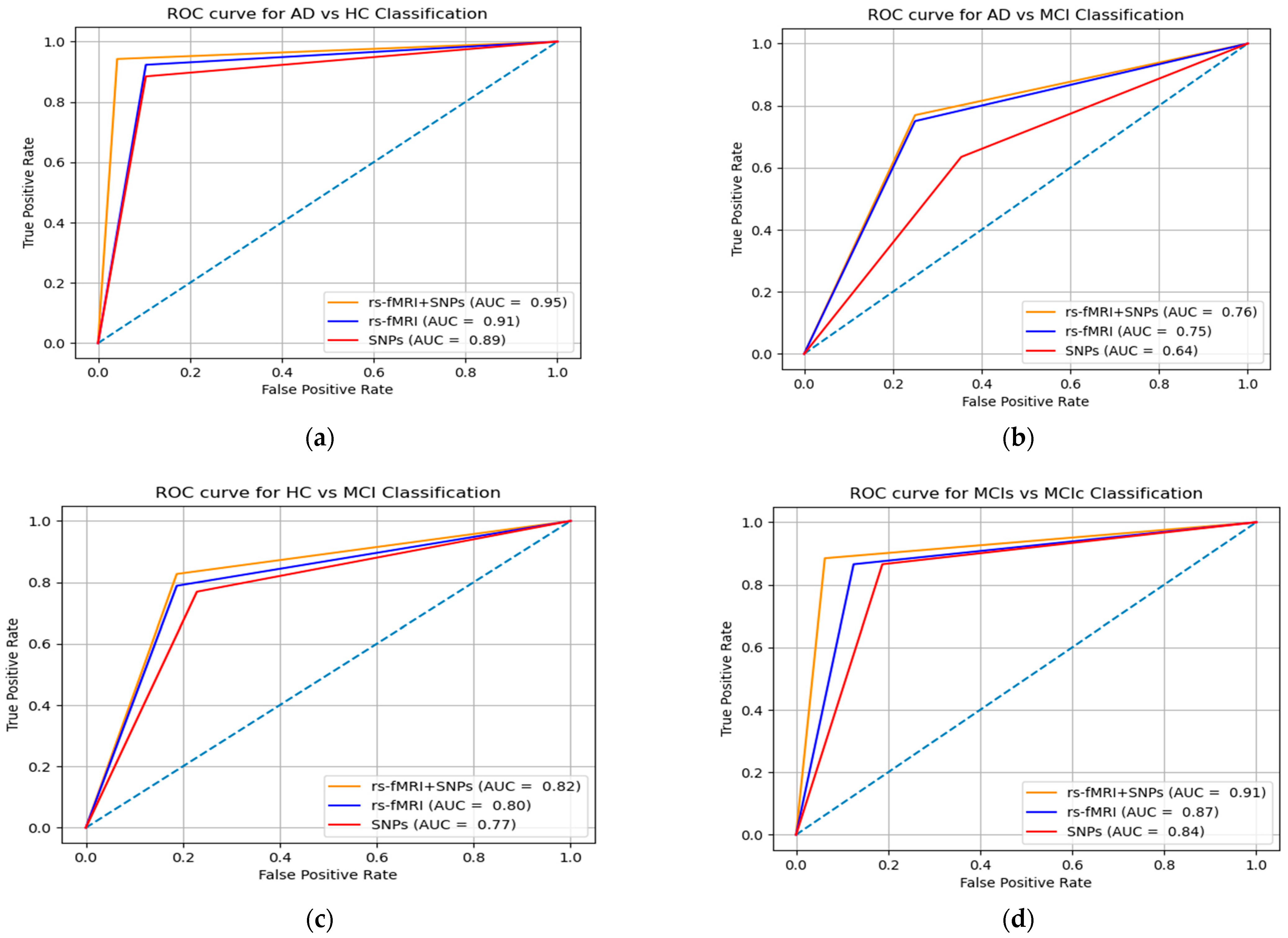
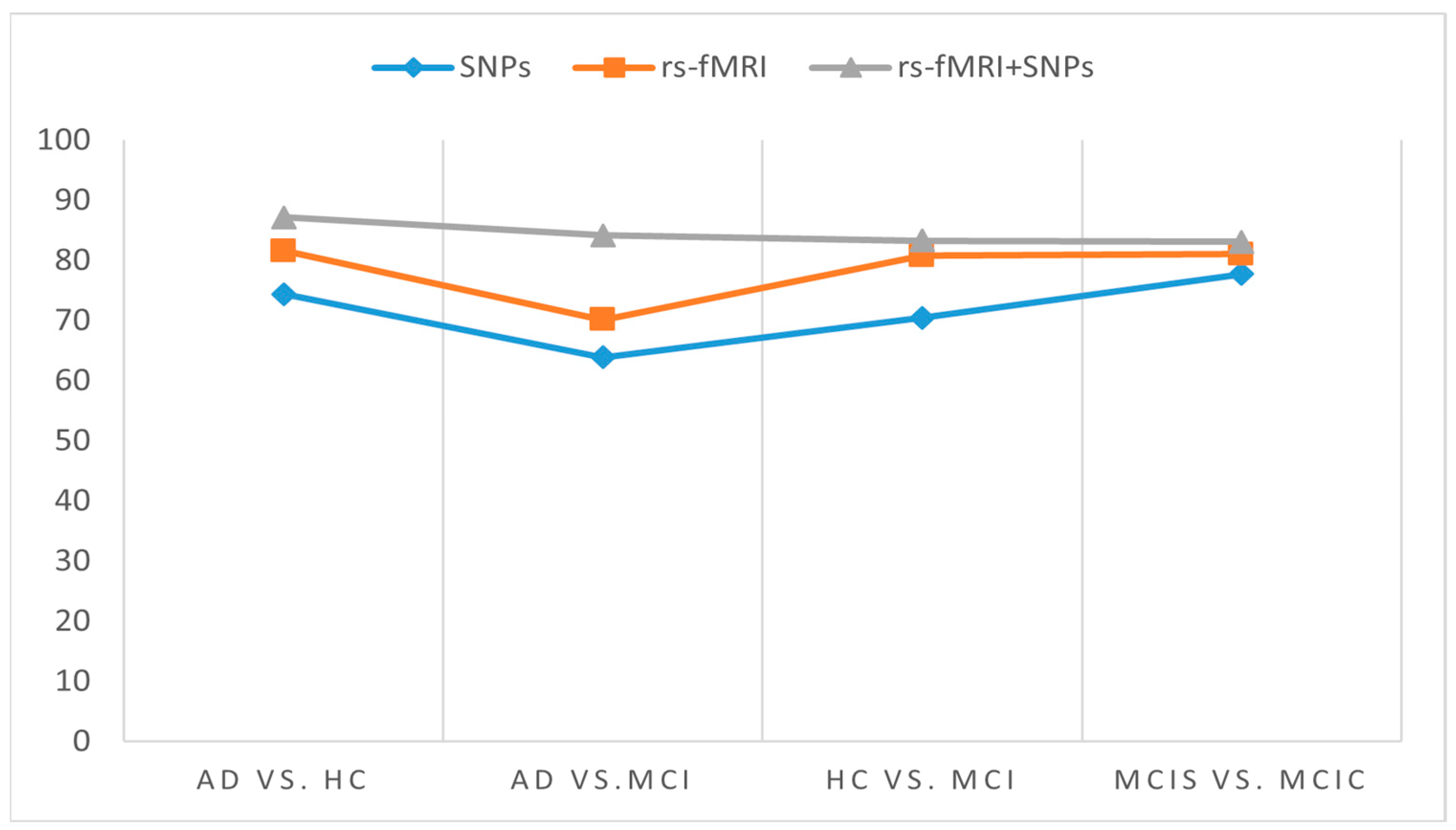
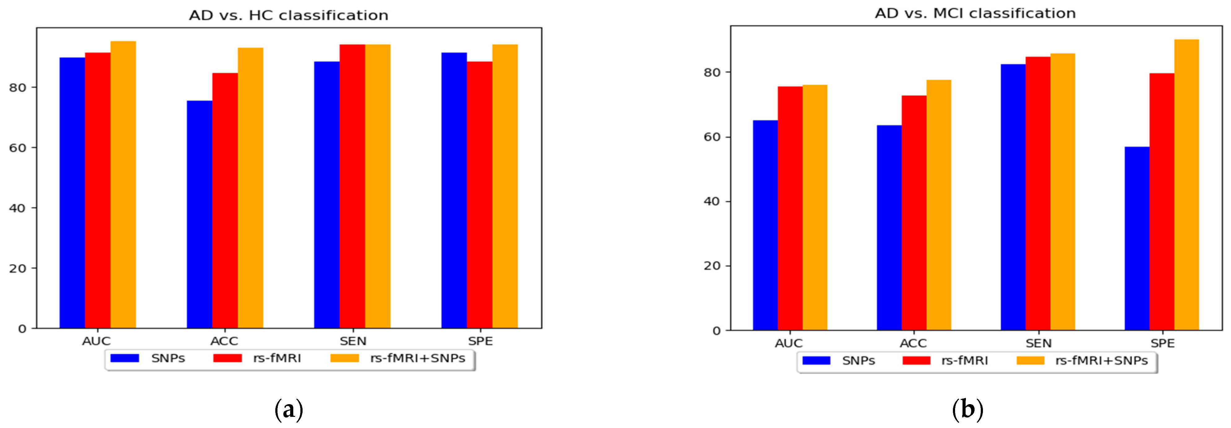
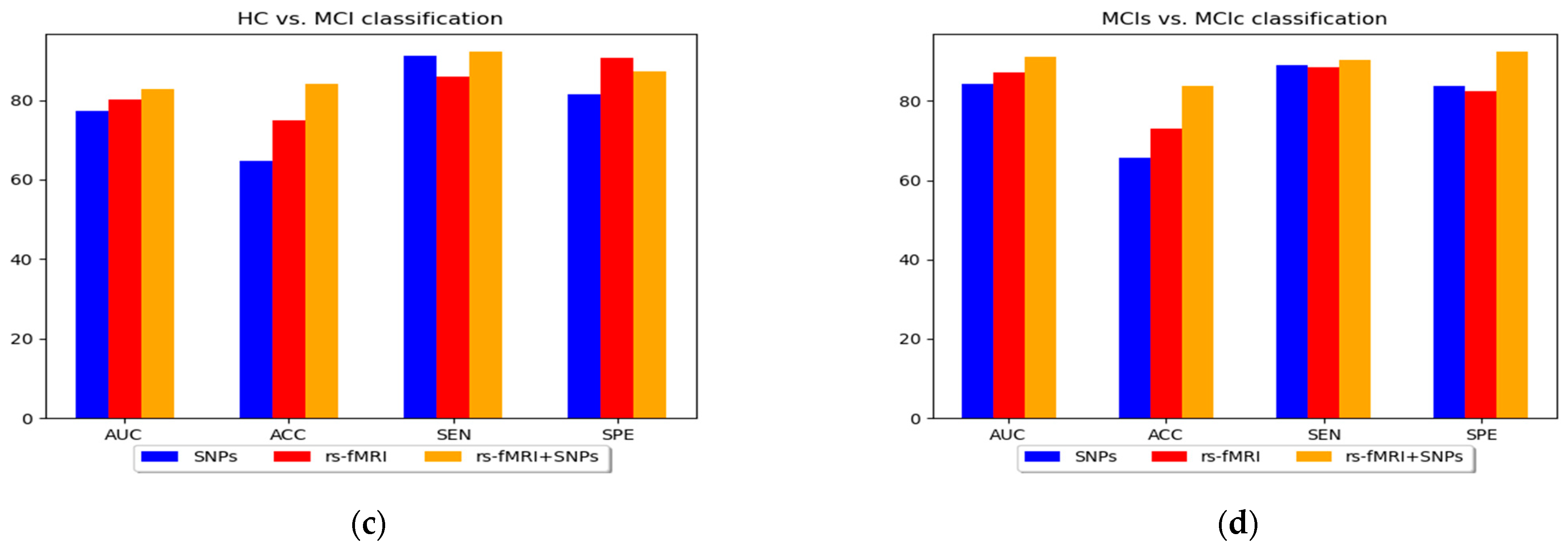
The specificity and sensitivity in Table 3 and the AUC shown in Figure 5 were determined to assess the effectiveness of the MKL-SVM classifier among RF and XGB using the combined feature vectors. Our classification process using brain nodal networks and SNPs feature combinations produced the best performance with 93.03% accuracy, 95.15% sensitivity, 94.17% specificity, 87.17% Cohen’s kappa, and 95.13% AUC for AD vs. HC classification. Similarly, for the MCIs vs. MCIc classification, we obtained 83.73% accuracy, 90.31% sensitivity, 92.37% specificity, 83.09% Cohen’s kappa index, and 91.07% AUC. For the AD vs. MCI classification, we obtained 77.43% accuracy, 85.75% sensitivity, 90.01% specificity, 76.00% AUC, and 84.15% Cohen’s kappa index. Similarly, for the HC vs. MCI classification, we obtained 84.01% accuracy, 92.13% sensitivity, 87.17% specificity, 82.79% AUC, and 83.31% Cohen’s kappa index, as shown in Figure 6. Overall, MKL-SVM exhibited a better performance, but for AD vs. MCI classification on rs-fMRI features, there was a similar performance accuracy with RF and XGB.

4. Discussion

In this study, we constructed and implemented a framework to diagnose AD and its prodromal stage, known as MCI, utilizing SNPs genetic and functional brain networks. Although SNPs genes have complex patterns, a vast field of disease analysis shows the potential for AD identification as complementary features for imaging modalities and assists in increasing model performance. The maximum accuracy was 93.03% and 95.13% AUC for AD vs. HC classification. The use of only SNPs had the lowest performance accuracy when compared with brain network features; however, the performance accuracy of the model was improved when combined with network characteristics. Similarly, we obtained the highest accuracy with feature combinations for AD vs. MCI and HC vs. MCI with 77.43% accuracy and 76.00% AUC, and 84.01% accuracy and 82.79% AUC, respectively. Furthermore, for the AD vs. MCI classification, no significant improvement in model performance was observed with genetic data compared with the network feature set from the results in Table 3 and Figure 7. Therefore, the use of only genetic data was insufficient but, when combined with network features, produced a more accurate categorization result. Furthermore, we combined all the selected network features obtained from rs-fMRI and SNPs and achieved a better classification accuracy compared with the individual features set for all classification groups with the ensemble and group-LASSO feature selection method, as shown in Table 3. In summary, this study elucidated the diagnosis of AD and validated that functional network measurements and genetic tests could be used to identify people with disease conditions. The topmost discriminative features from rs-fMRI brain networks, where each region corresponds to a nodal feature, are shown in Figure 3. In agreement with previous studies, connection anomalies were significantly influenced in the temporal lobe, including the hippocampus, amygdala, mid-temporal, fusiform and inferior temporal, and parietal-occipital regions in the AD vs. HC group. The network connectivity showed a similar pattern for the other two groups, AD vs. MCI and HC vs. MCI, as shown in Figure 3. In conclusion, the highly sensitive brain node observed that the characteristics selected in the experiment utilizing the group-LASSO algorithm had potential. Furthermore, certain brain regions include more disease information with highly sensitive characteristics, allowing for more accurate categorization. The significance of temporal regions, superior frontal, lingual, and parietal gyri in AD diagnosis is generally acknowledged. We recommend that other researchers investigate its function in AD detection.
Moreover, neuroimaging methods for discriminative classification of AD and MCI have been previously analyzed. Most studies used various datasets and classification techniques, both of which significantly influenced the performance accuracy, enabling the comparison with most challenging state-of-the-art methods. As shown in Table 4, the accuracy of several ranges for AD and MCI classification is reported from the binary classification of previous studies in combination with distinct feature selection and various classifiers.

5. Conclusions

First, we examined SNPs and functional network characteristics from rs-fMRI data obtained using ADNI core laboratory biomarkers. The accuracy of numerous computer-aided diagnostic approaches is poor because of the overlap in the data between early brain shrinkage in patients and normal aging in healthy individuals. This study considered both imaging and genetic characteristics as potential classifying factors in this study. Patients with MCIs, MCIc, and AD could be more precisely recognized from HC by efficiently combining consistent brain imaging and genetic information using techniques such as ensemble feature ranking and group-LASSO feature selection with MKL-SVM. Combining SNPs with functional brain networks indicated the possibility of the early detection of AD. We fed the combined kernel matrix into the MKL-SVM classifier using LOOCV cross-validation to obtain the classification result. Moreover, we reported the classification performance in various evaluation matrices, and compared the model performance with RF and XGB classifiers validating the potency of the proposed method for the enhancement of classification performance. In the future, we intend to incorporate a longitudinal dataset, increase the number of datasets, expand the multi-network and multimodal dataset, and utilize other network analysis approaches for rs-fMRI in addition to other feature selection methods to increase the efficiency of this method.

Author Contributions

U.K. and J.-I.K. developed the concept and handled the analysis. The concept was examined by G.-R.K., and the findings were confirmed. The paper was reviewed and contributed by all authors, and the final version was approved by them all. All authors have read and agreed to the published version of the manuscript.

Funding

This work was supported by the National Research Foundation of Korea (NRF) grant funded by the Korea government (MSIT) (Grant No. NRF-2021R1I1A3050703). This research was supported by the BrainKorea21Four Program through the National Research Foundation of Korea (NRF) funded by the Ministry of Education (Grant No. 4299990114316). Additionally, this work was supported by a project for the Industry-University-Research Institute platform cooperation R&D-funded Korea Ministry of SMEs and Startups in 2022 (S3312710). Correspondence should be addressed to GR-K, [email protected].

Institutional Review Board Statement

Not applicable.

Informed Consent Statement

Not applicable.

Data Availability Statement

The dataset utilized in this article was obtained from the ADNI webpage, which is accessible freely for all scientists and investigators to conduct experiments on Alzheimer’s disease and can be simply accessed from ADNI websites: http://adni.loni.usc.edu/about/contact-us/ accessed on 27 September 2022. The raw data backing the results of this research will be made accessible by the authors, without undue reservation.

Acknowledgments

Data collection and sharing for this project were funded by the Alzheimer’s Disease Neuroimaging Initiative (ADNI) (National Institutes of Health Grant U01 AG024904) and DOD ADNI (Department of Defense award number W81XWH-12-2-0012). As such, the investigators within the ADNI contributed to the design and implementation of ADNI and/or provided data but did not participate in the analysis or writing of this report. A complete listing of ADNI investigators can be found at: http://adni.loni.usc.edu/wp-content/uploads/how_to_apply/ADNI_Acknowledgement_List.pdf accessed on 27 September 2022 Private sector contributions are facilitated by the Foundation for support of the National Institutes of Health (www.fnih.org, accessed on 27 September 2022). The grantee organization is the Northern California Institute for Research and Education, and the study is coordinated by the Alzheimer’s Therapeutic Research Institute at the University of Southern California. ADNI data are disseminated by the Laboratory for Neuro Imaging at the University of Southern California. Correspondence should be addressed to GR-K, [email protected].

Conflicts of Interest

The authors disclose that data utilized in the quantification of this study were accessed through the Alzheimer’s Disease Neuroimaging Initiative (ADNI) webpage (adni.loni.usc.edu, accessed: 27 September 2022). The patients/participant presented their written informed consent to an individual in this research. As such, the investigators, and the funder within ADNI committed to the collection of data but did not engage in the classification and article preparation process or the arrangement for publication.

References

  1. Association, A. 2019 Alzheimer’s disease facts and figures. Alzheimers Dement. 2019, 15, 321–387. [Google Scholar] [CrossRef]
  2. Tramutola, A.; Lanzillotta, C.; Perluigi, M.; Butterfield, D.A. Oxidative stress, protein modification and Alzheimer disease. Brain Res. Bull. 2017, 133, 88–96. [Google Scholar] [CrossRef]
  3. Ju, R.; Hu, C.; Zhou, P.; Li, Q. Early Diagnosis of Alzheimer’s Disease Based on Resting-State Brain Networks and Deep Learning. IEEE/ACM Trans. Comput. Biol. Bioinform. 2019, 16, 244–257. [Google Scholar] [CrossRef] [PubMed]
  4. Sims, R.; van der Lee, S.J.; Naj, A.C.; Bellenguez, C.; Badarinarayan, N.; Jakobsdottir, J.; Kunkle, B.W.; Boland, A.; Raybould, R.; Bis, J.C.; et al. Rare coding variants in PLCG2, ABI3, and TREM2 implicate microglial-mediated innate immunity in Alzheimer’s disease. Nat. Genet. 2017, 49, 1373–1384. [Google Scholar] [CrossRef] [PubMed]
  5. Sheng, J.; Xin, Y.; Zhang, Q.; Wang, L.; Yang, Z.; Yin, J. Predictive classification of Alzheimer’s disease using brain imaging and genetic data. Sci. Rep. 2022, 12, 2405. [Google Scholar] [CrossRef] [PubMed]
  6. Huettel, S.A.; Song, A.W.; McCarthy, G. Functional Magnetic Resonance Imaging, 2nd ed.; Oxford University Press: Oxford, UK, 2009. [Google Scholar]
  7. Ogawa, S.; Lee, T.M.; Kay, A.R.; Tank, D.W. Brain magnetic resonance imaging with contrast dependent on blood oxygenation. Proc. Natl. Acad. Sci. USA 1990, 87, 9868–9872. [Google Scholar] [CrossRef] [PubMed] [Green Version]
  8. Qi, S.; Meesters, S.; Nicolay, K.; Romeny, B.M.T.H.; Ossenblok, P. The influence of construction methodology on structural brain network measures: A review. J. Neurosci. Methods 2015, 253, 170–182. [Google Scholar] [CrossRef]
  9. Khazaee, A.; Ebrahimzadeh, A.; Babajani-Feremi, A. Identifying patients with Alzheimer’s disease using resting-state fMRI and graph theory. Clin. Neurophysiol. 2015, 126, 2132–2141. [Google Scholar] [CrossRef]
  10. Bush, W.S.; Moore, J.H. Chapter 11: Genome-wide association studies. PLoS Comput. Biol. 2012, 8, e1002822. [Google Scholar] [CrossRef] [Green Version]
  11. Jansen, I.E.; Savage, J.E.; Watanabe, K.; Bryois, J.; Williams, D.M.; Steinberg, S.; Sealock, J.; Karlsson, I.K.; Hägg, S.; Athanasiu, L.; et al. Genome-wide meta-analysis identifies new loci and functional pathways influencing Alzheimer’s disease risk. Nat. Genet. 2019, 51, 404–413. [Google Scholar] [CrossRef]
  12. Li, J.; Zhang, Q.; Chen, F.; Meng, X.; Liu, W.; Chen, D.; Yan, J.; Kim, S.; Wang, L.; Feng, W.; et al. Genome-wide association and interaction studies of CSF T-tau/Aβ42 ratio in ADNI cohort. Neurobiol. Aging 2017, 57, 247.e1–247.e8. [Google Scholar] [CrossRef] [PubMed] [Green Version]
  13. Dukart, J.; Sambataro, F.; Bertolino, A. Accurate Prediction of Conversion to Alzheimer’s Disease using Imaging, Genetic, and Neuropsychological Biomarkers. J. Alzheimers Dis. JAD 2016, 49, 1143–1159. [Google Scholar] [CrossRef] [PubMed]
  14. Biswal, B.B.; Mennes, M.; Zuo, X.-N.; Gohel, S.; Kelly, C.; Smith, S.M.; Beckmann, C.F.; Adelstein, J.S.; Buckner, R.L.; Colcombe, S.; et al. Toward discovery science of human brain function. Proc. Natl. Acad. Sci. USA 2010, 107, 4734–4739. [Google Scholar] [CrossRef] [Green Version]
  15. Filippi, M.; Basaia, S.; Canu, E.; Imperiale, F.; Magnani, G.; Falautano, M.; Comi, G.; Falini, A.; Agosta, F. Changes in functional and structural brain connectome along the Alzheimer’s disease continuum. Mol. Psychiatry 2020, 25, 230–239. [Google Scholar] [CrossRef]
  16. Khazaee, A.; Ebrahimzadeh, A.; Babajani-Feremi, A. Alzheimer’s Disease Neuroimaging Initiative Classification of patients with MCI and AD from healthy controls using directed graph measures of resting-state fMRI. Behav. Brain Res. 2017, 322 Pt B, 339–350. [Google Scholar] [CrossRef] [Green Version]
  17. Liu, X.; Cao, P.; Wang, J.; Kong, J.; Zhao, D. Fused Group Lasso Regularized Multi-Task Feature Learning and Its Application to the Cognitive Performance Prediction of Alzheimer’s Disease. Neuroinformatics 2019, 17, 271–294. [Google Scholar] [CrossRef]
  18. Zhuo, Z.; Mo, X.; Ma, X.; Han, Y.; Li, H. Identifying aMCI with functional connectivity network characteristics based on subtle AAL atlas. Brain Res. 2018, 1696, 81–90. [Google Scholar] [CrossRef] [PubMed]
  19. Themistocleous, C.; Eckerström, M.; Kokkinakis, D. Identification of Mild Cognitive Impairment From Speech in Swedish Using Deep Sequential Neural Networks. Front. Neurol. 2018, 9, 975. [Google Scholar] [CrossRef] [PubMed]
  20. Khazaee, A.; Ebrahimzadeh, A.; Babajani-Feremi, A. Application of advanced machine learning methods on resting-state fMRI network for identification of mild cognitive impairment and Alzheimer’s disease. Brain Imaging Behav. 2016, 10, 799–817. [Google Scholar] [CrossRef]
  21. Khatri, U.; Kwon, G.-R. Multi-biomarkers-Base Alzheimer’s Disease Classification. J. Multimed. Inf. Syst. 2021, 8, 233–242. [Google Scholar] [CrossRef]
  22. Thompson, P.M.; Ge, T.; Glahn, D.C.; Jahanshad, N.; Nichols, T.E. Genetics of the connectome. NeuroImage 2013, 80, 475–488. [Google Scholar] [CrossRef] [PubMed] [Green Version]
  23. Vounou, M.; Nichols, T.E.; Montana, G. Alzheimer’s Disease Neuroimaging Initiative Discovering genetic associations with high-dimensional neuroimaging phenotypes: A sparse reduced-rank regression approach. NeuroImage 2010, 53, 1147–1159. [Google Scholar] [CrossRef] [PubMed] [Green Version]
  24. Kunkle, B.W.; Grenier-Boley, B.; Sims, R.; Bis, J.C.; Damotte, V.; Naj, A.C.; Boland, A.; Vronskaya, M.; van der Lee, S.J.; Amlie-Wolf, A.; et al. Genetic meta-analysis of diagnosed Alzheimer’s disease identifies new risk loci and implicates Aβ, tau, immunity and lipid processing. Nat. Genet. 2019, 51, 414–430. [Google Scholar] [CrossRef] [PubMed] [Green Version]
  25. Lambert, J.-C.; Ibrahim-Verbaas, C.A.; Harold, D.; Naj, A.C.; Sims, R.; Bellenguez, C.; Jun, G.; DeStefano, A.L.; Bis, J.C.; Beecham, G.W.; et al. Meta-analysis of 74,046 individuals identifies 11 new susceptibility loci for Alzheimer’s disease. Nat. Genet. 2013, 45, 1452–1458. [Google Scholar] [CrossRef] [PubMed] [Green Version]
  26. Chao-Gan, Y.; Yu-Feng, Z. DPARSF: A MATLAB Toolbox for “Pipeline” Data Analysis of Resting-State fMRI. Front. Syst. Neurosci. 2010, 4, 13. [Google Scholar] [CrossRef] [Green Version]
  27. SPM. Statistical Parametric Mapping. Available online: https://www.fil.ion.ucl.ac.uk/spm/ (accessed on 11 January 2023).
  28. Wang, J.; Wang, X.; Xia, M.; Liao, X.; Evans, A.; He, Y. GRETNA: A graph theoretical network analysis toolbox for imaging connectomics. Front. Hum. Neurosci. 2015, 9, 386. [Google Scholar] [CrossRef] [Green Version]
  29. Tzourio-Mazoyer, N.; Landeau, B.; Papathanassiou, D.; Crivello, F.; Etard, O.; Delcroix, N.; Mazoyer, B.; Joliot, M. Automated anatomical labeling of activations in SPM using a macroscopic anatomical parcellation of the MNI MRI single-subject brain. NeuroImage 2002, 15, 273–289. [Google Scholar] [CrossRef]
  30. Dai, Z.; He, Y. Disrupted structural and functional brain connectomes in mild cognitive impairment and Alzheimer’s disease. Neurosci. Bull. 2014, 30, 217–232. [Google Scholar] [CrossRef]
  31. Newman, M.E.J. Finding community structure in networks using the eigenvectors of matrices. Phys. Rev. E Stat. Nonlinear Soft Matter Phys. 2006, 74 Pt 2, 036104. [Google Scholar] [CrossRef] [Green Version]
  32. Bechtel, W. Modules, Brain Parts, and Evolutionary Psychology. In Evolutionary Psychology: Alternative Approaches; Scher, S.J., Rauscher, F., Eds.; Springer: Boston, MA, USA, 2003; pp. 211–227. [Google Scholar] [CrossRef]
  33. Newman, M.E.J. Fast algorithm for detecting community structure in networks. Phys. Rev. E Stat. Nonlinear Soft Matter Phys. 2004, 69 Pt 2, 066133. [Google Scholar] [CrossRef] [Green Version]
  34. Seijo-Pardo, B.; Bolón-Canedo, V.; Porto-Díaz, I.; Alonso-Betanzos, A. Ensemble Feature Selection for Rankings of Features. In Advances in Computational Intelligence, Proceedings of the 13th International Work-Conference on Artificial Neural Networks, IWANN 2015, Palma de Mallorca, Spain, 10–12 June 2015; Springer: Berlin/Heidelberg, Germany, 2015; pp. 29–42. [Google Scholar]
  35. Tibshirani, R. Regression Shrinkage and Selection Via the Lasso. J. R. Stat. Soc. Ser. B Methodol. 1996, 58, 267–288. [Google Scholar] [CrossRef]
  36. SLEP: Sparse Learning with Efficient Projections. Available online: http://www.yelabs.net/software/SLEP/ (accessed on 11 January 2023).
  37. Liu, H.; Setiono, R. Chi2: Feature selection and discretization of numeric attributes. In Proceedings of the 7th IEEE International Conference on Tools with Artificial Intelligence, Herndon, VA, USA, 5–8 November 1995; pp. 388–391. [Google Scholar] [CrossRef]
  38. Witten, I.H.; Frank, E. Data mining: Practical machine learning tools and techniques with Java implementations. ACM SIGMOD Rec. 2002, 31, 76–77. [Google Scholar] [CrossRef]
  39. Robnik-Šikonja, M.; Kononenko, I. Theoretical and Empirical Analysis of ReliefF and RReliefF. Mach. Learn. 2003, 53, 23–69. [Google Scholar] [CrossRef] [Green Version]
  40. Schonlau, M.; Zou, R.Y. The random forest algorithm for statistical learning. Stata J. 2020, 20, 3–29. [Google Scholar] [CrossRef]
  41. Zhang, L.; Zhan, C. Machine Learning in Rock Facies Classification: An Application of XGBoost. In Proceedings of the International Geophysical Conference, Qingdao, China, 17–20 April 2017; SEG Global Meeting Abstracts. Society of Exploration Geophysicists and Chinese Petroleum Society: Beijing, China, 2017; pp. 1371–1374. [Google Scholar] [CrossRef]
  42. Cortes, C.; Vapnik, V. Support-vector networks. Mach. Learn. 1995, 20, 273–297. [Google Scholar] [CrossRef]
  43. Gonen, M.; Alpaydın, E. Multiple Kernel Learning Algorithms. J. Mach. Learn. Res. 2011, 12, 2211–2268. [Google Scholar]
  44. Peng, Z.; Hu, Q.; Dang, J. Multi-kernel SVM based depression recognition using social media data. Int. J. Mach. Learn. Cybern. 2019, 10, 43–57. [Google Scholar] [CrossRef]
  45. Cohen, J. A Coefficient of Agreement for Nominal Scales. Educ. Psychol. Meas. 1960, 20, 37–46. [Google Scholar] [CrossRef]
  46. Purcell, S.; Neale, B.; Todd-Brown, K.; Thomas, L.; Ferreira, M.A.R.; Bender, D.; Maller, J.; Sklar, P.; de Bakker, P.I.W.; Daly, M.J.; et al. PLINK: A Tool Set for Whole-Genome Association and Population-Based Linkage Analyses. Am. J. Hum. Genet. 2007, 81, 559–575. [Google Scholar] [CrossRef] [Green Version]
  47. Pedregosa, F.; Varoquaux, G.; Gramfort, A.; Michel, V.; Thirion, B.; Grisel, O.; Blondel, M.; Prettenhofer, P.; Weiss, R.; Dubourg, V.; et al. Scikit-learn: Machine Learning in Python. J. Mach. Learn. Res. 2011, 12, 2825–2830. [Google Scholar]
  48. Xu, X.; Li, W.; Mei, J.; Tao, M.; Wang, X.; Zhao, Q.; Liang, X.; Wu, W.; Ding, D.; Wang, P. Feature Selection and Combination of Information in the Functional Brain Connectome for Discrimination of Mild Cognitive Impairment and Analyses of Altered Brain Patterns. Front. Aging Neurosci. 2020, 12, 28. [Google Scholar] [CrossRef] [PubMed] [Green Version]
  49. Brand, L.; O’Callaghan, B.; Sun, A.; Wang, H. Task Balanced Multimodal Feature Selection to Predict the Progression of Alzheimer’s Disease. In Proceedings of the 2020 IEEE 20th International Conference on Bioinformatics and Bioengineering (BIBE), Cincinnati, OH, USA, 26–28 October 2020; pp. 196–203. [Google Scholar] [CrossRef]
  50. Bi, X.-A.; Hu, X.; Wu, H.; Wang, Y. Multimodal Data Analysis of Alzheimer’s Disease Based on Clustering Evolutionary Random Forest. IEEE J. Biomed. Health Inform. 2020, 24, 2973–2983. [Google Scholar] [CrossRef] [PubMed]
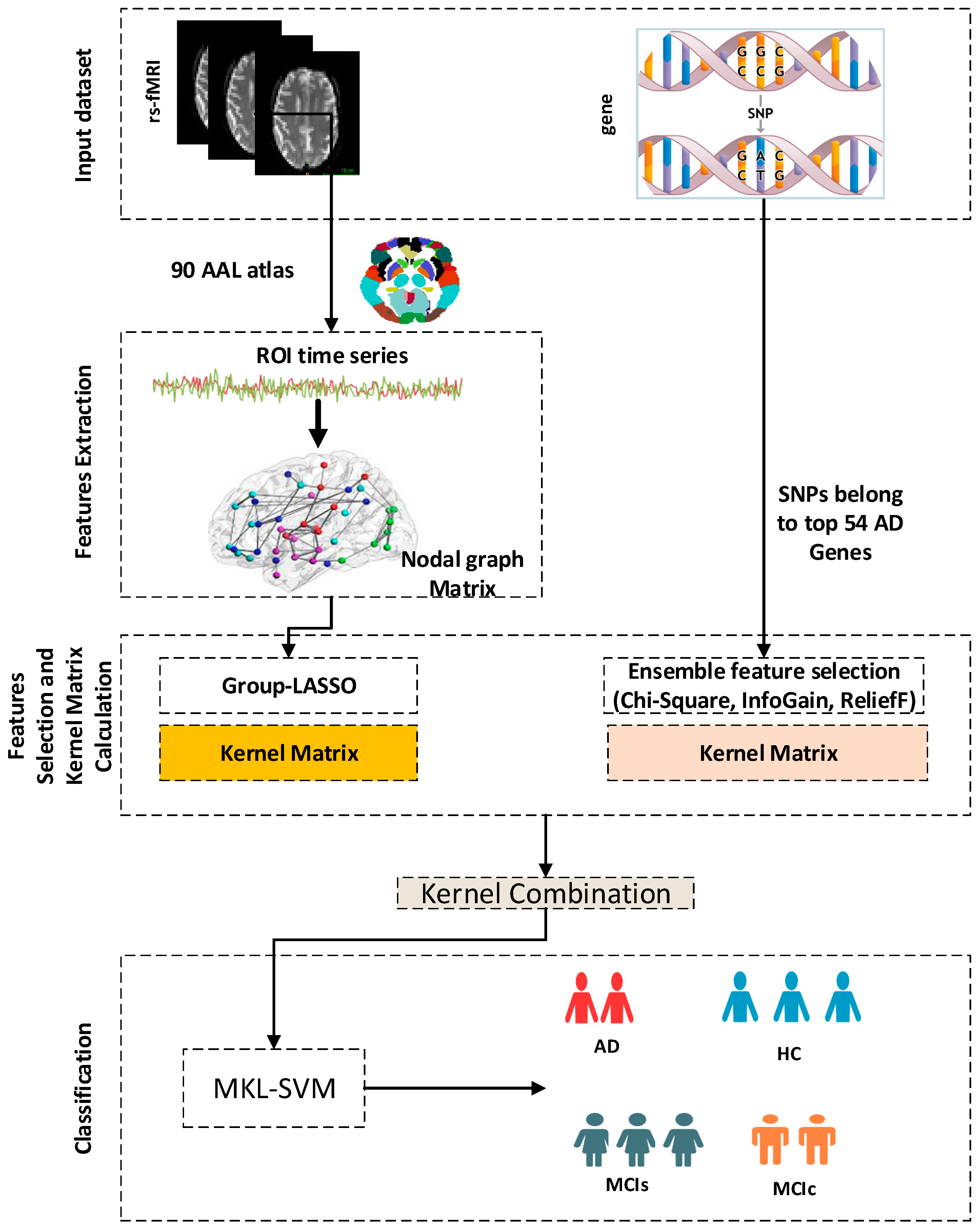
Figure 1. Block diagram of the suggested dementia classification method.
Mathematics 11 01529 g001
Figure 2. SNPs feature importance and their corresponding loci used in this study: (a) force plot representing important gene features and (b) top 20 SNPs. As the SHAP value of an SNP increases, the probability of AD is higher.
Mathematics 11 01529 g002
Figure 3. Highly discriminative brain networks nodal feature for (a) AD vs. HC, (b) HC vs. MCI, (c) AD vs. MCI, and (d): MCIs vs. MCIc.
Mathematics 11 01529 g003
Figure 4. Effect of ensemble features selection on Classification accuracy for Alzheimer’s-associated SNPs genes using MKL-SVM: (a) AD vs. HC, (b) AD vs. MCI, (c) HC vs. MCI, and (d) MCIs vs. MCIc.
Mathematics 11 01529 g004
Figure 5. ROC curve (AUC) for individual features set and combination of SNPs and rs-fMRI nodal networks features matrix using MKL-SVM: (a) AD vs. HC, (b) AD vs. MCI, (c) HC vs. MCI, and (d) MCIs vs. MCIc.
Mathematics 11 01529 g005
Figure 6. Cohen’s kappa score for individual and combined features set for different classification groups using MKL-SVM.
Mathematics 11 01529 g006
Figure 7. A bar chart comparing the performance of various classification groups using MKL-SVM: (a) AD vs. HC, (b) AD vs. MCI, (c) HC vs. MCI, and (d) MCIs vs. MCIc.
Mathematics 11 01529 g007aMathematics 11 01529 g007b
Table 1. Detailed demographic information of the participants.
GroupHCMCIsMCIcAD
Nos. of Subjects32333545
Male/Female17/1518/1720/1523/22
Age74.82 ± 7.1373.50 ± 7.473.35 ± 1275.67 ± 8.71
CDR00.50.5 ± 0.40.7 ± (0.3)
Education17.116.0316.5015.83
MMSE18.30 ± 5.129 ± 1.024.8 ± 3.3129.1 ± 1.7
Table 2. AD-related SNPs with position and id.
Gene Symbolrs-IDPositionGene Symbolrs-IDPosition
ADAMTS4rs4575098161155392ECHDC3rs792072111720308
CR1rs6656401207692049SPI1rs374068847380340
CR1rs2093760207786828CELF1rs1083872547557871
CR1rs4844610207802552MS4A6Ars98339259923508
BIN1rs4663105127891427MS4A2rs793320259936926
BIN1rs6733839127892810MS4A6Ars208154559958380
INPP5Drs10933431233981912PICALMrs86761185776544
INPP5Drs35349669234068476PICALMrs1079283285867875
CLNKrs644845311026028PICALMrs385117985868640
MEF2C-AS1rs19098288223420FERMT2rs1712592453391680
HLA-DRB1rs927105832575406FERMT2rs1712594453400629
CD2APrs947311747431284SLC24A4rs1049863392926952
CD2APrs938156347432637SLC24A4rs1288173592932828
CD2APrs1094836347487762SLC24A4rs1259065492938855
GPR141rs271805837841534ADAM10rs44249559022615
GPR141rs472371137844263KAT8rs5973549331133100
PILRArs185978899971834SCIMPrs1132605315138980
ZCWPW1rs1476679100004446ABI3rs2839486447450775
NYAP1rs12539172100091795ABCA7rs1112788921039323
EPHA1rs10808026143099133ABCA7rs37522461056492
EPHA1-AS1rs7810606143108158ABCA7rs41479291063443
EPHA1-AS1rs11771145143110762PVRL2rs4128951245351516
PTK2Brs2883497027195121CD33rs386544451727962
PTK2Brs7322343127219987CASS4rs602487054997568
CLUrs423667327464929CASS4rs601472454998544
CLUrs933189627467686CASS4rs727458155018260
ECHDC3rs1125723811717397APOErs42935845411941
Table 3. Binary classification performance results for different stages of AD using different classifiers.
GroupFeaturesClassifiersAUCACCSENSPECCohen’s Kappa
AD vs. HCSNPsMKL-SVM89.7375.588.3391.2874.41
RF84.5572.3186.8289.1170.12
XGB87.1374.1787.3190.3273.13
rs-fMRIMKL-SVM91.5184.5194.1788.5481.57
RF86.0483.1290.1992.0382.48
XGB92.3173.9591.5792.4885.01
rs-fMRI + SNPsMKL-SVM95.1393.0394.1694.1787.17
RF87.0888.5386.9389.0583.07
XGB90.4592.7190.9193.7585.01
AD vs.MCISNPsMKL-SVM65.1263.3582.3756.7863.87
RF60.1461.0565.4160.1465.78
XGB62.0563.0367.1463.7165.01
rs-fMRIMKL-SVM75.3772.7184.779.5570.13
RF69.4572.4175.1280.0168.01
XGB73.1472.0378.4578.4769.71
rs-fMRI + SNPsMKL-SVM7677.4385.7590.0184.15
RF74.0175.4590.0488.5683.89
XGB74.9276.0388.0191.8885.03
HC vs. MCISNPsMKL-SVM77.2164.7191.0281.4570.44
RF75.7160.1480.7880.0977.31
XGB77.0263.7288.6780.7878.85
rs-fMRIMKL-SVM80.1175.0385.7890.5580.77
RF75.5371.2383.7885.4778.23
XGB78.1874.1181.9187.9880.07
rs-fMRI + SNPsMKL-SVM82.7984.0192.1387.1783.31
RF76.1780.2890.0390.7880.47
XGB78.581.5592.0794.0181.85
MCIs vs. MCIcSNPsMKL-SVM84.3765.7389.0583.777.75
RF74.2363.6287.7875.4575.48
XGB83.3763.7889.0384.7778.97
rs-fMRIMKL-SVM87.173.0888.5182.3381.05
RF81.5470.9885.3382.7882.77
XGB85.0972.5487.0787.4180.32
rs-fMRI + SNPsMKL-SVM91.0783.7390.3192.3783.09
RF88.4582.4791.0493.0178.75
XGB88.9882.9788.9792.8882.79
Table 4. Performance evaluation of the suggested method against relevant state-of-the-art techniques.
ReferenceMethodsModalityNo of SubjectsGroupACCSENSPE
Dukarat et al. [13]Bayesian-Markov-Blanket+Navie BayesFDG-PAET, AV45-PET, SMRI, APOE122 HC/265 sMCI/177 cMCI/144 ADAD vs. NC86.887.586.1
Brand et al. [49]Task-balanced multi-modal feature selectionsMRI, SNPs201 HC/170 AD/352 MCIAD vs. HC/MCI72.8--
Sheng et al. [5]Fisher score+Multitask feature seletion+SVMsMRI, SNPs25 AD/25 EMCI/25 EMCI/25 HCAD vs. HC9810096
LMCI vs. EMCI808872
LMCI vs. HC868884
EMCI vs. HC828084
Bi et al. [50]Cluster evolutionary random forest (CERF)+SVMfMRI, SNPs37 AD/37 EMCI/35 HCAD vs. HC81--
EMCI vs. HC80--
EMCI vs. NC0.8030.7940.856
our methodEnsemble, group-LASSO, MKL-SVMfMRI, SNPs32 HC/33 MCIs/35 MCIc/45 ADAD vs. HC93.0395.1594.17
AD vs. MCI77.4385.7590.01
HC vs. MCI84.0192.1387.17
MCIs vs. MCIc83.7390.3192.37
Disclaimer/Publisher’s Note: The statements, opinions and data contained in all publications are solely those of the individual author(s) and contributor(s) and not of MDPI and/or the editor(s). MDPI and/or the editor(s) disclaim responsibility for any injury to people or property resulting from any ideas, methods, instructions or products referred to in the content.