
Autonomous Navigation System of Indoor Mobile Robots Using 2D Lidar

Abstract
:1. Introduction
- We embed the proposed algorithm into the ROS system [30] to verify the effectiveness of the algorithm;
- In order to improve the stability and accuracy of the SLAM system, an algorithm called LRBPF-SLAM is proposed. In this algorithm, the odometer data in the distribution function is replaced by the 2D Lidar adjacent moment bit pose difference;
- The GBI-RRT algorithm is proposed, which employs target bias sampling to reduce the negative impact of random sampling on path quality, and then optimizes the initial paths through a path reorganization strategy to eliminate redundant paths;
- Extensive simulations were conducted to evaluate the improved algorithms, and the proposed algorithms were also ported to a mobile robot for real scenario experiments. The results of these experiments demonstrate that the proposed method exhibits excellent performance compared to other algorithms in both simulation and real scenarios.
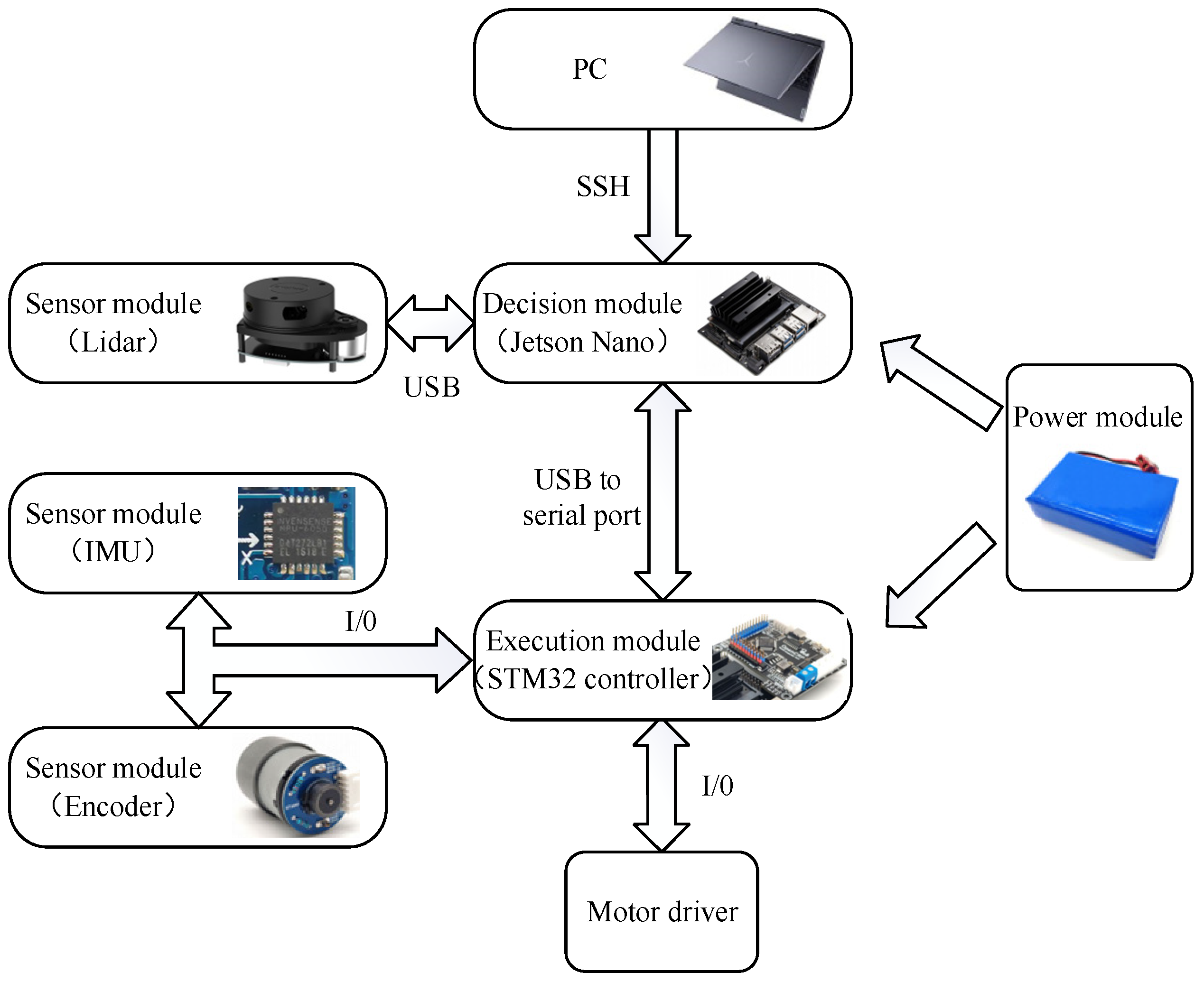
2. Robot Components and System Framework
- The PC Module: The PC terminal uses a laptop and connects to the host computer on the same LAN via SSH (Secure Shell). Commands can be directly sent from the PC to the mobile robot host computer to achieve SLAM and navigation functions;
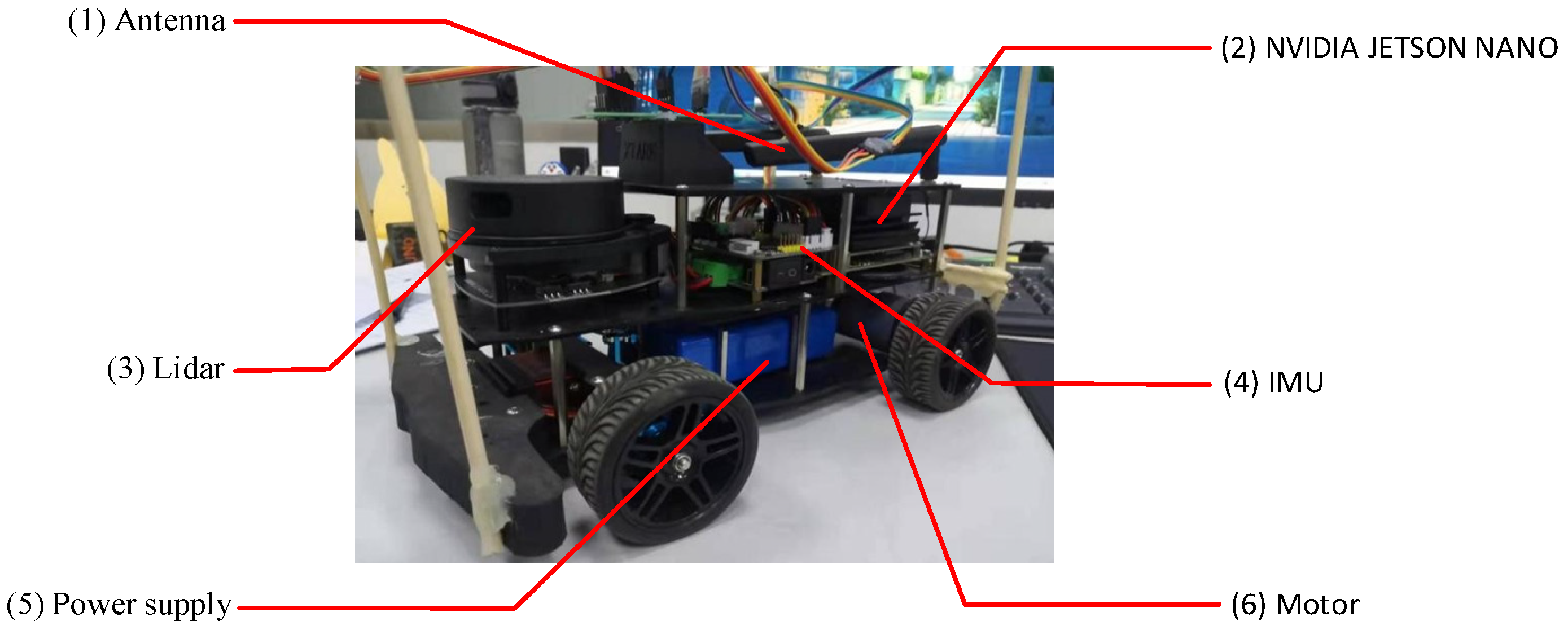
- The Decision Module: The decision module is the host computer of the robot, namely NVIDIA Jetson Nano, which has an SSH tool installed with the ROS system to receive commands from the PC and run algorithms. It receives Lidar data through a USB interface, communicates I/O with the lower computer, and acquires sensor data connected to the lower computer;
- The Execution Module: The execution module is a controller with STM32F4 as its core, which receives commands from the decision-making module, acquires data from the IMU and encoders, and controls motor drive operations;
- The Sensor Module: The sensor module includes 2D Lidar for detecting the surrounding environment, IMU for estimating the motion posture of the robot, and encoders for estimating the robot’s motion distance and rotation angle;
- The Power Module: The power voltage is 12 V with a total capacity of 1200 mAh. The power expansion board can expand the 12 V power and 5 V output to facilitate the expansion of robot functions;
- The Motor Drive Module: The motor drive module is responsible for controlling the movement of the robot, receiving control commands, and driving the motor through current control. It includes the drive circuit, current sensor, and control circuit, ensuring the precise and stable movement of the robot.
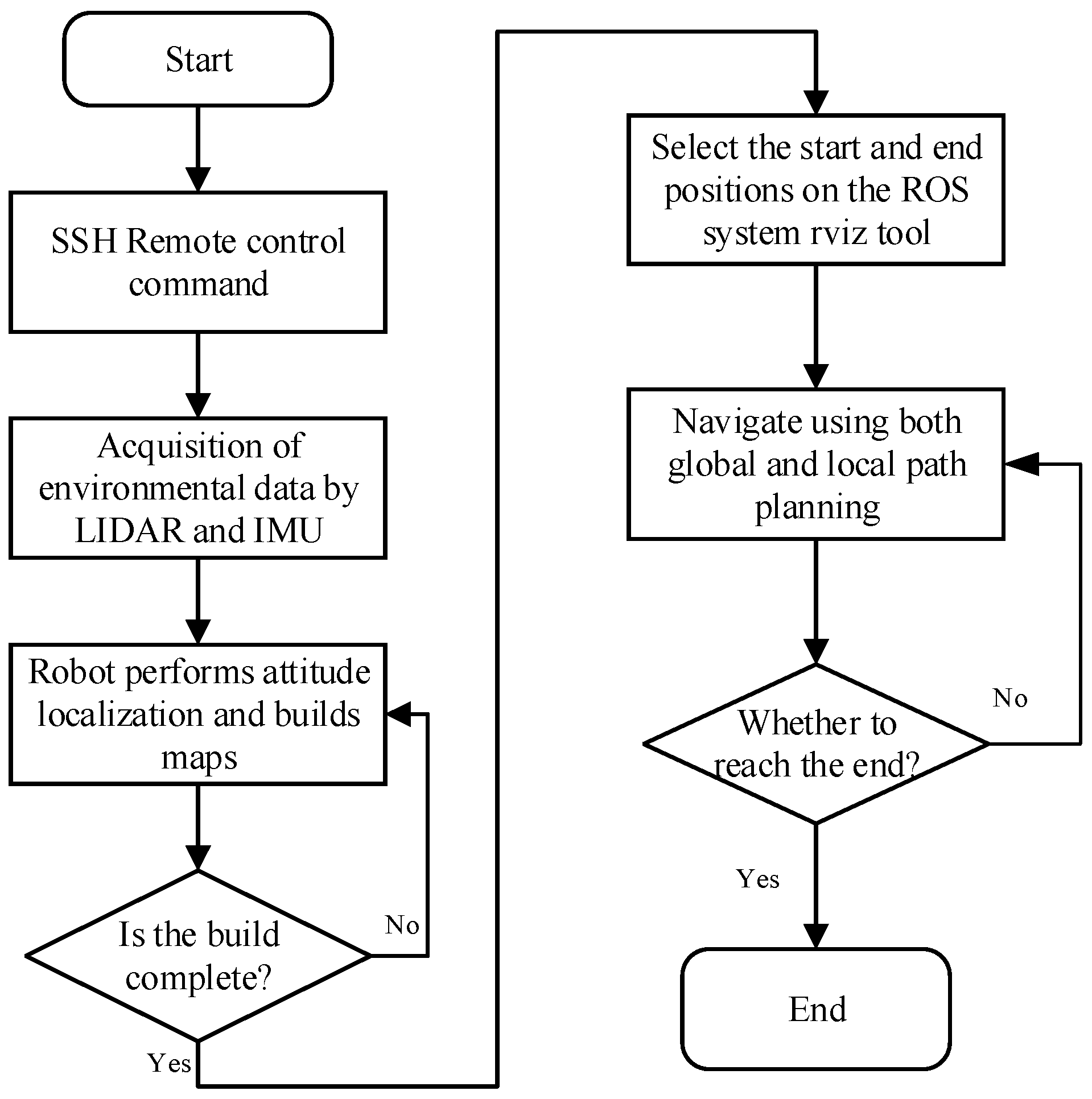
- Install the Ubuntu operating system and ROS system on the robot and PC side, use the SSH remote control tool to realize the connection between the PC and the robot, and control the robot through PC input commands;
- After receiving the PC command, the robot locates and builds a map using the data from the Lidar, and when the mapping is completed, the map is saved in the robot;
- After starting the navigation command, the starting point and the end point are selected on the Rviz (a 3D visualization tool) visualization tool of ROS, and the robot autonomously plans the navigation path using the data from Lidar. The global path planning realizes safe and reliable path planning, and local path planning realizes real-time obstacle avoidance;
- When the robot arrives at the destination, the navigation ends. If it does not reach the destination, it continues to navigate using the data from Lidar until it reaches the destination.
3. Algorithm Improvement
3.1. LRBPF-SLAM Algorithm
- Sampling: The particle at the previous moment is sampled from the distribution function to acquire new particles . The distribution function obtained by the sensor is often termed the proposed distribution:
- Importance weighting: Each particle is assigned a weight , which is computed as the ratio of the posterior distribution to the proposal distribution (based on the probabilistic odometry motion model). The higher the weight, the more the particle’s pose matches the true value. The importance weighting can be defined using Formula (3).
- Resampling: Particles with smaller weights are discarded and replaced by resampled particles, but the total number of particles remains constant.
- Map updating: Each particle’s map is updated using the optimized pose represented by the particle and the current observations.
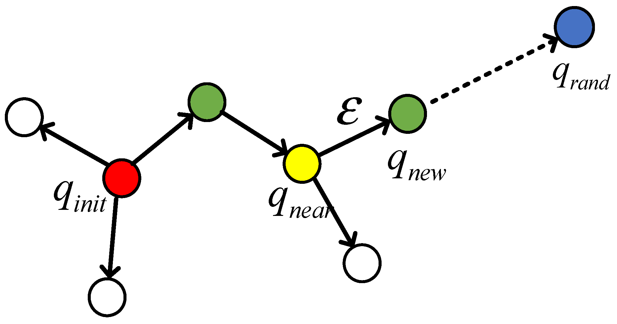
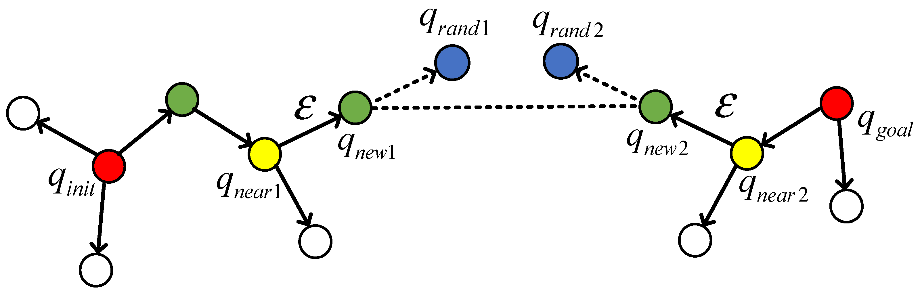
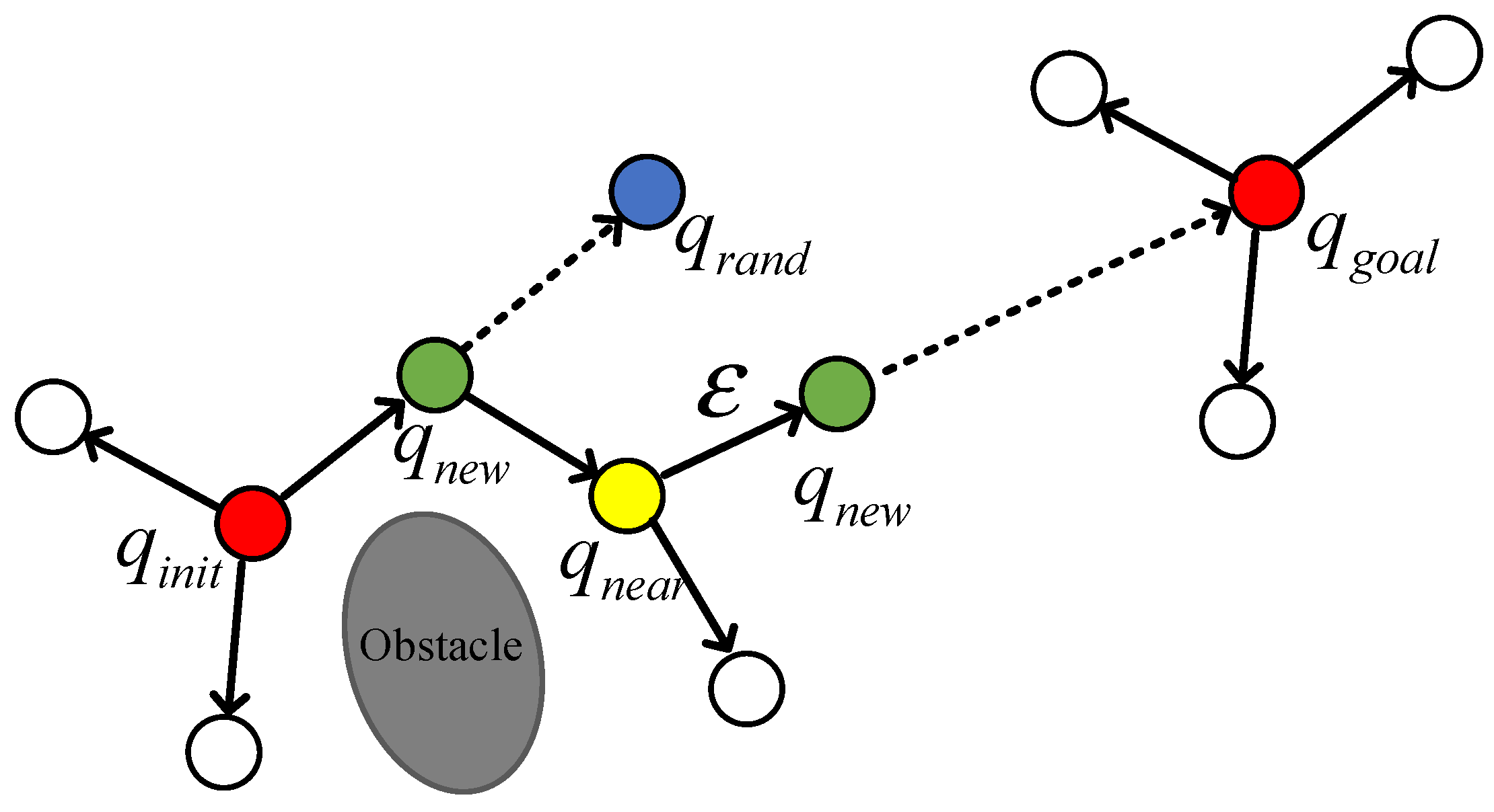
3.2. GBI-RRT Algorithm
| Algorithm 1: |
| 1 |
| 2 |
| 3 |
| 4 |
| 5 |
| 6 |
| 7 |
| 8 |
| 9 |
- Target bias sampling
- 2.
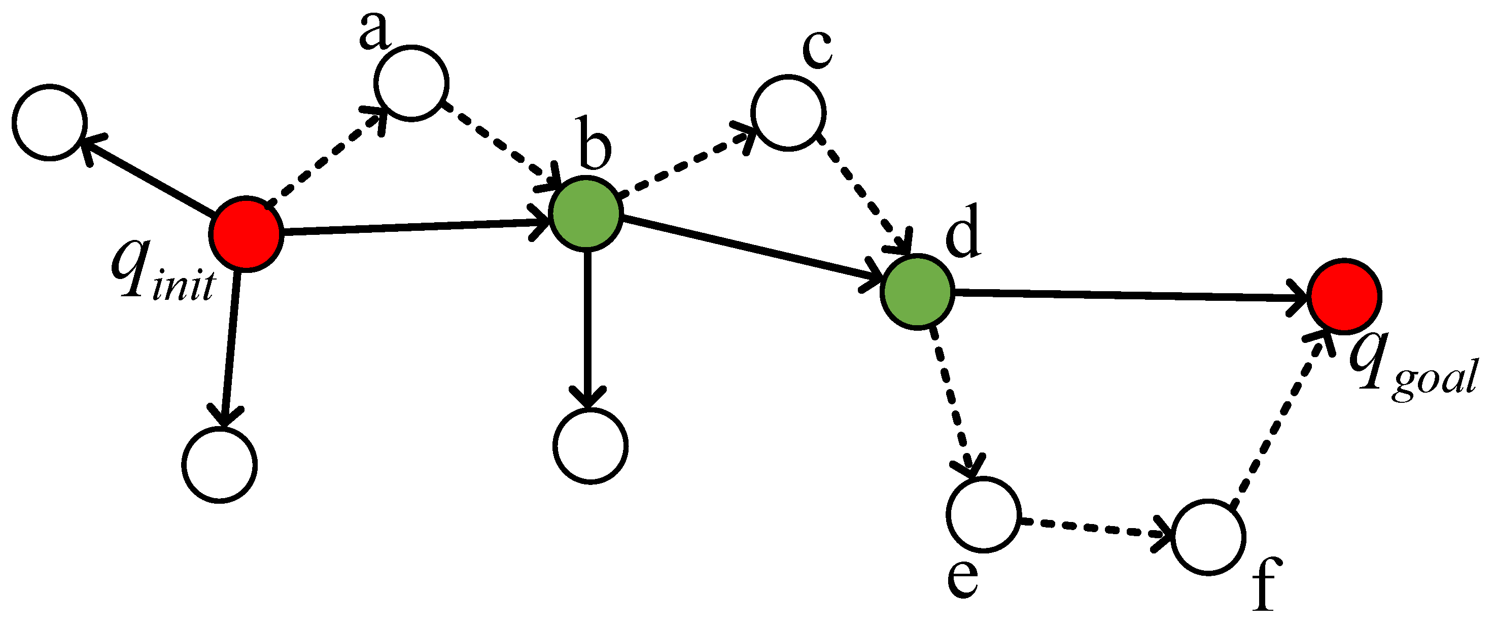
- Path reorganization strategy
| Algorithm 2: |
| 1 |
| 2 |
| 3 |
| 4 |
| 5 |
| 6 |
4. Simulation Experiments of Robots
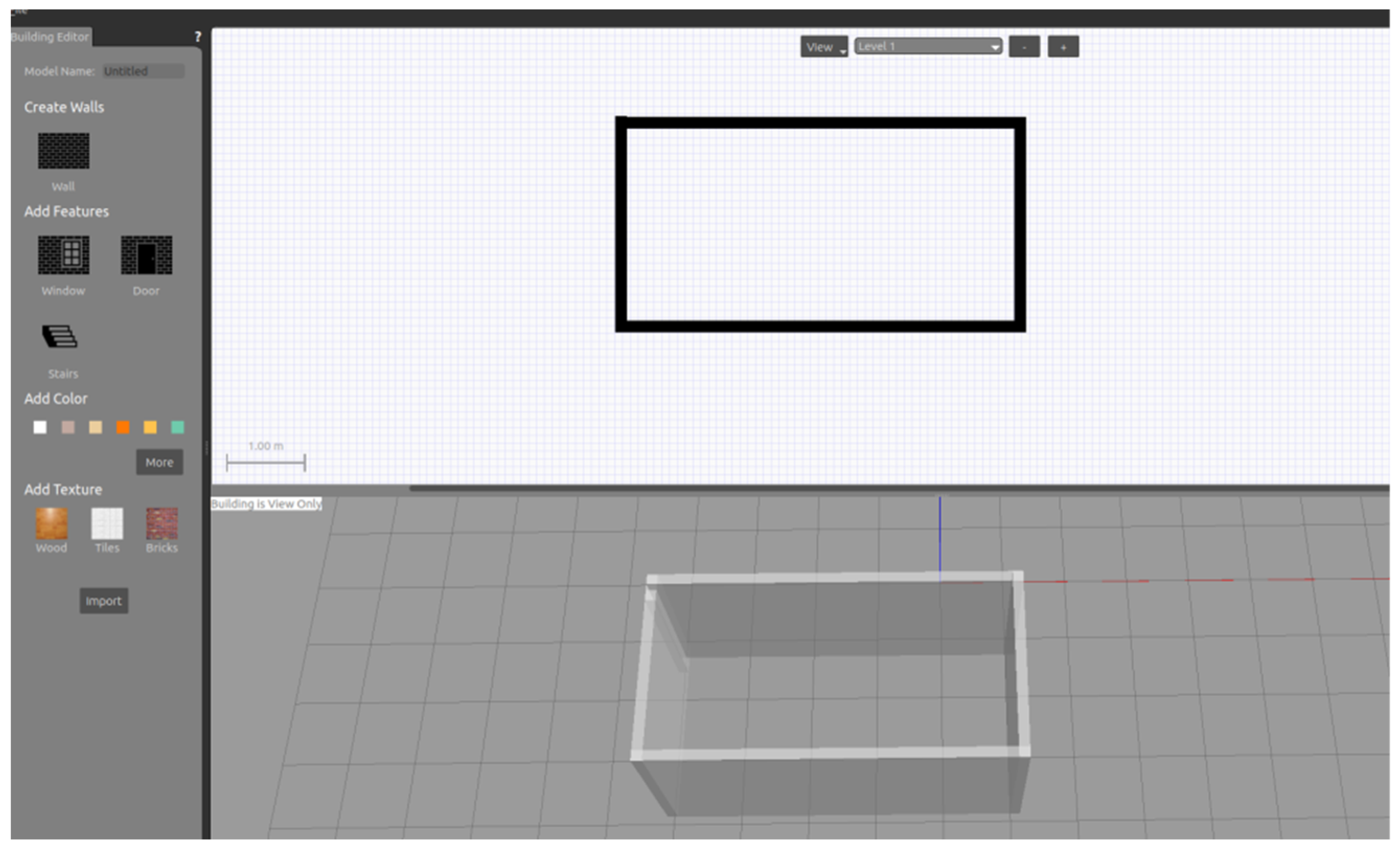
4.1. Simulation Platform
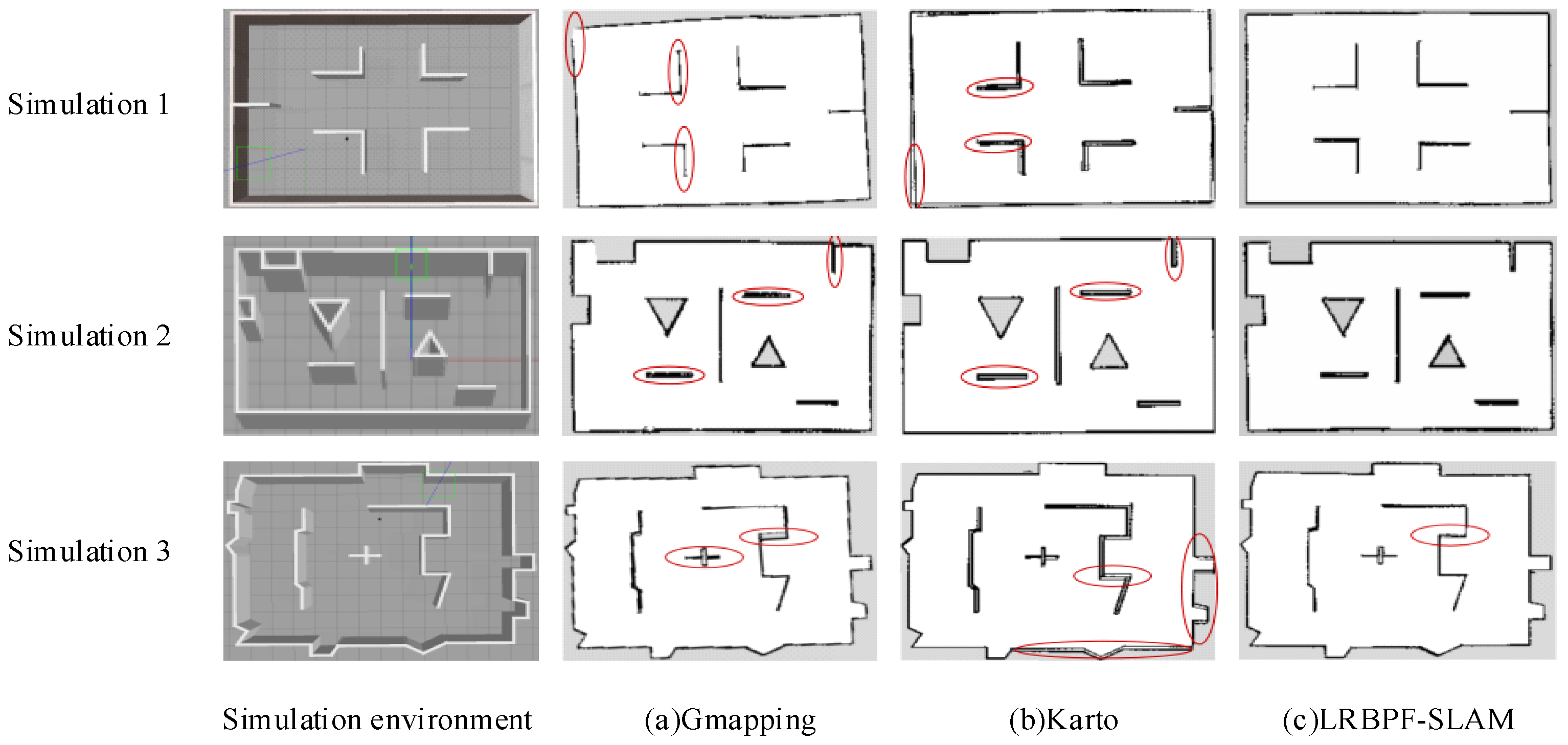
4.2. Simulation Experiment of SLAM Algorithm
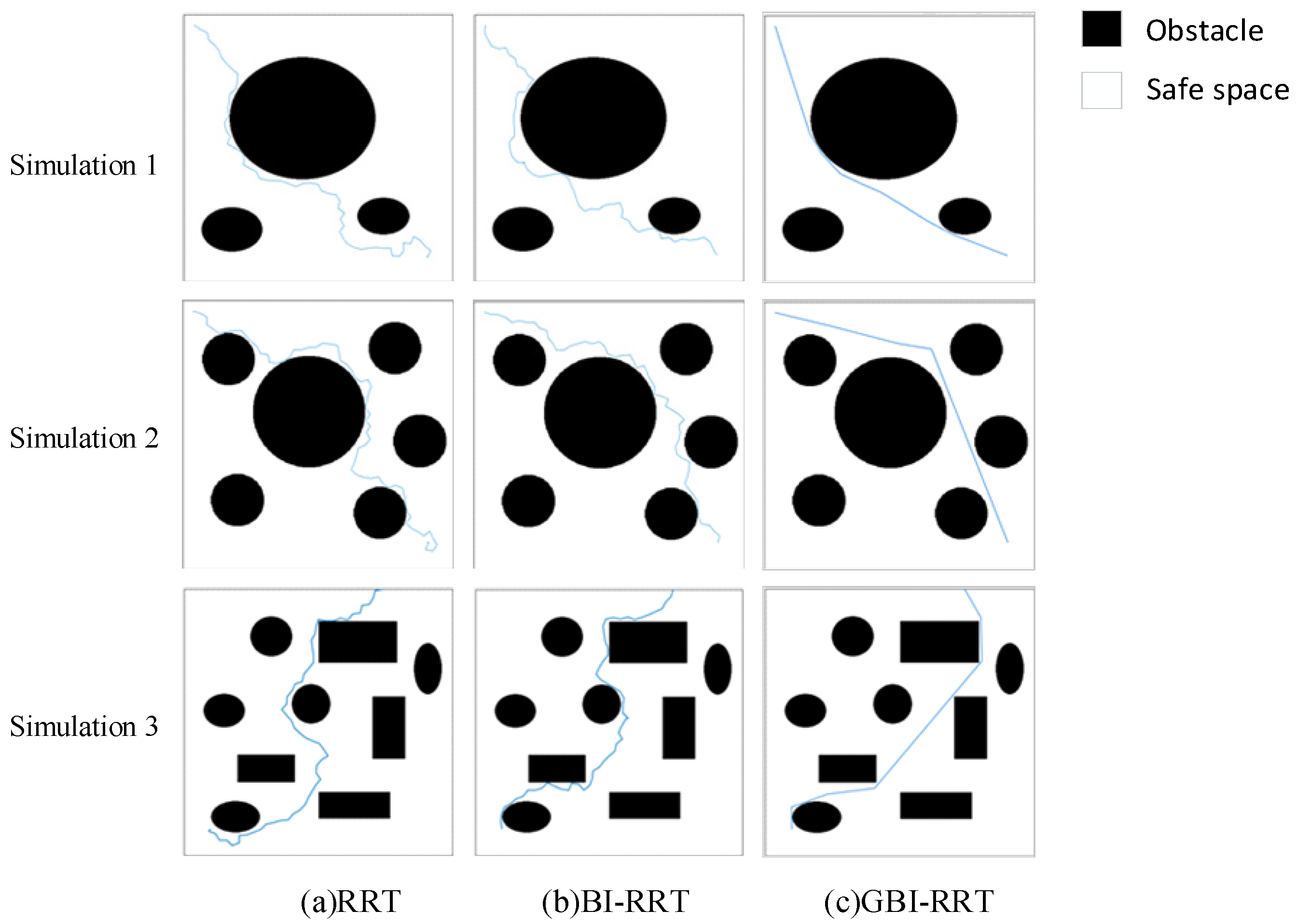
4.3. Simulation Experiment of GBI-RRT Algorithm
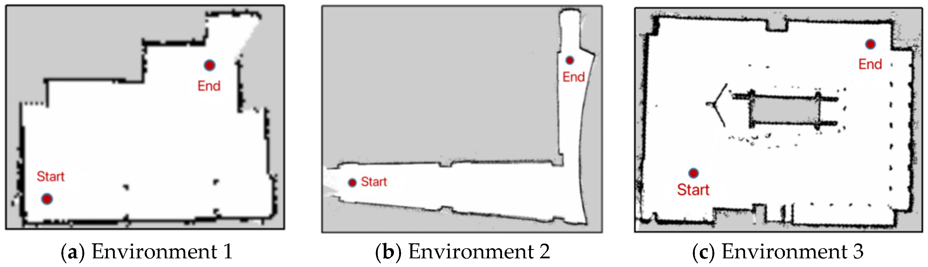
5. Real Scenario Experiments for Robots
5.1. Real Scenario Experiment Setup
- Host controller Jetson Nano and laptop are connected to the same network. A hotspot network on the phone is used to cover the robot’s movement area.
- The “ifconfig” command is used to check the IP addresses of the Jetson Nano and the laptop.
- In the Ubuntu system of the laptop, the environment variables “ROS_MASTER_URI” and “ROS_HOSTNAME_URI” are added to the “bashrc” file. “ROS_MASTER_URI” points to the IP address of the Jetson Nano, while “ROS_HOSTNAME_URI” points to the IP address of the Ubuntu system on the laptop.
- Finally, the robot is remotely accessed using SSH commands in the Ubuntu system terminal for visual remote control. This remote access method makes the robot more visible and makes it easier for the operator to control. These configuration measures greatly improved the efficiency and flexibility of the robot’s tasks.
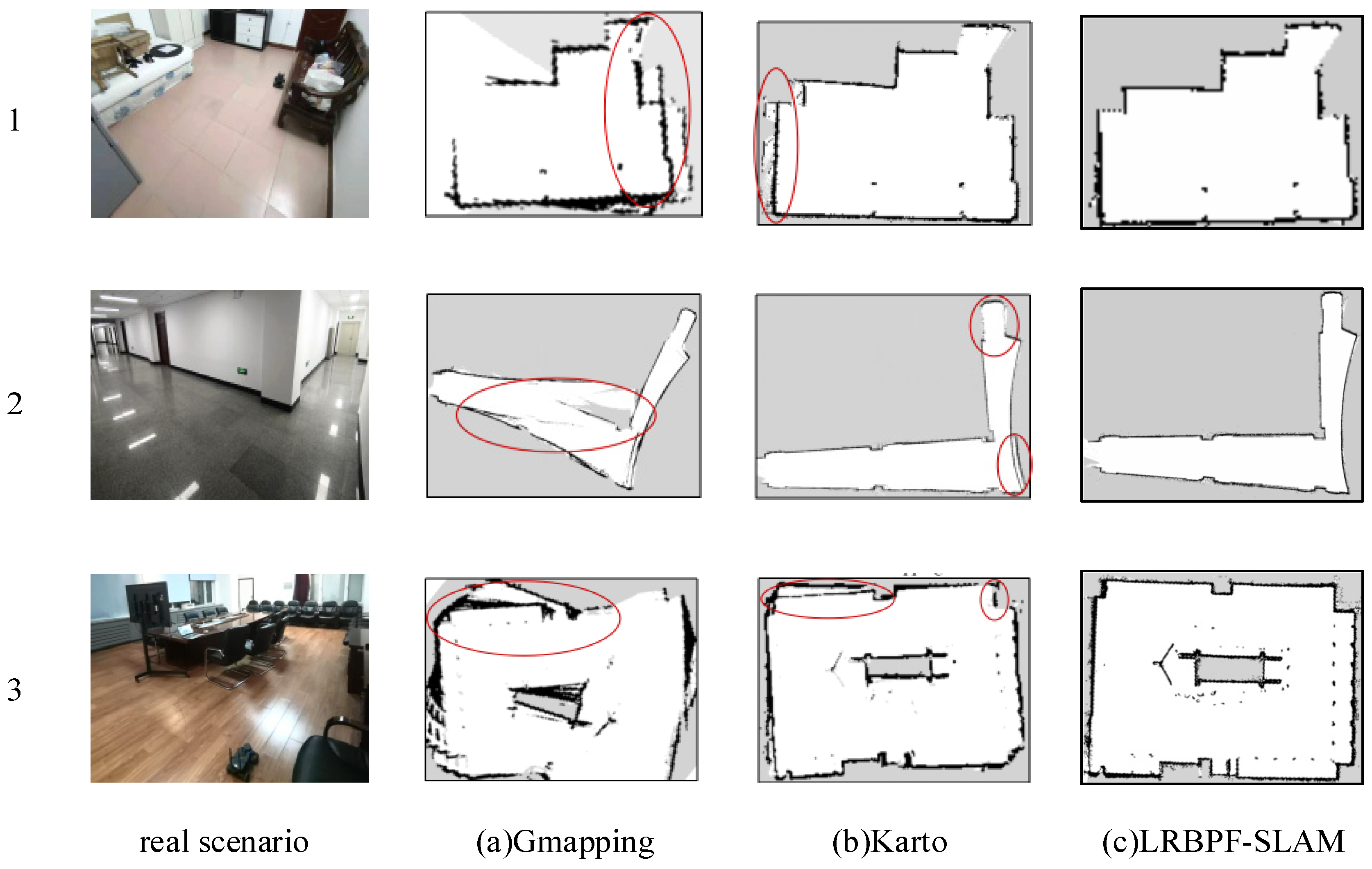
5.2. Experiment of SLAM Algorithm
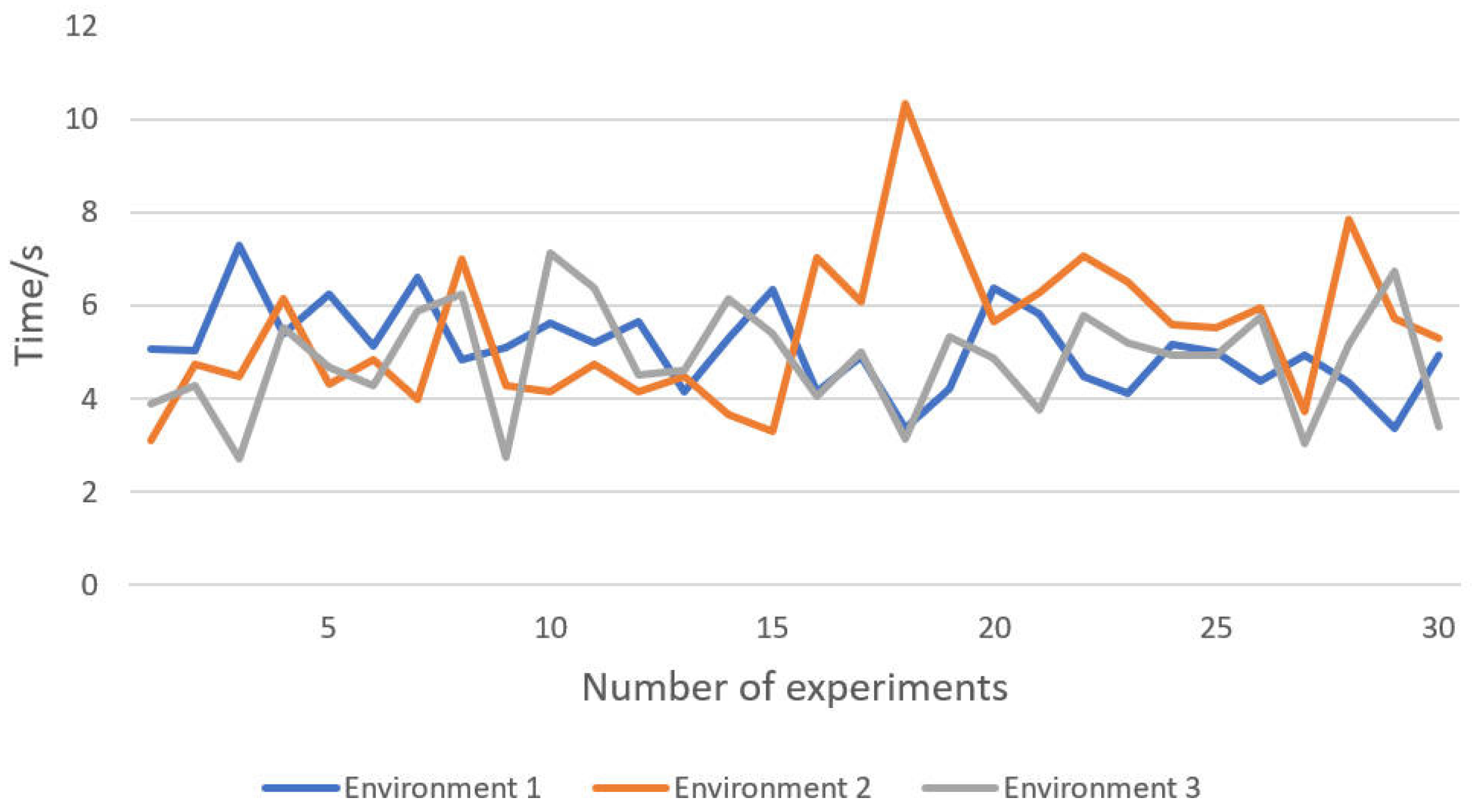
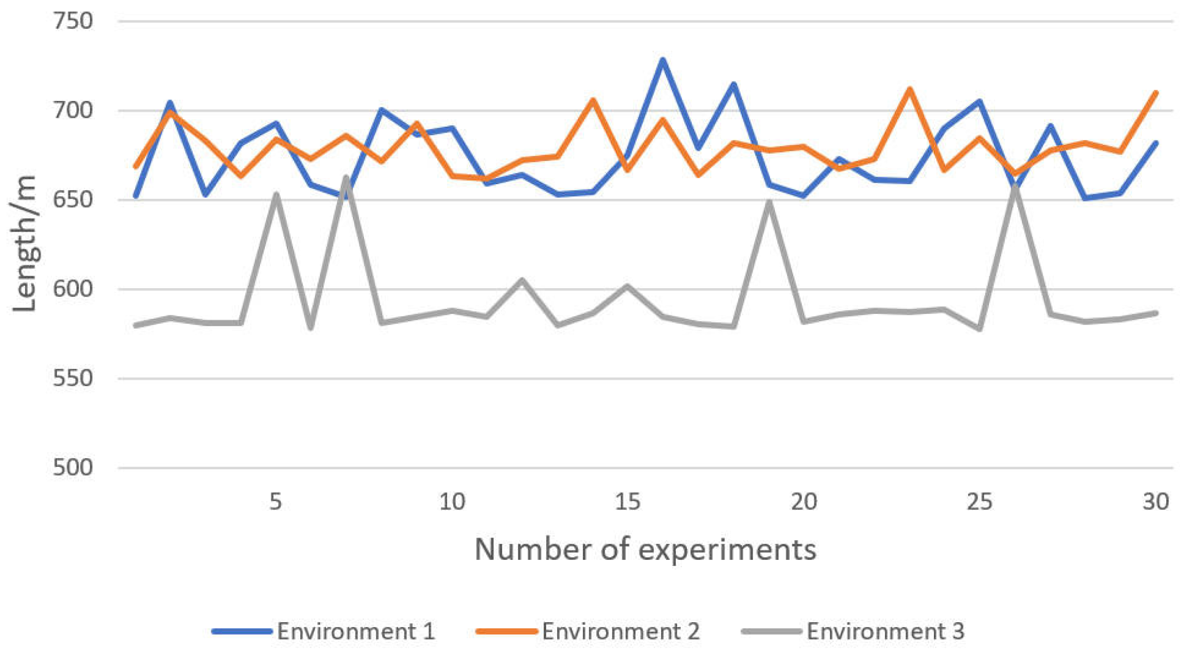
5.3. Experiment of Path Planning Algorithm
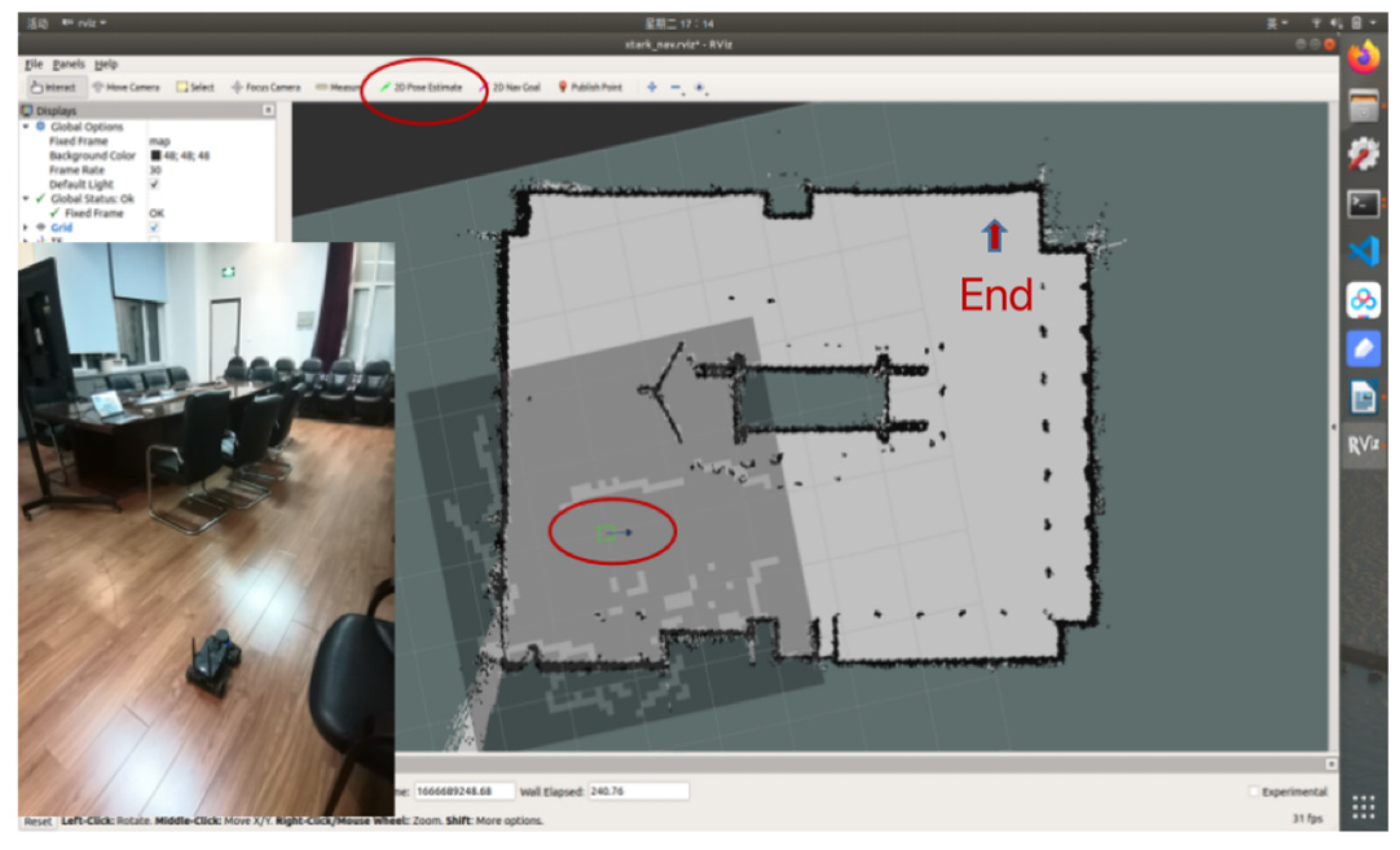
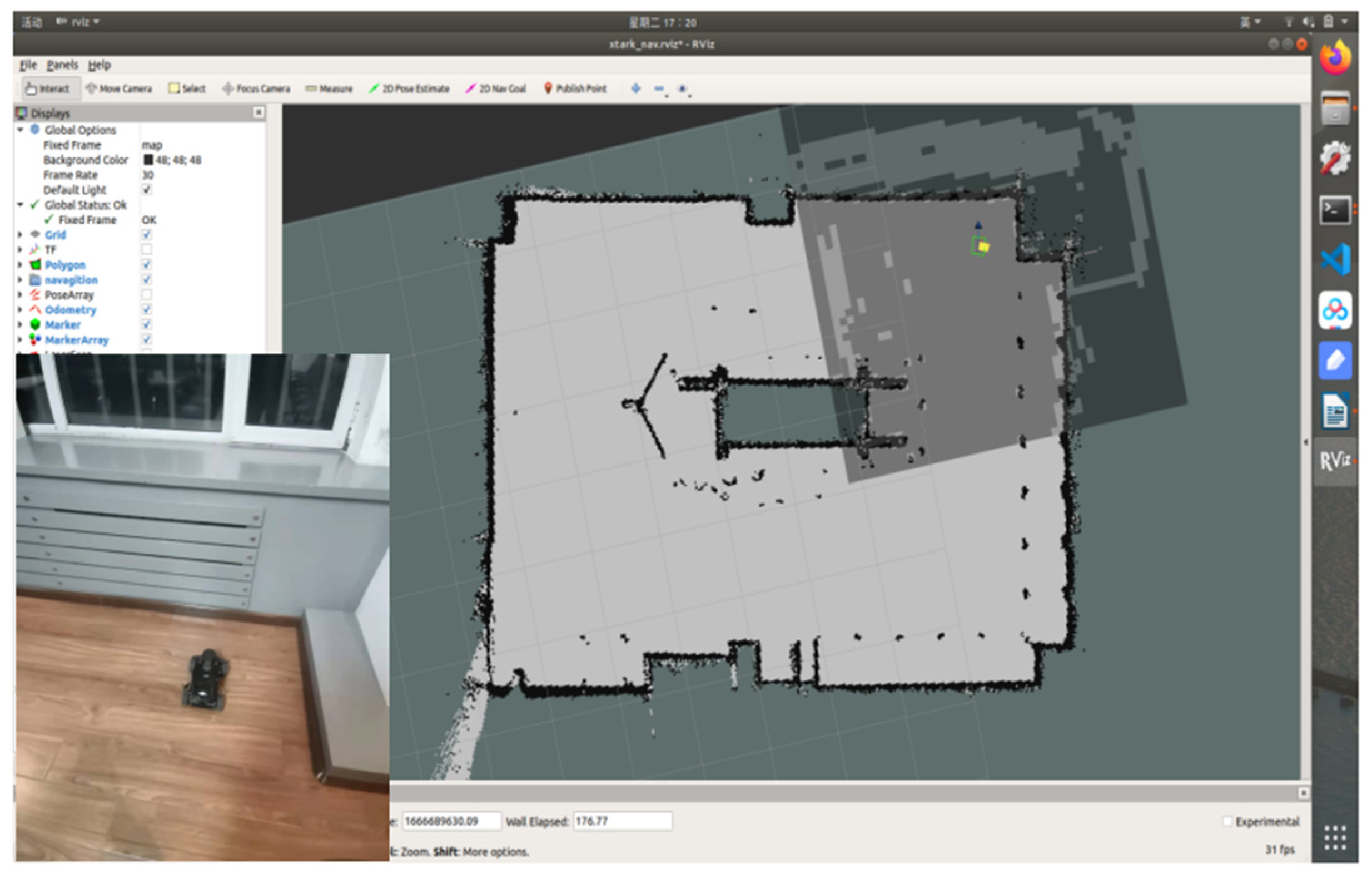
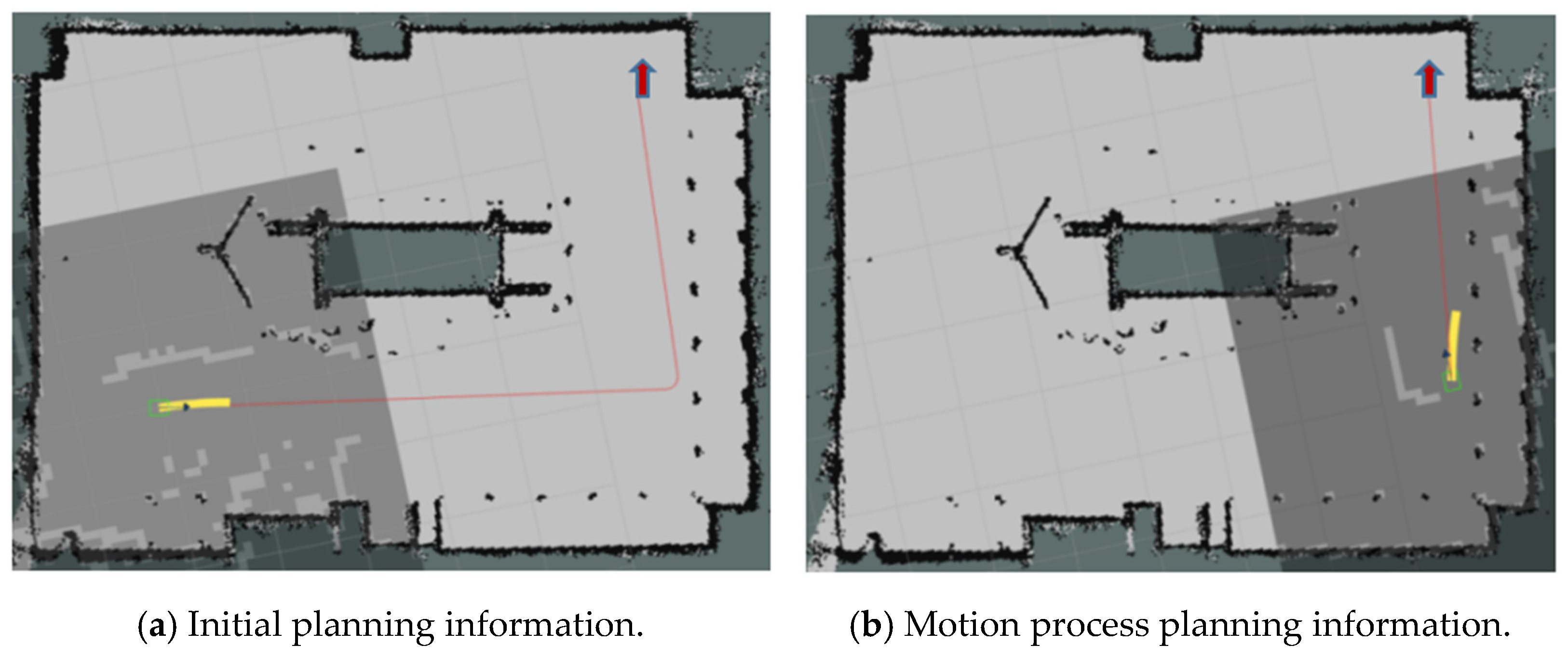
5.4. Robot Navigation Process
6. Conclusions
Author Contributions
Funding
Data Availability Statement
Acknowledgments
Conflicts of Interest
References
- Py, F.; Robbiani, G.; Marafioti, G.; Ozawa, Y.; Watanabe, M.; Takahashi, K.; Tadokoro, S. SMURF software architecture for low power mobile robots: Experience in search and rescue operations. In Proceedings of the 2022 IEEE International Symposium on Safety, Security, and Rescue Robotics (SSRR), Sevilla, Spain, 8–10 November 2022; pp. 264–269. [Google Scholar] [CrossRef]
- Sui, L.; Lin, L. Design of Household Cleaning Robot Based on Low-cost 2D LIDAR SLAM. In Proceedings of the 2020 International Symposium on Autonomous Systems (ISAS), Guangzhou, China, 6–8 December 2020; pp. 223–227. [Google Scholar] [CrossRef]
- Farooq, M.U.; Eizad, A.; Bae, H.-K. Power solutions for autonomous mobile robots: A survey. Robot. Auton. Syst. 2023, 159, 104285. [Google Scholar] [CrossRef]
- Ismail, H.; Roy, R.; Sheu, L.-J.; Chieng, W.-H.; Tang, L.-C. Exploration-Based SLAM (e-SLAM) for the Indoor Mobile Robot Using Lidar. Sensors 2022, 22, 1689. [Google Scholar] [CrossRef]
- Gao, L.; Dong, C.; Liu, X.; Ye, Q.; Zhang, K.; Chen, X. Improved 2D laser slam graph optimization based on Cholesky de-composition. In Proceedings of the 2022 8th International Conference on Control, Decision and Information Technologies (CoDIT), Istanbul, Turkey, 17–20 May 2022; Volume 1, pp. 659–662. [Google Scholar]
- Hampton, B.; Al-Hourani, A.; Ristic, B.; Moran, B. RFS-SLAM robot: An experimental platform for RFS based occupancy-grid SLAM. In Proceedings of the 2017 20th International Conference on Information Fusion (Fusion), Xi’an, China, 10–13 July 2017. [Google Scholar]
- Juric, A.; Kendes, F.; Markovic, I.; Petrovic, I. A Comparison of Graph Optimization Approaches for Pose Estimation in SLAM. In Proceedings of the 2021 44th International Convention on Information, Communication and Electronic Technology (MIPRO), Opatija, Croatia, 27 September–1 October 2021; pp. 1113–1118. [Google Scholar] [CrossRef]
- Dhaoui, R.; Rahmouni, A. Mobile Robot Navigation in Indoor Environments: Comparison of Lidar-Based 2D SLAM Algorithms. In Design Tools and Methods in Industrial Engineering II: Proceedings of the Second International Conference on Design Tools and Methods in Industrial Engineering, ADM 2021, Rome, Italy, 9–10 September 2021; Springer International Publishing: Berlin/Heidelberg, Germany, 2021; pp. 569–580. [Google Scholar]
- Konolige, K.; Grisetti, G.; Kümmerle, R.; Burgard, W.; Limketkai, B.; Vincent, R. Efficient sparse pose adjustment for 2D map-ping. In Proceedings of the 2010 IEEE/RSJ International Conference on Intelligent Robots and Systems, Taipei, Taiwan, 18–22 October 2010; pp. 22–29. [Google Scholar]
- Ribeiro, M.I. Kalman and extended kalman filters: Concept, derivation and properties. Inst. Syst. Robot. 2004, 43, 3736–3741. [Google Scholar]
- Talwar, D.; Jung, S. Particle filter-based Localization of a mobile robot by using a single Lidar sensor under SLAM in ROS environment. In Proceedings of the 2019 19th International Conference on Control, Automation and Systems (ICCAS), Jeju, Republic of Korea, 15–18 October 2019; Volume 43, pp. 3736–3741. [Google Scholar] [CrossRef]
- Cai, Y.; Qin, T. Design of Multisensor Mobile Robot Vision Based on the RBPF-SLAM Algorithm. Math. Probl. Eng. 2022, 2022, 1518968. [Google Scholar] [CrossRef]
- Dai, Y.; Zhao, M. Grey Wolf Resampling-Based Rao-Blackwellized Particle Filter for Mobile Robot Simultaneous Localization and Mapping. J. Robot. 2021, 2021, 4978984. [Google Scholar] [CrossRef]
- Tee, Y.K.; Han, Y.C. Lidar-based 2D SLAM for mobile robot in an indoor environment: A review. In Proceedings of the 2021 International Conference on Green Energy, Computing and Sustainable Technology (GECOST), Miri, Malaysia, 7–9 July 2021; pp. 1–7. [Google Scholar] [CrossRef]
- Maziarz, B.; Domański, P.D. Customized fastSLAM algorithm: Analysis and assessment on real mobile platform. Nonlinear Dyn. 2022, 110, 669–691. [Google Scholar] [CrossRef]
- Muhammad, A.; Ali Mohammed, A.H.; Turaev, S.; Abdulghafor, R.; Shanono, I.H.; Alzaid, Z.; Alruban, A.; Alabdan, R.; Dutta, A.K.; Almotairi, S. A Generalized Laser Simulator Algorithm for Mobile Robot Path Planning with Obstacle Avoidance. Sensors 2022, 22, 8177. [Google Scholar] [CrossRef]
- LaValle, S.M. Rapidly-exploring random trees: A new tool for path planning. Annu. Res. Rep. 1998. [Google Scholar]
- Dijkstra, E.W. A Note on Two Problems in Connexion with Graphs. In Edsger Wybe Dijkstra: His Life, Work, and Legacy; ACM: New York, NY, USA, 2022; pp. 287–290. [Google Scholar] [CrossRef]
- Jin, J.; Zhang, Y.; Zhou, Z.; Jin, M.; Yang, X.; Hu, F. Conflict-based search with D* lite algorithm for robot path planning in unknown dynamic environments. Comput. Electr. Eng. 2023, 105, 108473. [Google Scholar] [CrossRef]
- Liu, B.; Liu, C. Path planning of mobile robots based on improved RRT algorithm. J. Phys. Conf. Ser. 2022, 2216, 012020. [Google Scholar] [CrossRef]
- Pohl, I. BI-Directional and Heuristic Search in Path Problems; Stanford Linear Accelerator Center: Menlo Park, CA, USA, 1969. [Google Scholar]
- Li, Z.; Li, L.; Zhang, W.; Wu, W.; Zhu, Z. Research on Unmanned Ship Path Planning based on RRT Algorithm. J. Phys. Conf. Ser. 2022, 2281, 012004. [Google Scholar] [CrossRef]
- Zhang, X.; Zhu, T.; Du, L.; Hu, Y.; Liu, H. Local Path Planning of Autonomous Vehicle Based on an Improved Heuristic Bi-RRT Algorithm in Dynamic Obstacle Avoidance Environment. Sensors 2022, 22, 7968. [Google Scholar] [CrossRef] [PubMed]
- Xu, J.; Tian, Z.; He, W.; Huang, Y. A fast path planning algorithm fusing PRM and P-BI-RRT. In Proceedings of the 2020 11th International Conference on Prognostics and System Health Management (PHM-2020 Jinan), Jinan, China, 23–25 October; pp. 503–508.
- Gan, Y.; Zhang, B.; Ke, C.; Zhu, X.F.; He, W.M.; Ihara, T. Research on Robot Motion Planning Based on RRT Algorithm with Nonholonomic Constraints. Neural Process. Lett. 2021, 53, 3011–3029. [Google Scholar] [CrossRef]
- Wang, J.; Li, B.; Meng, M.Q.-H. Kinematic Constrained Bi-directional RRT with Efficient Branch Pruning for robot path planning. Expert Syst. Appl. 2020, 170, 114541. [Google Scholar] [CrossRef]
- Grothe, F.; Hartmann, V.N.; Orthey, A.; Toussaint, M. ST-RRT*: Asymptotically-Optimal Bidirectional Motion Planning through Space-Time. arXiv 2022, arXiv:2203.02176. [Google Scholar]
- Zhao, H. Path Planning of Mobile Robots Based on Improved Bi-RRT Algorithm. In Proceedings of the 2022 IEEE 5th International Conference on Automation, Electronics and Electrical Engineering (AUTEEE), Shenyang, China, 18–20 November 2022; pp. 1043–1050. [Google Scholar] [CrossRef]
- Ma, G.; Duan, Y.; Li, M.; Xie, Z.; Zhu, J. A probability smoothing Bi-RRT path planning algorithm for indoor robot. Future Gener. Comput. Syst. 2023, 143, 349–360. [Google Scholar] [CrossRef]
- Choi, J.; Jeong, B.; Theotokatos, G.; Tezdogan, T. Approach an autonomous vessel as a single robot with Robot Operating System in virtual environment. J. Int. Marit. Saf. Environ. Aff. Shipp. 2022, 6, 50–66. [Google Scholar] [CrossRef]
- Kang, J.-G.; Lim, D.-W.; Choi, Y.-S.; Jang, W.-J.; Jung, J.-W. Improved RRT-Connect Algorithm Based on Triangular Inequality for Robot Path Planning. Sensors 2021, 21, 333. [Google Scholar] [CrossRef] [PubMed]
- Zhang, Y.; Wang, H.; Yin, M.; Wang, J.; Hua, C. Bi-AM-RRT*: A Fast and Efficient Sampling-Based Motion Planning Algorithm in Dynamic Environments. arXiv 2023, arXiv:2301.11816. [Google Scholar]
- Platt, J.; Ricks, K. Comparative Analysis of ROS-Unity3D and ROS-Gazebo for Mobile Ground Robot Simulation. J. Intell. Robot. Syst. 2022, 106, 80. [Google Scholar] [CrossRef]
- Li, Y.; Li, J.; Zhou, W.; Yao, Q.; Nie, J.; Qi, X. Robot Path Planning Navigation for Dense Planting Red Jujube Orchards Based on the Joint Improved A* and DWA Algorithms under Laser SLAM. Agriculture 2022, 12, 1445. [Google Scholar] [CrossRef]


| Simulation | Gmapping | Karto | LRBPF-SLAM | |||||
|---|---|---|---|---|---|---|---|---|
| Feature Point | Actual Value/cm | Measured Value/cm | Absolute Error/cm | Measured Value/cm | Absolute Error/cm | Measured Value/cm | Absolute Error/cm | |
| 1 | 1 | 100.00 | 97.99 | 2.01 | 98.48 | 1.52 | 100.86 | 0.86 |
| 2 | 175.00 | 188.15 | 13.15 | 185.60 | 10.60 | 182.33 | 7.33 | |
| 3 Mean | 325.00 - | 341.03 - | 16.03 10.40 | 340.91 - | 15.91 9.34 | 337.50 - | 12.50 6.90 | |
| 2 | 1 | 200.00 | 208.29 | 8.29 | 208.57 | 8.57 | 201.72 | 1.72 |
| 2 | 225.00 | 216.00 | 9.00 | 231.32 | 6.32 | 228.88 | 3.88 | |
| 3 | 200.00 | 196.71 | 3.29 | 204.78 | 4.78 | 197.84 | 2.16 | |
| 4 | 125.00 | 131.14 | 6.14 | 136.52 | 11.52 | 128.02 | 3.02 | |
| 5 Mean | 175.00 - | 169.71 - | 5.29 6.40 | 182.02 - | 7.02 7.64 | 178.45 - | 3.45 2.85 | |
| 3 | 1 | 300.00 | 316.00 | 16.00 | 315.74 | 15.74 | 312.05 | 12.05 |
| 2 | 225.00 | 252.80 | 27.80 | 249.47 | 24.47 | 2370 | 12.00 | |
| 3 | 350.00 | 367.35 | 17.35 | 378.11 | 28.11 | 363.40 | 13.40 | |
| 4 | 300.00 | 316.00 | 16.00 | 319.64 | 19.64 | 308.10 | 8.10 | |
| 5 Mean | 400.00 - | 410.8 - | 10.80 17.59 | 409.29 - | 9.29 19.45 | 410.80 - | 10.80 11.27 | |
| Simulation | Algorithm | Time/s | Length/m |
|---|---|---|---|
| 1 | RRT | 58.79 | 860.24 |
| Bi-RRT | 16.18 | 854.30 | |
| GBI-RRT | 5.08 | 674.45 | |
| 2 | RRT | 98.88 | 880.39 |
| Bi-RRT | 13.19 | 859.37 | |
| GBI-RRT | 5.46 | 679.21 | |
| 3 | RRT | 110.50 | 803.90 |
| Bi-RRT | 5.28 | 777.35 | |
| GBI-RRT | 4.84 | 594.14 |
| Experiment | Gmapping | Karto | LRBPF-SLAM | |||||
|---|---|---|---|---|---|---|---|---|
| Feature Point | Actual Value/cm | Measured Value/cm | Absolute Error/cm | Measured Value/cm | Absolute Error/cm | Measured Value/cm | Absolute Error/cm | |
| 1 | 1 | 42.00 | 45.30 | 3.30 | 45.48 | 3.48 | 46.92 | 4.92 |
| 2 | 41.00 | 47.11 | 6.11 | 50.94 | 9.94 | 46.92 | 4.92 | |
| 3 | 50.00 | 48.92 | 1.08 | 49.12 | 0.88 | 50.55 | 0.55 | |
| 4 Mean | 112.00 - | 108.72 - | 3.28 3.44 | 110.98 - | 1.02 3.83 | 111.89 - | 0.11 2.63 | |
| 2 | 1 | 139.00 | 151.00 | 12.00 | 149.60 | 8.30 | 146.50 | 7.50 |
| 2 | 115.00 | 126.40 | 11.40 | 124.35 | 7.35 | 121.00 | 6.00 | |
| 3 | 84.00 | 92.60 | 5.60 | 93.00 | 3.20 | 89.40 | 2.40 | |
| 4 | 104.00 | 114.80 | 10.80 | 112.90 | 5.70 | 111.20 | 5.10 | |
| 5 | 115.00 | 131.30 | 7.80 | 127.70 | 8.50 | 118.60 | 3.60 | |
| 6 Mean | 57.00 - | 63.10 - | 6.10 8.95 | 60.20 - | 3.20 6.04 | 58.40 - | 1.40 4.33 | |
| 3 | 1 | 57.00 | 64.30 | 5.30 | 53.60 | 3.40 | 59.10 | 2.10 |
| 2 | 41.00 | 47.80 | 6.80 | 45.60 | 7.60 | 42.50 | 1.50 | |
| 3 | 370.00 | 382.90 | 12.90 | 379.80 | 9.80 | 378.70 | 5.20 | |
| 4 | 43.00 | 46.50 | 3.50 | 39.90 | 3.10 | 44.80 | 1.80 | |
| 5 Mean | 39.00 - | 42.20 - | 5.20 6.74 | 43.50 - | 4.50 5.68 | 42.10 - | 3.10 2.74 | |
| Environment | Algorithm | Time/s | Length/m | No. of Turns |
|---|---|---|---|---|
| 1 | RRT | 6.95 | 5.97 | 2.65 |
| Bi-RRT | 6.90 | 5.96 | 2.50 | |
| GBI-RRT | 4.55 | 5.24 | 0.45 | |
| 2 | RRT | 31.25 | 18.14 | 7.55 |
| Bi-RRT | 29.90 | 17.31 | 7.20 | |
| GBI-RRT | 26.15 | 16.42 | 4.75 | |
| 3 | RRT | 17.95 | 11.29 | 4.85 |
| Bi-RRT | 17.70 | 11.05 | 4.70 | |
| GBI-RRT | 14.55 | 8.70 | 2.50 |
Disclaimer/Publisher’s Note: The statements, opinions and data contained in all publications are solely those of the individual author(s) and contributor(s) and not of MDPI and/or the editor(s). MDPI and/or the editor(s) disclaim responsibility for any injury to people or property resulting from any ideas, methods, instructions or products referred to in the content. |
© 2023 by the authors. Licensee MDPI, Basel, Switzerland. This article is an open access article distributed under the terms and conditions of the Creative Commons Attribution (CC BY) license (https://creativecommons.org/licenses/by/4.0/).
Share and Cite
Sun, J.; Zhao, J.; Hu, X.; Gao, H.; Yu, J. Autonomous Navigation System of Indoor Mobile Robots Using 2D Lidar. Mathematics 2023, 11, 1455. https://doi.org/10.3390/math11061455
Sun J, Zhao J, Hu X, Gao H, Yu J. Autonomous Navigation System of Indoor Mobile Robots Using 2D Lidar. Mathematics. 2023; 11(6):1455. https://doi.org/10.3390/math11061455
Chicago/Turabian StyleSun, Jian, Jie Zhao, Xiaoyang Hu, Hongwei Gao, and Jiahui Yu. 2023. "Autonomous Navigation System of Indoor Mobile Robots Using 2D Lidar" Mathematics 11, no. 6: 1455. https://doi.org/10.3390/math11061455
APA StyleSun, J., Zhao, J., Hu, X., Gao, H., & Yu, J. (2023). Autonomous Navigation System of Indoor Mobile Robots Using 2D Lidar. Mathematics, 11(6), 1455. https://doi.org/10.3390/math11061455