Numerical Analysis of a Swelling Poro-Thermoelastic Problem with Second Sound

Abstract

In this paper, we analyze, from the numerical point of view, a swelling porous thermo-elastic problem. The so-called second-sound effect is introduced and modeled by using the simplest Maxwell–Cattaneo law. This problem leads to a coupled system which is written by using the displacements of the fluid and the solid, the temperature and the heat flux. The numerical analysis of this problem is performed applying the classical finite element method with linear elements for the spatial approximation and the backward Euler scheme for the discretization of the time derivatives. Then, we prove the stability of the discrete solutions and we provide an a priori error analysis. Finally, some numerical simulations are performed to demonstrate the accuracy of the approximations, the exponential decay of the discrete energy and the dependence on a coupling parameter.

1. Introduction

It is well known that soil mechanics can be used to describe soil’s swelling properties when the water quantity of the soil varies, because it could change the behavior of the infrastructures or the environment (see, for instance, [1,2,3]). Moreover, it has been accepted that the swelling of materials such as soils, drying of fibers, wood or paper are problems involving porous theory.

This swelling process is produced by some phenomena which arise in the micro scale such as, for instance, the effect of osmotic forces, Brownian motion, hydration forces and electrostatics. Thus, the different layers of the material body are filled by metallic cations which come in contact with water molecules. These solvate the ions between the layers and they lead to the swelling of the whole structure. Due to the need to understand the behavior of the solid matrix, produced by the movement and the resulting interaction with the fluids, the modeling of these swelling materials was based on the mixtures theory for porous elastic solids filled with fluid (see, for instance, [4,5]).

Here, we follow the linear theory for binary mixtures introduced by Ieşan and Quintanilla [6]. It was extended later by Quintanilla [7] to include, in the one-dimensional setting, the fluid saturation. He derived it from the one written in the three-dimensional space and proposed by Eringen [8]. From these pioneering works, the number of references dealing with swelling porous problems is huge (see, e.g., [9,10,11,12,13,14,15,16,17,18,19,20,21,22,23,24]), where different analytical (existence and uniqueness, energy decay) and numerical (stability or accuracy) issues are considered.

In this paper, we continue the research started in [25], where the well-posedness and exponential decay of a one-dimensional swelling porous thermoelastic problem was considered. The so-called second-sound effect was also included in the model. These analytical results were proved by using the well-known Lumer–Phillips theorem to establish the well-posedness result of the system described in the next sections, and the multiplier method to show that the system decays in an exponential way for any stability number or without the assumption of similar wave propagation. Therefore, our aim will be to introduce a fully discrete approximation of the resulting variational formulation, by using the finite element method and the implicit Euler scheme. Then, we will prove a discrete stability property and some a priori error estimates and, finally, we will show some numerical results.

The plan of this paper is the following. In Section 2, we present the following problem [25]: we recall an existence and uniqueness result and we derive the variational formulation. Then, a fully discrete scheme is introduced in Section 3, by using the classical finite element method and the implicit Euler scheme, and we provide its numerical analysis. Finally, we show some numerical experiments in Section 4 to demonstrate the efficiency of the approximations, the exponential decay of the discrete energy and the behavior of the solution.

2. Thermomechanical Model

In this section, we follow the recently published paper [25] and we present the mathematical model and we derive its variational formulation.

Let u and z be the displacement of the solid and the fluid, respectively, $\theta$ the temperature and q the heat flux. Since we are working with the simplest Maxwell–Cattaneo law, the following constitutive equation is used:

$$\tau q_t+\beta q+{\theta }_x=0,$$

where $\tau >0$ is called the relaxation time, $\beta >0$ is a constitutive coefficient and subscripts x and t are used to denote the usual derivatives with respect to the spatial and time variables, respectively.

According to [25], the following system of equations must be solved in a given domain $(0,\ell )$, $\ell >0$, over a finite time interval $[0,T]$, $T>0$ being the final time:

$$\left.\begin{array}{c}{\rho }_z{z}_{tt}-{\alpha }_1{z}_{xx}-{\alpha }_2{u}_{xx}=0,\hfill \\ {\rho }_u{u}_{tt}-{\alpha }_3{u}_{xx}-{\alpha }_2{z}_{xx}+\gamma {\theta }_x=0,\hfill \\ {\rho }_{\theta }{\theta }_t+q_x+\gamma u_{xt}=0,\hfill \\ \tau q_t+\beta q+{\theta }_x=0\hfill \end{array}\right\}\mathrm{in}(0,\ell )\times (0,T).$$

(1)

This system of equations must be complemented with some initial and boundary conditions. Therefore, we impose, for a.e. $x\in (0,\ell )$,

$$\begin{array}{c}z(x,0)=z_0\left(x\right),z_t(x,0)=y_0\left(x\right),\theta (x,0)={\theta }_0\left(x\right),\hfill \\ u(x,0)=u_0\left(x\right),u_t(x,0)=v_0\left(x\right),q(x,0)=q_0\left(x\right),\hfill \end{array}$$

(2)

and, for a.e. $t\in (0,T),$

$$z(0,t)=z(\ell ,t)=u(0,t)=u(\ell ,t)=\theta (0,t)=\theta (\ell ,t)=0.$$

(3)

We have used homogeneous Dirichlet boundary conditions in (3) for the sake of simplicity, but it is straightforward to extend the analysis presented in the next section to other physical situations.

In the rest of the paper, we will assume that the densities ${\rho }_u>0$, ${\rho }_z>0$ and ${\rho }_{\theta }>0$ are equal to 1 to simplify the writing.

In [25] the following theorem was proved.

Theorem 1. 

Under the following conditions on the constitutive parameters:

$${\alpha }_1>0,{\alpha }_2\ne 0,{\alpha }_1{\alpha }_3>{\alpha }_2^2,\gamma \ne 0,$$

(4)

if the initial conditions have the regularity:

$$u_0,z_0\in H^1(0,\ell ),v_0,y_0\in L^2(0,\ell ),{\theta }_0,q_0\in H^1(0,\ell ),$$

(5)

then problems (1), (2) and (3) admit a unique solution with the following regularity:

$$\begin{array}{c}u,z\in C^1([0,T];H^1(0,\ell ))\cap C^2([0,T];L^2(0,\ell )),\hfill \\ \theta ,q\in C([0,T];H^1(0,\ell ))\cap C^1([0,T];L^2(0,\ell )).\hfill \end{array}$$

Now, we will obtain the variational formulation of the above swelling porous thermoelastic problem with second sound. Let us denote the variational spaces $H=L^2(0,\ell )$, $E=H^1(0,\ell )$ and $V=H_0^1(0,\ell )$, and let $(·,·)$ and $\parallel ·\parallel$ be the classical inner product and its corresponding norm in $L^2(0,\ell )$, respectively.

If we denote $y=z_t$ and $v=u_t$, integrating by parts the constitutive system (1) and using initial and boundary conditions (2) and (3), we obtain the following weak form of problem (1)–(3):

Find the velocity of the fluid $y:[0,T]\to V$, the velocity of the solid $v:[0,T]\to V$, the temperature $\theta :[0,T]\to V$ and the heat flux $q:[0,T]\to E$ such that $y\left(0\right)=y_0$, $v\left(0\right)=v_0$, $\theta \left(0\right)={\theta }_0$, $q\left(0\right)=q_0$ and, for a.e. $t\in (0,T)$ and for all $w,r,s\in V$ and $m\in E$,

$$\begin{array}{ccc}& & {\displaystyle (y_t\left(t\right),w)+{\alpha }_1(z_x\left(t\right),w_x)+{\alpha }_2(u_x\left(t\right),w_x)=0,}\hfill \end{array}$$

(6)

$$\begin{array}{ccc}& & {\displaystyle (v_t\left(t\right),r)+{\alpha }_3(u_x\left(t\right),r_x)+{\alpha }_2(z_x\left(t\right),r_x)+\gamma ({\theta }_x\left(t\right),r)=0,}\hfill \end{array}$$

(7)

$$\begin{array}{ccc}& & {\displaystyle ({\theta }_t\left(t\right),s)+(q_x\left(t\right),s)+\gamma (v_x\left(t\right),s)=0,}\hfill \end{array}$$

(8)

$$\begin{array}{ccc}& & {\displaystyle \tau (q_t\left(t\right),m)+\beta (q\left(t\right),m)+({\theta }_x\left(t\right),m)=0,}\hfill \end{array}$$

(9)

where the displacements of the fluid and the solid are then found from

$${\displaystyle z\left(t\right)={\int }_0^{t}y\left(s\right)ds+z_0,u\left(t\right)={\int }_0^{t}v\left(s\right)ds+u_0.}$$

(10)

3. Numerical Analysis: A Priori Error Estimates

In this section, we will show a discrete stability property and we will provide an a priori error analysis for a fully discrete approximation of the variational problem (6)–(10).

Therefore, for the spatial approximation of the problem, let us assume that the interval $[0,\ell ]$ is split into M subintervals $a_0=0<a_1<\dots <a_M=\ell$ with the same length $h=a_{i+1}-a_i=\ell /M$. So, let us define the finite element spaces:

$$E^h=\{w^h\in C\left([0,\ell ]\right);w_{[a_i,a_{i+1}]}^h\in P_1\left([a_i,a_{i+1}]\right)i=0,\dots ,M-1\},$$

(11)

and $V^h=E^h\cap V$. Here, $P_1\left([a_i,a_{i+1}]\right)$ represents the space of polynomials of degree less than or equal to one for each subinterval $[a_i,a_{i+1}]$; that is, the finite element spaces $E^h$ and $V^h$ are made by continuous and piecewise linear functions. Moreover, let us construct the discrete initial conditions $z_0^h$, $y_0^h$, $u_0^h$, $v_0^h$, ${\theta }_0^h$ and $q_0^h$ in the following form:

$$\begin{array}{c}{z}_0^h={\mathcal{P}}_1^h{z}_0,y_0^h={\mathcal{P}}_1^h{y}_0,u_0^h={\mathcal{P}}_1^h{u}_0,v_0^h={\mathcal{P}}_1^h{v}_0,\hfill \\ {\theta }_0^h={\mathcal{P}}_1^h{\theta }_0,q_0^h={\mathcal{P}}_2^h{q}_0,\hfill \end{array}$$

(12)

where the operators ${\mathcal{P}}_1^h$ and ${\mathcal{P}}_2^h$ represent the respective finite element interpolation ones over $V^h$ and $E^h$ [26].

Secondly, to discretize the first-order time derivatives, we use a uniform partition of the time interval $[0,T]$, denoted by $0=t_0<t_1<\dots <t_N=T$, with a step size $k=T/N$ and nodes $t_n=nk$ for $n=0,1,\dots ,N$. Moreover, as a usual notation, let $w_n=w\left(t_n\right)$ for a continuous function w and, given a sequence ${\left\{w_n\right\}}_{n=0}^N$, we denote by $\delta w_n=(w_n-w_{n-1})/k$ its divided differences.

By using the well-known implicit Euler scheme for the discretization of the time derivatives, we obtain the following fully discrete scheme which approximates problems (6)–(10).

Find the discrete velocity of the fluid $y^{hk}={\left\{y_n^{hk}\right\}}_{n=0}^N\subset V^h$, the discrete velocity of the solid $v^{hk}={\left\{v_n^{hk}\right\}}_{n=0}^N\subset V^h$, the discrete temperature ${\theta }^{hk}={\left\{{\theta }_n^{hk}\right\}}_{n=0}^N\subset V^h$ and the discrete heat flux $q^{hk}={\left\{q_n^{hk}\right\}}_{n=0}^N\subset E^h$ such that $y_0^{hk}=y_0^h$, $v_0^{hk}=v_0^h$, ${\theta }_0^{hk}={\theta }_0^h$, $q_0^{hk}=q_0^h$ and, for all $w^h,r^h,s^h\in V^h$ and $m^h\in E^h$ and $n=1,\dots ,N$,

$$\begin{array}{ccc}& & {\displaystyle (\delta y_n^{hk},w^h)+{\alpha }_1({\left(z_n^{hk}\right)}_x,w_x^h)+{\alpha }_2({\left(u_n^{hk}\right)}_x,w_x^h)=0,}\hfill \end{array}$$

(13)

$$\begin{array}{ccc}& & {\displaystyle (\delta v_n^{hk},r^h)+{\alpha }_3({\left(u_n^{hk}\right)}_x,r_x^h)+{\alpha }_2({\left(z_n^{hk}\right)}_x,r_x^h)+\gamma ({\left({\theta }_n^{hk}\right)}_x,r^h)=0,}\hfill \end{array}$$

(14)

$$\begin{array}{ccc}& & {\displaystyle (\delta {\theta }_n^{hk},s^h)+({\left(q_n^{hk}\right)}_x,s^h)+\gamma ({\left(v_n^{hk}\right)}_x,s^h)=0,}\hfill \end{array}$$

(15)

$$\begin{array}{ccc}& & {\displaystyle \tau (\delta q_n^{hk},m^h)+\beta (q_n^{hk},m^h)+({\left({\theta }_n^{hk}\right)}_x,m^h)=0,}\hfill \end{array}$$

(16)

where the discrete displacements of the fluid and solid, $z_n^{hk}$ and $u_n^{hk}$, respectively, are obtained as follows:

$${\displaystyle z_n^{hk}=k\sum _{j=1}^n{y}_j^{hk}+z_0^h,u_n^{hk}=k\sum _{j=1}^n{v}_j^{hk}+u_0^h.}$$

(17)

Taking into account assumptions (4) and applying the Lax Milgram lemma, we can immediately show that problem (13)–(17) has a unique discrete solution.

Now, we will numerically analyze the above discrete problem. First, we will show a discrete stability property that we state as follows.

Lemma 1. 

Under the assumptions of Theorem 1, the solution to discrete problem (13)–(17) satisfies the following discrete stability property:

$$\begin{array}{c}\parallel y_n^{hk}{\parallel }^2+\parallel z_n^{hk}{\parallel }_V^2+\parallel v_n^{hk}{\parallel }^2+\parallel u_n^{hk}{\parallel }_V^2+\parallel {\theta }_n^{hk}{\parallel }^2+{\parallel q_n^{hk}\parallel }^2\le C,\hfill \end{array}$$

where ${\parallel ·\parallel }_V$ denotes the usual norm in V, and $C>0$ represents a positive constant which does not depend on parameters h and k.

Proof. 

First, taking $w^h=y_n^{hk}$ is (13) we find that

$$(\delta y_n^{hk},y_n^{hk})+{\alpha }_1({\left(z_n^{hk}\right)}_x,{\left(y_n^{hk}\right)}_x)+{\alpha }_2({\left(u_n^{hk}\right)}_x,{\left(y_n^{hk}\right)}_x)=0,$$

and taking into account that

$$\begin{array}{c}{\displaystyle (\delta y_n^{hk},y_n^{hk})\ge \frac{1}{2k}\left\{\parallel y_n^{hk}{\parallel }^2-{\parallel y_{n-1}^{hk}\parallel }^2\right\},}\hfill \\ {\displaystyle {\alpha }_1({\left(z_n^{hk}\right)}_x,{\left(y_n^{hk}\right)}_x)=\frac{{\alpha }_1}{2k}\left\{\parallel {\left(z_n^{hk}\right)}_x{\parallel }^2-\parallel {\left(z_{n-1}^{hk}\right)}_x{\parallel }^2+\parallel {(z_n^{hk}-z_{n-1}^{hk})}_x{\parallel }^2\parallel \right\},}\hfill \end{array}$$

it follows that

$$\begin{array}{c}{\displaystyle \frac{1}{2k}\left\{\parallel y_n^{hk}{\parallel }^2-{\parallel y_{n-1}^{hk}\parallel }^2\right\}+\frac{{\alpha }_1}{2k}\left\{\parallel {\left(z_n^{hk}\right)}_x{\parallel }^2-\parallel {\left(z_{n-1}^{hk}\right)}_x{\parallel }^2+{\parallel {(z_n^{hk}-z_{n-1}^{hk})}_x\parallel }^2\right\}}\hfill \\ +{\alpha }_2({\left(u_n^{hk}\right)}_x,{\left(y_n^{hk}\right)}_x)\le 0.\hfill \end{array}$$

Proceeding analogously we obtain the estimates for the discrete velocity of the solid:

$$\begin{array}{c}{\displaystyle \frac{1}{2k}\left\{\parallel v_n^{hk}{\parallel }^2-{\parallel v_{n-1}^{hk}\parallel }^2\right\}+\frac{{\alpha }_3}{2k}\left\{\parallel {\left(u_n^{hk}\right)}_x{\parallel }^2-\parallel {\left(u_{n-1}^{hk}\right)}_x{\parallel }^2+{\parallel {(u_n^{hk}-u_{n-1}^{hk})}_x\parallel }^2\right\}}\hfill \\ +{\alpha }_2({\left(z_n^{hk}\right)}_x,{\left(v_n^{hk}\right)}_x)+\gamma ({\left({\theta }_n^{hk}\right)}_x,v_n^{hk})\le 0.\hfill \end{array}$$

Now, we deal with the discrete temperature. Taking $s^h={\theta }_n^{hk}$ in (15) we have

$$(\delta {\theta }_n^{hk},{\theta }_n^{hk})+({\left(q_n^{hk}\right)}_x,{\theta }_n^{hk})+\gamma ({\left(v_n^{hk}\right)}_x,{\theta }_n^{hk})=0,$$

and keeping in mind that

$$(\delta {\theta }_n^{hk},{\theta }_n^{hk})\ge \frac{1}{2k}\left\{\parallel {\theta }_n^{hk}{\parallel }^2-{\parallel {\theta }_{n-1}^{hk}\parallel }^2\right\}$$

we obtain

$$\begin{array}{c}{\displaystyle \frac{1}{2k}\left\{\parallel {\theta }_n^{hk}{\parallel }^2-{\parallel {\theta }_{n-1}^{hk}\parallel }^2\right\}+{\left(q_n^{hk}\right)}_x,{\theta }_n^{hk})+\gamma ({\left(v_n^{hk}\right)}_x,{\theta }_n^{hk})\le 0.}\hfill \end{array}$$

Finally, taking $m^h=q_n^{hk}$ in (16) we find that

$$\tau (\delta q_n^{hk},q_n^{hk})+\beta (q_n^{hk},q_n^{hk})+({\left({\theta }_n^{hk}\right)}_x,q_n^{hk})=0,$$

and so, by using the estimates:

$$(\delta q_n^{hk},q_n^{hk})\ge \frac{1}{2k}\left\{\parallel q_n^{hk}{\parallel }^2-{\parallel q_{n-1}^{hk}\parallel }^2\right\}$$

we have

$$\begin{array}{c}{\displaystyle \frac{1}{2k}\left\{\parallel q_n^{hk}{\parallel }^2-{\parallel q_{n-1}^{hk}\parallel }^2\right\}+({\left({\theta }_n^{hk}\right)}_x,q_n^{hk})\le C{\parallel q_n^{hk}\parallel }^2.}\hfill \end{array}$$

Combining all the previous estimates and using the expressions:

$$({\left({\theta }_n^{hk}\right)}_x,q_n^{hk})=-({\left(q_n^{hk}\right)}_x,{\theta }_n^{hk}),\gamma ({\left(v_n^{hk}\right)}_x,{\theta }_n^{hk})=-\gamma (v_n^{hk},{\left({\theta }_n^{hk}\right)}_x)$$

leads to

$$\begin{array}{c}{\displaystyle \frac{1}{2k}\left\{\parallel y_n^{hk}{\parallel }^2-{\parallel y_{n-1}^{hk}\parallel }^2\right\}+\frac{{\alpha }_1}{2k}\left\{\parallel {\left(z_n^{hk}\right)}_x{\parallel }^2-\parallel {\left(z_{n-1}^{hk}\right)}_x{\parallel }^2+{\parallel {(z_n^{hk}-z_{n-1}^{hk})}_x\parallel }^2\right\}}\hfill \\ +{\alpha }_2({\left(u_n^{hk}\right)}_x,{\left(y_n^{hk}\right)}_x)+{\alpha }_2({\left(z_n^{hk}\right)}_x,{\left(v_n^{hk}\right)}_x)\hfill \\ {\displaystyle +\frac{1}{2k}\left\{\parallel v_n^{hk}{\parallel }^2-{\parallel v_{n-1}^{hk}\parallel }^2\right\}+\frac{{\alpha }_3}{2k}\left\{\parallel {\left(u_n^{hk}\right)}_x{\parallel }^2-\parallel {\left(u_{n-1}^{hk}\right)}_x{\parallel }^2+{\parallel {(u_n^{hk}-u_{n-1}^{hk})}_x\parallel }^2\right\}}\hfill \\ {\displaystyle +\frac{1}{2k}\left\{\parallel {\theta }_n^{hk}{\parallel }^2-{\parallel {\theta }_{n-1}^{hk}\parallel }^2\right\}+\frac{1}{2k}\left\{\parallel q_n^{hk}{\parallel }^2-{\parallel q_{n-1}^{hk}\parallel }^2\right\}\le C{\parallel q_n^{hk}\parallel }^2.}\hfill \end{array}$$

Now, we observe that

$$\begin{array}{c}{\displaystyle {\alpha }_2({\left(u_n^{hk}\right)}_x,{\left(y_n^{hk}\right)}_x)+{\alpha }_2({\left(z_n^{hk}\right)}_x,{\left(v_n^{hk}\right)}_x)=\frac{{\alpha }_2}{k}\{({\left(u_n^{hk}\right)}_x,{\left(z_n^{hk}\right)}_x)-({\left(u_{n-1}^{hk}\right)}_x,{\left(z_{n-1}^{hk}\right)}_x)}\hfill \\ +({(u_n^{hk}-u_{n-1}^{hk})}_x,{(z_n^{hk}-z_{n-1}^{hk})}_x)\},\hfill \\ {\alpha }_1\parallel {(z_n^{hk}-z_{n-1}^{hk})}_x{\parallel }^2+{\alpha }_3{\parallel {(u_n^{hk}-u_{n-1}^{hk})}_x\parallel }^2+2{\alpha }_2({(u_n^{hk}-u_{n-1}^{hk})}_x,{(z_n^{hk}-z_{n-1}^{hk})}_x)\ge 0,\hfill \end{array}$$

where we have used conditions (4). Multiplying the previous estimates by parameter k, after summation up to n we find that

$$\begin{array}{c}{\displaystyle \parallel y_n^{hk}{\parallel }^2+{\alpha }_1\parallel {\left(z_n^{hk}\right)}_x{\parallel }^2+\parallel v_n^{hk}{\parallel }^2+{\alpha }_3\parallel {\left(u_n^{hk}\right)}_x{\parallel }^2+\parallel {\theta }_n^{hk}{\parallel }^2+{\parallel q_n^{hk}\parallel }^2}\hfill \\ +2{\alpha }_2({\left(u_n^{hk}\right)}_x,{\left(z_n^{hk}\right)}_x)\hfill \\ {\displaystyle \le Ck\sum _{j=1}^n{\parallel q_j^{hk}\parallel }^2+C\left(\parallel y_0^h{\parallel }^2+\parallel {\left(z_0^h\right)}_x{\parallel }^2+\parallel v_0^h{\parallel }^2+\parallel {\left(u_0^h\right)}_x{\parallel }^2+\parallel {\theta }_0^h{\parallel }^2+{\parallel q_0^h\parallel }^2\right).}\hfill \end{array}$$

Keeping in mind that, thanks again to conditions (4),

$${\alpha }_1\parallel {\left(z_n^{hk}\right)}_x{\parallel }^2+{\alpha }_3{\parallel {\left(u_n^{hk}\right)}_x\parallel }^2+2{\alpha }_2({\left(u_n^{hk}\right)}_x,{\left(z_n^{hk}\right)}_x)\ge C\left(\parallel {\left(z_n^{hk}\right)}_x{\parallel }^2+{\parallel {\left(u_n^{hk}\right)}_x\parallel }^2\right),$$

using a Gronwall’s inequality in a discrete way (see [27]) it follows the desired stability. □

In the remainder of this section, a main a priori error estimates result will be provided. So, we will start obtaining error estimates for the velocity of the fluid. After the subtraction of variational Equation (6) at time $t=t_n$, for a given function $w=w^h$, and Equation (13) we get

$$(y_t\left(t_n\right)-\delta y_n^{hk},w^h)+{\alpha }_1({(z_n-z_n^{hk})}_x,w_x^h)+{\alpha }_2({(u_n-u_n^{hk})}_x,w_x^h)=0\forall w^h\in V^h.$$

Thus, it follows that, for all $w^h\in V^h$,

$$\begin{array}{c}{\displaystyle (y_t\left(t_n\right)-\delta y_n^{hk},y_n-y_n^{hk})+{\alpha }_1({(z_n-z_n^{hk})}_x,{(y_n-y_n^{hk})}_x)}\hfill \\ +{\alpha }_2({(u_n-u_n^{hk})}_x,{(y_n-y_n^{hk})}_x)\hfill \\ =(y_t\left(t_n\right)-\delta y_n^{hk},y_n-w^h)+{\alpha }_1({(z_n-z_n^{hk})}_x,{(y_n-w^h)}_x)\hfill \\ +{\alpha }_2({(u_n-u_n^{hk})}_x,{(y_n-w^h)}_x).\hfill \end{array}$$

Using the estimates

$$\begin{array}{c}{\displaystyle (\delta y_n-\delta y_n^{hk},y_n-y_n^{hk})\ge \frac{1}{2k}\left\{\parallel y_n-y_n^{hk}{\parallel }^2-{\parallel y_{n-1}-y_{n-1}^{hk}\parallel }^2\right\},}\hfill \\ {\displaystyle {\alpha }_1({(z_n-z_n^{hk})}_x,{(\delta z_n-\delta z_n^{hk})}_x)=\frac{{\alpha }_1}{2k}\{\parallel {(z_n-z_n^{hk})}_x{\parallel }^2-{\parallel {(z_{n-1}-z_{n-1}^{hk})}_x\parallel }^2}\hfill \\ +\parallel {(z_n-z_n^{hk}-(z_{n-1}-z_{n-1}^{hk}))}_x{\parallel }^2\},\hfill \end{array}$$

then it leads to the following estimation for the velocity of the fluid, for all $w^h\in V^h$,

$$\begin{array}{cc}\frac{1}{2k}\hfill & \left\{\parallel y_n-y_n^{hk}{\parallel }^2-{\parallel y_{n-1}-y_{n-1}^{hk}\parallel }^2\right\}+\frac{{\alpha }_1}{2k}\{\parallel {(z_n-z_n^{hk})}_x{\parallel }^2-{\parallel {(z_{n-1}-z_{n-1}^{hk})}_x\parallel }^2\hfill \\ \hfill & {\displaystyle +\parallel {(z_n-z_n^{hk}-(z_{n-1}-z_{n-1}^{hk}))}_x{\parallel }^2\}+{\alpha }_2({(u_n-u_n^{hk})}_x,{(y_n-y_n^{hk})}_x)}\hfill \\ \le \hfill & C(\parallel y_{tn}-\delta y_n{\parallel }^2+\parallel z_{tn}-\delta z_n{\parallel }_V^2+\parallel y_n-w^h{\parallel }_V^2+{\parallel y_n-y_n^{hk}\parallel }^2\hfill \\ \hfill & {\displaystyle +\parallel {(z_n-z_n^{hk})}_x{\parallel }^2+{\parallel {(u_n-u_n^{hk})}_x\parallel }^2+(\delta y_n-\delta y_n^{hk},y_n-w^h)).}\hfill \end{array}$$

(18)

Proceeding analogously, we obtain the estimates for the velocity of the solid, for all $r^h\in V^h$,

$$\begin{array}{cc}\frac{1}{2k}\hfill & \left\{\parallel v_n-v_n^{hk}{\parallel }^2-{\parallel v_{n-1}-v_{n-1}^{hk}\parallel }^2\right\}+\frac{{\alpha }_3}{2k}\{\parallel {(u_n-u_n^{hk})}_x{\parallel }^2-{\parallel {(u_{n-1}-u_{n-1}^{hk})}_x\parallel }^2\hfill \\ & {\displaystyle +\parallel {(u_n-u_n^{hk}-(u_{n-1}-u_{n-1}^{hk}))}_x{\parallel }^2\}}\hfill \\ & {\displaystyle +{\alpha }_2({(z_n-z_n^{hk})}_x,{(v_n-v_n^{hk})}_x)+\gamma ({({\theta }_n-{\theta }_n^{hk})}_x,v_n-v_n^{hk})}\hfill \\ \le \hfill & C(\parallel v_{tn}-\delta v_n{\parallel }^2+\parallel u_{tn}-\delta u_n{\parallel }_V^2+\parallel v_n-r^h{\parallel }_V^2+{\parallel {(u_n-u_n^{hk})}_x\parallel }^2\hfill \\ & +\parallel v_n-v_n^{hk}{\parallel }^2+\parallel {(z_n-z_n^{hk})}_x{\parallel }^2+{\parallel {\theta }_n-{\theta }_n^{hk}\parallel }^2+(\delta u_n-\delta u_n^{hk},v_n-r^h)),\hfill \end{array}$$

(19)

where we have used the equality $({({\theta }_n-{\theta }_n^{hk})}_x,v_n-r^h)=-({\theta }_n-{\theta }_n^{hk},{(v_n-r^h)}_x)$.

Third, we will find the error estimates for the temperature. Thus, subtracting variational Equation (8) for time $t=t_n$ and a function $s=s^h\in V^h$ and discrete variational Equation (15) we have

$$\begin{array}{c}({\theta }_{tn}-\delta {\theta }_n^{hk},s^h)+({(q_n-q_n^{hk})}_x,s^h)+\gamma ({(v_n-v_n^{hk})}_x,s^h)=0.\hfill \end{array}$$

Therefore, we find, for all $s^h\in V^h$,

$$\begin{array}{c}({\theta }_{tn}-\delta {\theta }_n^{hk},{\theta }_n-{\theta }_n^{hk})+({(q_n-q_n^{hk})}_x,{\theta }_n-{\theta }_n^{hk})+\gamma ({(v_n-v_n^{hk})}_x,{\theta }_n-{\theta }_n^{hk})\hfill \\ =({\theta }_{tn}-\delta {\theta }_n^{hk},{\theta }_n-s^h)+({(q_n-q_n^{hk})}_x,{\theta }_n-s^h)+\gamma ({(v_n-v_n^{hk})}_x,{\theta }_n-s^h).\hfill \end{array}$$

Keeping in mind that

$$\begin{array}{c}{\displaystyle (\delta {\theta }_n-\delta {\theta }_n^{hk},{\theta }_n-{\theta }_n^{hk})\ge \frac{1}{2k}\left\{\parallel {\theta }_n-{\theta }_n^{hk}{\parallel }^2-{\parallel {\theta }_{n-1}-{\theta }_{n-1}^{hk}\parallel }^2\right\},}\hfill \\ {\displaystyle \gamma ({(v_n-v_n^{hk})}_x,{\theta }_n-{\theta }_n^{hk})=-\gamma (v_n-v_n^{hk},{({\theta }_n-{\theta }_n^{hk})}_x),}\hfill \\ ({(v_n-v_n^{hk})}_x,{\theta }_n-s^h)=-(v_n-v_n^{hk},{({\theta }_n-s^h)}_x),\hfill \\ ({(q_n-q_n^{hk})}_x,{\theta }_n-s^h)=-(q_n-q_n^{hk},{({\theta }_n-s^h)}_x),\hfill \end{array}$$

we obtain the following estimates, for all $s^h\in V^h$,

$$\begin{array}{cc}\frac{1}{2k}\hfill & \left\{\parallel {\theta }_n-{\theta }_n^{hk}{\parallel }^2-{\parallel {\theta }_{n-1}-{\theta }_{n-1}^{hk}\parallel }^2\right\}+({(q_n-q_n^{hk})}_x,{\theta }_n-{\theta }_n^{hk})\hfill \\ & {\displaystyle -\gamma (v_n-v_n^{hk},{({\theta }_n-{\theta }_n^{hk})}_x)}\hfill \\ \le \hfill & C(\parallel {\theta }_{tn}-\delta {\theta }_n{\parallel }^2+\parallel {\theta }_n-s^h{\parallel }_V^2+\parallel {\theta }_n-{\theta }_n^{hk}{\parallel }^2+{\parallel v_n-v_n^{hk}\parallel }^2\hfill \\ & {\displaystyle +\parallel q_n-q_n^{hk}{\parallel }^2+(\delta {\theta }_n-\delta {\theta }_n^{hk},{\theta }_n-s^h)).}\hfill \end{array}$$

(20)

Finally, we obtain the error estimates for the heat flux. After subtraction of Equation (9), for a given time $t=t_n$ and a function $m=m^h\in E^h$, and discrete Equation (16) we obtain

$$\tau (q_{tn}-\delta q_n^{hk},m^h)+\beta (q_n-q_n^{hk},m^h)+({({\theta }_n-{\theta }_n^{hk})}_x,m^h)=0,$$

and so we find that, for all $m^h\in E^h$,

$$\begin{array}{c}\tau (q_{tn}-\delta q_n^{hk},q_n-q_n^{hk})+\beta (q_n-q_n^{hk},q_n-q_n^{hk})+({({\theta }_n-{\theta }_n^{hk})}_x,q_n-q_n^{hk})\hfill \\ =\tau (q_{tn}-\delta q_n^{hk},q_n-m^h)+\beta (q_n-q_n^{hk},q_n-m^h)+({({\theta }_n-{\theta }_n^{hk})}_x,q_n-m^h).\hfill \end{array}$$

Taking into account that

$$\begin{array}{c}{\displaystyle (\delta q_n-\delta q_n^{hk},q_n-q_n^{hk})\ge \frac{1}{2k}\left\{\parallel q_n-q_n^{hk}{\parallel }^2-{\parallel q_{n-1}-q_{n-1}^{hk}\parallel }^2\right\},}\hfill \end{array}$$

$$\begin{array}{c}({({\theta }_n-{\theta }_n^{hk})}_x,q_n-q_n^{hk})=-({\theta }_n-{\theta }_n^{hk},{(q_n-q_n^{hk})}_x),\hfill \\ ({({\theta }_n-{\theta }_n^{hk})}_x,q_n-m^h)=-({\theta }_n-{\theta }_n^{hk},{(q_n-m^h)}_x),\hfill \end{array}$$

it follows that, for all $m^h\in E^h$,

$$\begin{array}{cc}\frac{1}{2k}\hfill & \left\{\parallel q_n-q_n^{hk}{\parallel }^2-{\parallel q_{n-1}-q_{n-1}^{hk}\parallel }^2\right\}-({\theta }_n-{\theta }_n^{hk},{(q_n-q_n^{hk})}_x)\hfill \\ & {\displaystyle \le C(\parallel q_{tn}-\delta q_n{\parallel }^2+\parallel q_n-m^h{\parallel }_E^2+\parallel q_n-q_n^{hk}{\parallel }^2+{\parallel {\theta }_n-{\theta }_n^{hk}\parallel }^2}\hfill \\ & +(\delta q_n-\delta q_n^{hk},q_n-m^h)).\hfill \end{array}$$

(21)

Combining estimates (18)–(21) we obtain, for all $w^h,r^h,s^h\in V^h$ and $m^h\in E^h$,

$$\begin{array}{cc}\frac{1}{2k}\hfill & \left\{\parallel y_n-y_n^{hk}{\parallel }^2-{\parallel y_{n-1}-y_{n-1}^{hk}\parallel }^2\right\}+\frac{{\alpha }_1}{2k}\{\parallel {(z_n-z_n^{hk})}_x{\parallel }^2-{\parallel {(z_{n-1}-z_{n-1}^{hk})}_x\parallel }^2\hfill \\ & {\displaystyle +\parallel {(z_n-z_n^{hk}-(z_{n-1}-z_{n-1}^{hk}))}_x{\parallel }^2\}}\hfill \\ & {\displaystyle +{\alpha }_2({(u_n-u_n^{hk})}_x,{(\delta z_n-\delta z_n^{hk})}_x)+{\alpha }_2({(z_n-z_n^{hk})}_x,{(\delta u_n-\delta u_n^{hk})}_x)}\hfill \\ & {\displaystyle +\frac{1}{2k}\left\{\parallel v_n-v_n^{hk}{\parallel }^2-{\parallel v_{n-1}-v_{n-1}^{hk}\parallel }^2\right\}+\frac{{\alpha }_3}{2k}\{{\parallel {(u_n-u_n^{hk})}_x\parallel }^2}\hfill \\ & {\displaystyle -\parallel {(u_{n-1}-u_{n-1}^{hk})}_x{\parallel }^2+{\parallel {(u_n-u_n^{hk}-(u_{n-1}-u_{n-1}^{hk}))}_x\parallel }^2\}}\hfill \\ & {\displaystyle +\frac{1}{2k}\left\{\parallel {\theta }_n-{\theta }_n^{hk}{\parallel }^2-{\parallel {\theta }_{n-1}-{\theta }_{n-1}^{hk}\parallel }^2\right\}+\frac{1}{2k}\left\{\parallel q_n-q_n^{hk}{\parallel }^2-{\parallel q_{n-1}-q_{n-1}^{hk}\parallel }^2\right\}}\hfill \\ \le \hfill & C(\parallel y_{tn}-\delta y_n{\parallel }^2+\parallel z_{tn}-\delta z_n{\parallel }_V^2+\parallel y_n-w^h{\parallel }_V^2+{\parallel y_n-y_n^{hk}\parallel }^2\hfill \\ & {\displaystyle +\parallel {(u_n-u_n^{hk})}_x{\parallel }^2+(\delta y_n-\delta y_n^{hk},y_n-w^h)+\parallel v_{tn}-\delta v_n{\parallel }^2+{\parallel u_{tn}-\delta u_n\parallel }_V^2}\hfill \\ & {\displaystyle +\parallel v_n-r^h{\parallel }_V^2+\parallel v_n-v_n^{hk}{\parallel }^2+{\parallel {\theta }_n-{\theta }_n^{hk}\parallel }^2+(\delta u_n-\delta u_n^{hk},v_n-r^h)}\hfill \\ & {\displaystyle +\parallel {\theta }_{tn}-\delta {\theta }_n{\parallel }^2+\parallel {\theta }_n-s^h{\parallel }_V^2+{\parallel q_n-q_n^{hk}\parallel }^2+(\delta {\theta }_n-\delta {\theta }_n^{hk},{\theta }_n-s^h)}\hfill \\ & {\displaystyle +\parallel {(z_n-z_n^{hk})}_x{\parallel }^2+\parallel q_{tn}-\delta q_n{\parallel }^2+{\parallel q_n-m^h\parallel }_E^2+(\delta q_n-\delta q_n^{hk},q_n-m^h)).}\hfill \end{array}$$

Observing that

$$\begin{array}{c}{\displaystyle {\alpha }_2({(u_n-u_n^{hk})}_x,{(\delta z_n-\delta z_n^{hk})}_x)+{\alpha }_2({(z_n-z_n^{hk})}_x,{(\delta u_n-\delta u_n^{hk})}_x)}\hfill \\ {\displaystyle =\frac{{\alpha }_2}{k}\{({(u_n-u_n^{hk})}_x,{(z_n-z_n^{hk})}_x)-({(u_{n-1}-u_{n-1}^{hk})}_x,{(z_{n-1}-z_{n-1}^{hk})}_x)}\hfill \\ +({(u_n-u_n^{hk}-(u_{n-1}-u_{n-1}^{hk}))}_x,{(z_n-z_n^{hk}-(z_{n-1}-z_{n-1}^{hk}))}_x)\},\hfill \\ {\alpha }_1\parallel {(z_n-z_n^{hk}-(z_{n-1}-z_{n-1}^{hk}))}_x{\parallel }^2+{\alpha }_3{\parallel {(u_n-u_n^{hk}-(u_{n-1}-u_{n-1}^{hk}))}_x\parallel }^2\hfill \\ +2{\alpha }_2({(u_n-u_n^{hk}-(u_{n-1}-u_{n-1}^{hk}))}_x,{(z_n-z_n^{hk}-(z_{n-1}-z_{n-1}^{hk}))}_x)\ge 0,\hfill \end{array}$$

thanks to conditions (4), after the multiplication of the previous estimates by time discretization parameter k and the summation up to n, we have

$$\begin{array}{ccc}& & {\displaystyle \parallel y_n-y_n^{hk}{\parallel }^2+{\alpha }_1\parallel {(z_n-z_n^{hk})}_x{\parallel }^2+\parallel v_n-v_n^{hk}{\parallel }^2+{\alpha }_3{\parallel {(u_n-u_n^{hk})}_x\parallel }^2}\hfill \\ & & {\displaystyle +\parallel {\theta }_n-{\theta }_n^{hk}{\parallel }^2+{\parallel q_n-q_n^{hk}\parallel }^2+2{\alpha }_2({(u_n-u_n^{hk})}_x,{(z_n-z_n^{hk})}_x)}\hfill \\ & & {\displaystyle \le Ck\sum _{j=1}^n(\parallel y_{tj}-\delta y_j{\parallel }^2+\parallel z_{tj}-\delta z_j{\parallel }_V^2+\parallel y_j-w_j^h{\parallel }_V^2+{\parallel y_j-y_j^{hk}\parallel }^2}\hfill \\ & & {\displaystyle +\parallel {(u_j-u_j^{hk})}_x{\parallel }^2+(\delta y_j-\delta y_j^{hk},y_j-w_j^h)+\parallel v_{tj}-\delta v_j{\parallel }^2+{\parallel u_{tj}-\delta u_j\parallel }_V^2}\hfill \\ & & {\displaystyle +\parallel v_j-r_j^h{\parallel }_V^2+\parallel v_j-v_j^{hk}{\parallel }^2+{\parallel {\theta }_j-{\theta }_j^{hk}\parallel }^2+(\delta u_j-\delta u_j^{hk},v_j-r_j^h)}\hfill \\ & & {\displaystyle +\parallel {\theta }_{tj}-\delta {\theta }_j{\parallel }^2+\parallel {\theta }_j-s_j^h{\parallel }_V^2+{\parallel q_j-q_j^{hk}\parallel }^2+(\delta {\theta }_j-\delta {\theta }_j^{hk},{\theta }_j-s_j^h)}\hfill \\ & & {\displaystyle +\parallel q_{tj}-\delta q_j{\parallel }^2+\parallel q_j-m_j^h{\parallel }_E^2+(\delta q_j-\delta q_j^{hk},q_j-m_j^h)+{\parallel {(z_j-z_j^{hk})}_x\parallel }^2)}\hfill \\ & & {\displaystyle +C(\parallel y_0-y_0^h{\parallel }^2+\parallel {(z_0-z_0^h)}_x{\parallel }^2+\parallel v_0-v_0^h{\parallel }^2+{\parallel {(u_0-u_0^h)}_x\parallel }^2}\hfill \\ & & {\displaystyle +\parallel {\theta }_0-{\theta }_0^h{\parallel }^2+{\parallel q_0-q_0^h\parallel }^2).}\hfill \end{array}$$

Using again conditions (4) we have

$$\begin{array}{c}{\alpha }_1\parallel {(z_n-z_n^{hk})}_x{\parallel }^2+{\alpha }_3{\parallel {(u_n-u_n^{hk})}_x\parallel }^2+2{\alpha }_2({(u_n-u_n^{hk})}_x,{(z_n-z_n^{hk})}_x)\hfill \\ \ge C\left(\parallel {(z_n-z_n^{hk})}_x{\parallel }^2+{\parallel {(u_n-u_n^{hk})}_x\parallel }^2\right),\hfill \end{array}$$

and, taking into account the following estimates,

$$\begin{array}{c}{\displaystyle k\sum _{j=1}^n(\delta y_j-\delta y_j^{hk},y_j-w_j^h)=(y_n-y_n^{hk},y_n-w_n^h)+(y_0^h-y_0,y_1-w_1^h)}\hfill \\ {\displaystyle +\sum _{j=1}^{n-1}(y_j-y_h^{hk},y_j-w_j^h-(y_{j+1}-w_{j+1}^h)),}\hfill \end{array}$$

with similar results for the remaining numerical errors $v_n-v_n^{hk}$, ${\theta }_n-{\theta }_n^{hk}$ and $q_n-q_n^{hk}$, it leads to the conclusion that the following main a priori error estimates result.

Theorem 2. 

Let the assumptions (4) still hold. If we denote by $(y,v,\theta ,q)$ the solution to problem (6)–(10) and by ${\{y_n^{hk},v_n^{hk},{\theta }_n^{hk},q_n^{hk}\}}_{n=0}^N$ the solution to problem (13)–(17), therefore it follows the a priori estimates of the numerical errors, for all ${\left\{w_j^h\right\}}_{j=0}^N,$${\left\{r_j^h\right\}}_{j=0}^N,$${\left\{s_j^h\right\}}_{j=0}^N\subset V^h$ and ${\left\{m_j^h\right\}}_{j=0}^N\subset E^h$,

$$\begin{array}{ccc}& & {\displaystyle \underset{0\le n\le N}{max}\{\parallel y_n-y_n^{hk}{\parallel }^2+\parallel {(z_n-z_n^{hk})}_x{\parallel }^2+\parallel v_n-v_n^{hk}{\parallel }^2+{\parallel {(u_n-u_n^{hk})}_x\parallel }^2}\hfill \\ & & {\displaystyle +\parallel {\theta }_n-{\theta }_n^{hk}{\parallel }^2+{\parallel q_n-q_n^{hk}\parallel }^2\}}\hfill \\ & & {\displaystyle \le Ck\sum _{j=1}^N(\parallel y_{tj}-\delta y_j{\parallel }^2+\parallel z_{tj}-\delta z_j{\parallel }_V^2+\parallel y_j-w_j^h{\parallel }_V^2+\parallel v_{tj}-\delta v_j{\parallel }^2+{\parallel u_{tj}-\delta u_j\parallel }_V^2}\hfill \\ & & {\displaystyle +\parallel v_j-r_j^h{\parallel }_V^2+\parallel {\theta }_{tj}-\delta {\theta }_j{\parallel }^2+\parallel {\theta }_j-s_j^h{\parallel }_V^2+\parallel q_{tj}-\delta q_j{\parallel }^2+{\parallel q_j-m_j^h\parallel }_E^2)}\hfill \\ & & +C\underset{0\le n\le N}{max}\left\{\parallel y_n-w_n^h{\parallel }^2+\parallel v_n-r_n^h{\parallel }^2+\parallel {\theta }_n-s_n^h{\parallel }^2+{\parallel q_n-m_n^h\parallel }^2\right\}\hfill \\ & & +\frac{C}{k}\sum _{j=1}^{N-1}[\parallel y_j-w_j^h-(y_{j+1}-w_{j+1}^h){\parallel }^2+{\parallel v_j-r_j^h-(v_{j+1}-r_{j+1}^h)\parallel }^2\hfill \\ & & +\parallel {\theta }_j-s_j^h-({\theta }_{j+1}-s_{j+1}^h){\parallel }^2+{\parallel q_j-m_j^h-(q_{j+1}-m_{j+1}^h)\parallel }^2]\hfill \\ & & +C(\parallel y_0-y_0^h{\parallel }^2+\parallel {(z_0-z_0^h)}_x{\parallel }^2+\parallel v_0-v_0^h{\parallel }^2+{\parallel {(u_0-u_0^h)}_x\parallel }^2\hfill \\ & & {\displaystyle +\parallel {\theta }_0-{\theta }_0^h{\parallel }^2+{\parallel q_0-q_0^h\parallel }^2),}\hfill \end{array}$$

where the positive constant C is independent of the discretization parameters h and k.

From the previous estimates, we could obtain the linear convergence of the approximations if the solution to the continuous problem has enough additional regularity. For instance, if we assume that

$$\begin{array}{c}z,u\in H^3(0,T;Y)\cap C^1([0,T];H^2(0,\ell ))\cap H^2(0,T;V),\hfill \\ \theta ,q\in H^1(0,T;V)\cap C([0,T];H^2(0,\ell ))\cap H^2(0,T;Y),\hfill \end{array}$$

then the approximations converge linearly, i.e., we find that there exists $C>0$, which does not depend on h and k, such that

$$\begin{array}{c}{\displaystyle \underset{0\le n\le N}{max}\{\parallel y_n-y_n^{hk}\parallel +\parallel z_n-z_n^{hk}{\parallel }_V+\parallel v_n-v_n^{hk}\parallel +\parallel u_n-u_n^{hk}{\parallel }_V}\hfill \\ {\displaystyle +\parallel {\theta }_n-{\theta }_n^{hk}\parallel +\parallel q_n-q_n^{hk}\parallel \}\le C(h+k).}\hfill \end{array}$$

4. Numerical Results

In what follows, we will present the numerical algorithm which has been implemented in MATLAB for the solution to problem (13)–(17), and we will show some numerical examples to demonstrate the efficiency of the fully discrete approximations and the behavior of the discrete energy and solution.

We note that, given the solution $u_{n-1}^{hk}$, $v_{n-1}^{hk}$, $z_{n-1}^{hk}$, $y_{n-1}^{hk}$, ${\theta }_{n-1}^{hk}$ and $q_{n-1}^{hk}$ at time $t_{n-1}$, the new variables $y_n^{hk}$, $v_n^{hk}$, ${\theta }_n^{hk}$ and $q_n^{hk}$ are obtained by solving the discrete linear system, for all $w^h,r^h,s^h\in V^h$ and $m^h\in E^h$,

$$\begin{array}{c}{\displaystyle {\rho }_z(y_n^{hk},w^h)+{\alpha }_1{k}^2({\left(y_n^{hk}\right)}_x,w_x^h)={\rho }_z(y_{n-1}^{hk},w^h)-{\alpha }_{1}k({\left(z_{n-1}^{hk}\right)}_x,w_x^h)}\hfill \\ -{\alpha }_{2}k({\left(u_n^{hk}\right)}_x,w_x^h),\hfill \\ {\displaystyle {\rho }_u(v_n^{hk},w^h)+{\alpha }_3{k}^2({\left(v_n^{hk}\right)}_x,w_x^h)={\rho }_u(v_{n-1}^{hk},w^h)-{\alpha }_{3}k({\left(u_{n-1}^{hk}\right)}_x,w_x^h)}\hfill \\ -{\alpha }_{2}k({\left(z_n^{hk}\right)}_x,w_x^h)-\gamma ({\left({\theta }_n^{hk}\right)}_x,w^h),\hfill \end{array}$$

$$\begin{array}{c}{\displaystyle {\rho }_{\theta }({\theta }_n^{hk},w^h)+({\left(q_n^{hk}\right)}_x,w^h)={\rho }_{\theta }({\theta }_{n-1}^{hk},w^h)-\gamma k({\left(v_n^{hk}\right)}_x,w_x^h),}\hfill \\ {\displaystyle \tau (q_n^{hk},w^h)+\beta k({\theta }_n^{hk},w^h)+({\left({\theta }_n^{hk}\right)}_x,w^h)=\tau (q_{n-1}^{hk},w^h).}\hfill \end{array}$$

This numerical scheme was implemented by using MATLAB. Regarding the CPU time, it is worth noting that a usual run $(h=k=0.001)$ took $2.18$ s.

4.1. Numerical Convergence in a Problem with an Exact Solution

In a first example, our aim is to show the accuracy and efficiency of the proposed fully discrete example. Therefore, we will solve the problem:

$$\begin{array}{c}{\rho }_z{z}_{tt}-{\alpha }_1{z}_{xx}-{\alpha }_2{u}_{xx}=F_1\mathrm{in}(0,\ell )\times (0,T),\hfill \\ {\rho }_u{u}_{tt}-{\alpha }_3{u}_{xx}-{\alpha }_2{z}_{xx}+\gamma {\theta }_x=F_2\mathrm{in}(0,\ell )\times (0,T),\hfill \\ {\rho }_{\theta }{\theta }_t+q_x+\gamma u_{tx}=F_3\mathrm{in}(0,\ell )\times (0,T),\hfill \\ \tau q_t+\beta q+{\theta }_x=F_4\mathrm{in}(0,\ell )\times (0,T),\hfill \\ z(x,0)=z_0\left(x\right),z_t(x,0)=y_0\left(x\right),\theta (x,0)={\theta }_0\left(x\right)\mathrm{for}\mathrm{a}.\mathrm{e}.x\in (0,\ell ),\hfill \\ u(x,0)=u_0\left(x\right),u_t(x,0)=v_0\left(x\right),q(x,0)=q_0\left(x\right)\mathrm{for}\mathrm{a}.\mathrm{e}.x\in (0,\ell ),\hfill \\ z(0,t)=z(\ell ,t)=u(0,t)=u(\ell ,t)=\theta (0,t)=\theta (\ell ,t)=0\mathrm{for}\mathrm{a}.\mathrm{e}.t\in (0,T),\hfill \end{array}$$

with the following data:

$$\begin{array}{c}T=1,\ell =1,{\rho }_z=1,{\rho }_u=5,{\alpha }_1=4,{\alpha }_2=1,{\alpha }_3=3,\hfill \\ \gamma =1,{\rho }_{\theta }=7,\tau =0.5,\beta =4.\hfill \end{array}$$

In the previous system of equations, the supply terms $F_i$, $i=1,2,3,4$, are given by the following expressions, for all $(x,t)\in (0,1)\times (0,1)$,

$$\begin{array}{c}{F}_1(x,t)=e^{t^2}((2+4t^2)x(x-1)-10),\hfill \\ F_2(x,t)=e^{t^2}(5(2+4t^2)x(x-1)+2x-9),\hfill \\ F_3(x,t)=e^{t^2}(14tx(x-1)+(2x-1)(2t+1)),\hfill \\ F_4(x,t)=e^{t^2}((t+4)x(x-1)+2x-1).\hfill \end{array}$$

Obviously, the analysis presented in the previous section can be extended to this slightly modified problem without difficulty.

If we use the following initial conditions, for all $x\in (0,1)$,

$$\begin{array}{c}\hfill u_0\left(x\right)=z_0\left(x\right)={\theta }_0\left(x\right)=q_0\left(x\right)=x(x-1),v_0\left(x\right)=y_0\left(x\right)=0,\end{array}$$

considering homogeneous Dirichlet boundary conditions for all the variables, the exact solution to the above problem can be easily obtained and it has the form, for $(x,t)\in [0,1]\times [0,1]$:

$$\begin{array}{c}\hfill u(x,t)=z(x,t)=\theta (x,t)=q(x,t)=e^{t^2}x(x-1).\end{array}$$

Hence, the approximated numerical errors given by

$$\begin{array}{c}{\displaystyle \underset{0\le n\le N}{max}\{\parallel v_n-v_n^{hk}\parallel +\parallel u_n-u_n^{hk}{\parallel }_V+\parallel y_n-y_n^{hk}\parallel +\parallel z_n-z_n^{hk}{\parallel }_V}\hfill \\ +\parallel {\theta }_n-{\theta }_n^{hk}\parallel +\parallel q_n-q_n^{hk}\parallel \}\hfill \end{array}$$

are shown in

Table 1. Example 1: numerical errors for some values of h and k.

$h\downarrow k\to$	0.01	0.005	0.002	0.001	0.0005	0.0002	0.0001
$1/2^3$	1.358170	1.358029	1.358880	1.359455	1.359885	1.360240	1.360385
$1/2^4$	0.706274	0.702784	0.701989	0.702097	0.702394	0.702808	0.703040
$1/2^5$	0.367338	0.358107	0.355322	0.354928	0.354879	0.354958	0.355038
$1/2^6$	0.200097	0.185225	0.179347	0.178370	0.178115	0.178052	0.178060
$1/2^7$	0.119477	0.100566	0.091755	0.089831	0.089275	0.089112	0.089091
$1/2^8$	0.082600	0.059873	0.048773	0.045952	0.044941	0.044601	0.044551
$1/2^9$	0.067673	0.041316	0.027972	0.024416	0.022994	0.022399	0.022294
$1/2^{10}$	0.062607	0.033819	0.018282	0.013994	0.012215	0.011385	0.011199
$1/2^{11}$	0.061113	0.031276	0.014183	0.009142	0.006999	0.005956	0.005693
$1/2^{12}$	0.060690	0.030527	0.012711	0.007091	0.004571	0.003312	0.002978

for some values of the spatial and time discretization parameters. Moreover, we also plot in Figure 1 this error depending on the given parameter $h+k$. As it can be seen, the numerical convergence of the approximations is clearly concluded, and the linear convergence, proved in the previous section for a certain regularity of the continuous solution, is achieved.

Now, we suppose that the supply terms vanish and we consider as final time the value $T=10$. We also employ the data:

$$\begin{array}{c}\ell =1,{\rho }_z=1,{\rho }_u=5,{\alpha }_1=4,{\alpha }_2=1,{\alpha }_3=3,\gamma =1,\hfill \\ {\rho }_{\theta }=7,\tau =0.5,\beta =4\hfill \end{array}$$

and the following initial conditions, for all $x\in (0,1)$,

$$u_0\left(x\right)=v_0\left(x\right)={\theta }_0\left(x\right)=q_0\left(x\right)=0,z_0\left(x\right)=y_0\left(x\right)=x(x-1).$$

If we take the parameters $h=k=0.001$ and we use the following definition for the discrete energy:

$$\begin{array}{c}E\left(t\right)={\rho }_z\parallel y_n^{hk}{\parallel }^2+{\rho }_u\parallel v_n^{hk}{\parallel }^2+{\alpha }_1\parallel {\left(z_n^{hk}\right)}_x{\parallel }^2+{\alpha }_3\parallel {\left(u_n^{hk}\right)}_x{\parallel }^2+{\rho }_{\theta }{\parallel {\theta }_n^{hk}\parallel }^2\hfill \\ +\tau \parallel q_n^{hk}{\parallel }^2+2{\alpha }_2\left({\left(u_n^{hk}\right)}_x,{\left(z_n^{hk}\right)}_x\right),\hfill \end{array}$$

in Figure 2 we plot its evolution in both natural and semi-log scales. We can clearly conclude that the discrete energy tends to zero and that an exponential energy decay is achieved.

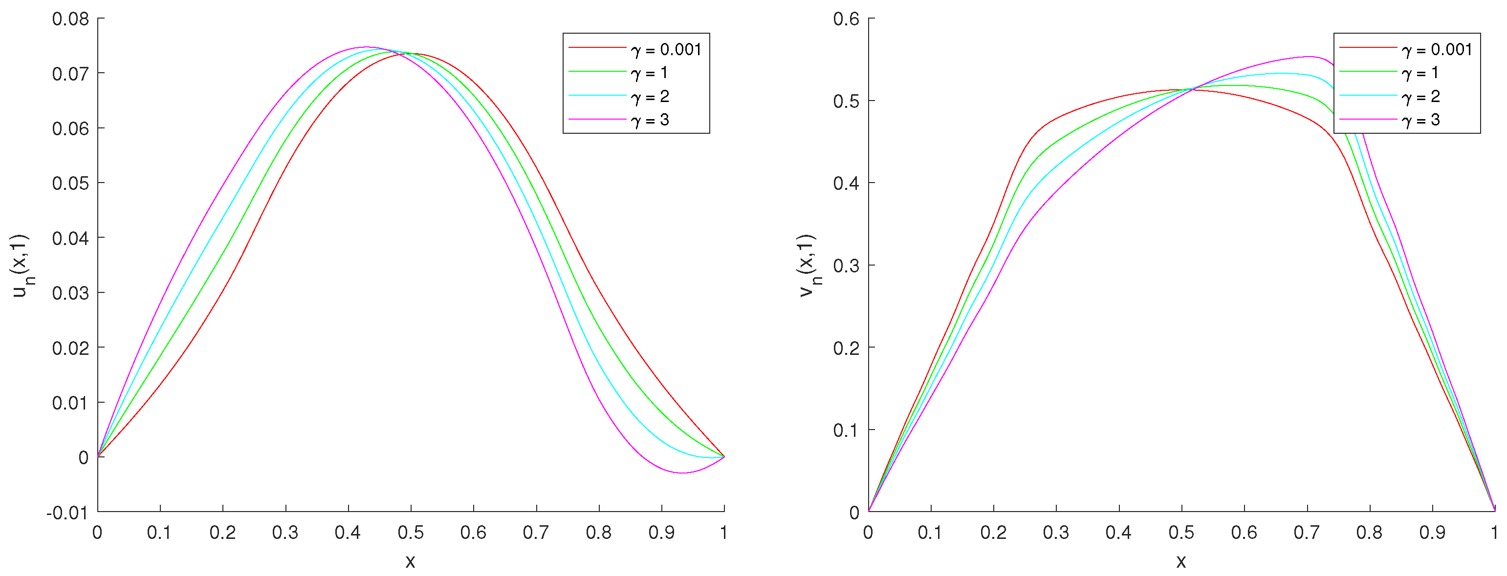
4.2. Dependence of the Solution on the Coupling Parameter $\gamma$

In this last example, we will investigate the dependence on the coupling parameter $\gamma$ for the solution to the thermomechanical problem (1)–(3).

Again, we suppose that the supply terms vanish and we employ the data:

$$\begin{array}{c}T=1,\ell =1,{\rho }_z=1,{\rho }_u=5,{\alpha }_1=4,{\alpha }_2=1,{\alpha }_3=3,\hfill \\ {\rho }_{\theta }=200,\tau =100,\beta =40.\hfill \end{array}$$

If we consider the initial conditions given by

$$\begin{array}{c}\hfill u_0\left(x\right)=v_0\left(x\right)=z_0\left(x\right)=y_0\left(x\right)={\theta }_0\left(x\right)=q_0\left(x\right)=x(x-1)\forall x\in (0,1),\end{array}$$

using the values $h=0.01$ and $k=0.0001$ the solution to discrete problem (13)–(17) is plotted in Figure 3 and Figure 4 for some values of parameter $\gamma$. From these pictures, we can conclude that this parameter has no influence in the displacement of the fluid and the heat flux, and that the differences are very small for the temperature and the velocity of the fluid Figure 5. However, there is an important difference in the displacement and velocity of the solid. It seems that a time delay is generated depending on the value of $\gamma$.

5. Conclusions

In this work, we have analyzed, from the numerical point of view, a one-dimensional problem involving swelling materials with the so-called second sound effect.

First, we derived the variational form of the linear system studied in [25] after integration by parts, and we introduced a fully discrete approximation by using the classical finite element method with linear elements and the backward Euler scheme. We proved the discrete stability of the resulting approximations and we showed an a priori error analysis. After the implementation of the algorithm in MATLAB, we performed some numerical simulations. In the first example, we demonstrated the linear convergence of the approximations and, from the curve of the discrete energy, we showed the theoretical exponential energy decay. Then, in the final example, we considered the dependence on the coupling parameter between the displacements and the temperature.

References

1. Karalis, T.K. On the elastic deformation of non-saturated swelling soils. Acta Mech. 1990, 84, 19–45. [Google Scholar] [CrossRef]
2. Philip, J.R. Hydrostatics and hydrodynamics in swelling soils. Water Resour. Res. 1969, 5, 1070–1077. [Google Scholar] [CrossRef]
3. Sposito, G. Thermodynamics of swelling clay-water systems. Soil Sci. 1972, 114, 243–249. [Google Scholar] [CrossRef]
4. Bowen, R.M.; Wiese, J.C. Diffusion in mixtures of elastic materials. Int. J. Eng. Sci. 1969, 7, 689–722. [Google Scholar] [CrossRef]
5. Bowen, R.M. Theory of Mixtures in Continuum Physics. In Continuum Physics, Mixtures and EM Field Theories; Academic Press: New York, NY, USA, 1976; Volume III, pp. 1–127. [Google Scholar]
6. Ieşan, D.; Quintanilla, R. Existence and continuous dependence results in the theory of interacting continua. J. Elasticity 1994, 36, 85–98. [Google Scholar] [CrossRef]
7. Quintanilla, R. Exponential stability for one-dimensional problem of swelling porous elastic soils with fluid saturation. J. Comput. Appl. Math. 2002, 145, 525–533. [Google Scholar] [CrossRef]
8. Eringen, A.C. A continuum theory of swelling porous elastic solids. Int. J. Eng. Sci. 1994, 332, 1337–1349. [Google Scholar] [CrossRef]
9. Al-Mahdi, A.M.; Al-Gharabli, M.M.; Alahyane, M. Theoretical and numerical stability results for a viscoelastic swelling porous-elastic system with past history. AIMS Math. 2021, 6, 11921–11949. [Google Scholar] [CrossRef]
10. Apalara, T.A.; Almutairi, O.B. Well-Posedness and Exponential Stability of Swelling Porous with Gurtin–Pipkin Thermoelasticity. Mathematics 2022, 10, 4498. [Google Scholar] [CrossRef]
11. Almeida Júnior, D.S.; Ramos, A.J.A.; Noé, A.S.; Freitas, M.M.; Aum, P.T.P. Stabilization and numerical treatment for swelling porous elastic soils with fluid saturation. Z. Angew. Math. Phys. 2021, 101, e202000366. [Google Scholar]
12. Apalara, T.A.; Yusuf, M.O.; Salami, B.A. On the control of viscoelastic damped swelling porous elastic soils with internal delay feedbacks. J. Math. Anal. Appl. 2021, 504, 125429. [Google Scholar] [CrossRef]
13. Apalara, T.A. General stability result of swelling porous elastic soils with a viscoelastic damping. Z. Angew. Math. Phys. 2020, 71, 200. [Google Scholar] [CrossRef]
14. Chiriţă, S. On the spatial decay of solutions in the theory of swelling porous thermoelastic soils. Internat. J. Engrg. Sci. 2004, 42, 1995–2010. [Google Scholar] [CrossRef]
15. Freitas, M.M.; Ramos, A.J.A.; Santos, M.L. Existence and upper-semicontinuity of global attractors for binary mixtures solids with fractional damping. Appl. Math. Optim. 2021, 83, 1353–1383. [Google Scholar] [CrossRef]
16. Freitas, M.M.; Ramos, A.J.A.; Almeida Júnior, D.S.; Miranda, L.G.R.; Noé, A.S. Asymptotic dynamics for fractionally damped swelling porous elastic soils with memory. Boll. Unione Mat. Ital. 2023, 16, 1–23. [Google Scholar] [CrossRef]
17. Galeş, C. Potential method in the linear theory of swelling porous elastic soils. Eur. J. Mech. A Solids 2004, 23, 957–973. [Google Scholar] [CrossRef]
18. Kalantari, B. Engineering significant of swelling soils. Res. J. Appl. Sci. Eng. Technol. 2012, 4, 2874–2878. [Google Scholar]
19. Kumar, R.; Batra, D. Fundamental solution of steady oscillation in swelling porous thermoelastic medium. Acta Mech. 2020, 231, 3247–3263. [Google Scholar] [CrossRef]
20. Nonato, C.A.S.; Ramos, A.J.A.; Raposo, C.A.; Dos Santos, M.J.; Freitas, M.M. Stabilization of swelling porous elastic soils with fluid saturation, time varying-delay and time-varying weights. Z. Angew. Math. Phys. 2022, 73, 20. [Google Scholar] [CrossRef]
21. Ramos, A.J.A.; Apalara, T.A.; Freitas, M.M.; Araújo, M.L. Equivalence between exponential stabilization and boundary observability for swelling problem. J. Math. Phys. 2022, 63, 011511. [Google Scholar] [CrossRef]
22. Tomar, S.K.; Goyal, S. Elastic waves in swelling porous media. Transp. Porous Media 2013, 100, 39–68. [Google Scholar] [CrossRef]
23. Wang, J.M.; Guo, B.Z. On the stability of swelling porous elastic soils with fluid saturation by one internal damping. IMA J. Appl. Math. 2006, 71, 565–582. [Google Scholar] [CrossRef]
24. Youkana, A.; Al-Mahdi, A.M.; Messaoudi, S.A. General energy decay result for a viscoelastic swelling porous-elastic system. Z. Angew. Math. Phys. 2022, 73, 88. [Google Scholar] [CrossRef]
25. Apalara, T.A.; Soufyane, A.; Mounir, A. On well-posedness and exponential decay of swelling porous thermoelastic media with second sound. J. Math. Anal. Appl. 2022, 510, 126006. [Google Scholar] [CrossRef]
26. Ciarlet, P.G. Basic error estimates for elliptic problems. In Handbook of Numerical Analysis. Vol. II; Elsevier Science Publishers B.V.: North-Holland, The Netherlands, 1991; pp. 17–352. [Google Scholar]
27. Campo, M.; Fernández, J.; Kuttler, K.; Shillor, M.; Viaño, J. Numerical analysis and simulations of a dynamic frictionless contact problem with damagen. Comput. Methods Appl. Mech. Eng. 2006, 196, 476–488. [Google Scholar] [CrossRef]
Figure 1. Example 1: asymptotic constant error.
Mathematics 11 01456 g001
Figure 2. Example 1: evolution of the discrete energy along time in both natural and semi-log scales.
Mathematics 11 01456 g002
Figure 3. Example 2: displacement and velocity of the elastic solid for different values of parameter γ .
Mathematics 11 01456 g003
Figure 4. Example 2: displacement and velocity of the fluid for different values of parameter γ .
Mathematics 11 01456 g004
Figure 5. Example 2: temperature and heat flux for different values of parameter γ .
Mathematics 11 01456 g005