

Optimal Strategy for Comfort-Based Home Energy Management System Considering Impact of Battery Degradation Cost Model

 , , ,
, , ,  ,
, 

Abstract
:1. Introduction
- A mixed objective MIP model of HEMS is formulated to minimize household energy consumption costs and satisfy residents’ thermal comfort in daily life by integrating the PV panel, HESS, and PEV, keeping load profiling to the limitation of the utility and combining the users’ comfort requirements of both AC and EWH in the framework;
- Two types of battery degradation costs for the HESS and PEV are taken into account in the battery charging and discharging scheduling strategy, considering the impact of RTP and technical constraints. These additions not only guarantee the lowest cost and user’s comfort but also manage the energy transaction reasonably between the residence and utility and prolong the service life of the batteries.
2. System Modeling
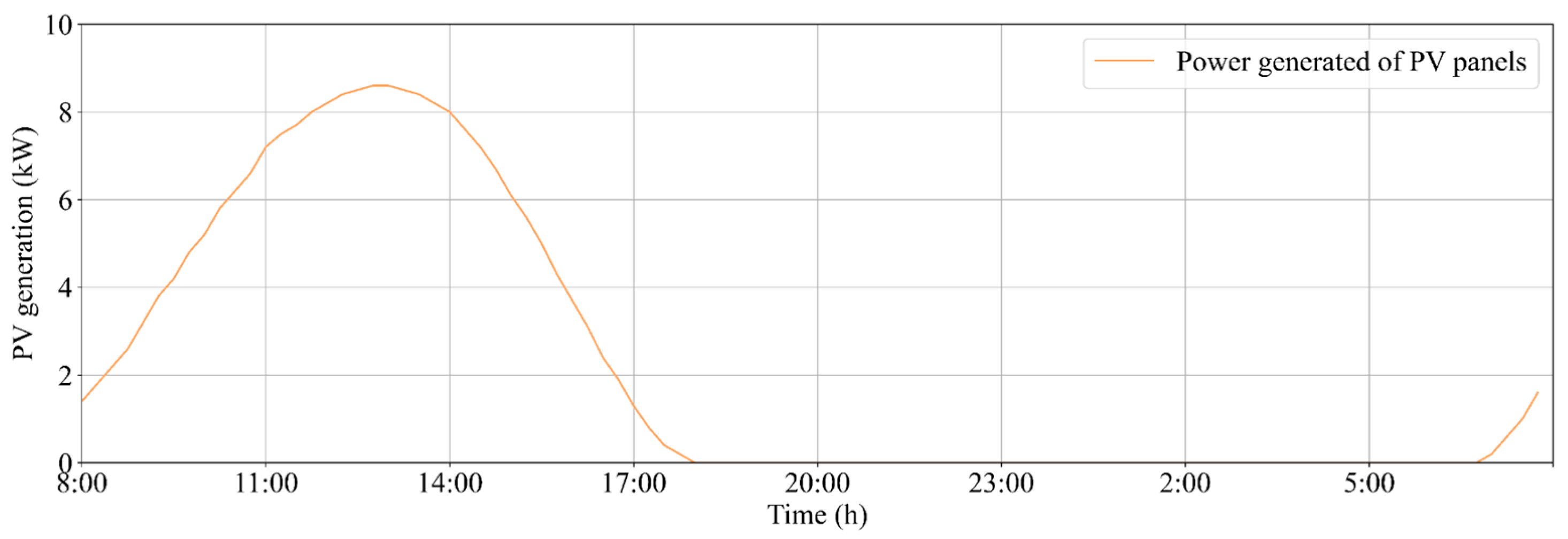
2.1. PV Panels
2.2. Home Appliances
2.3. HESS
2.4. PEV
2.5. Utility
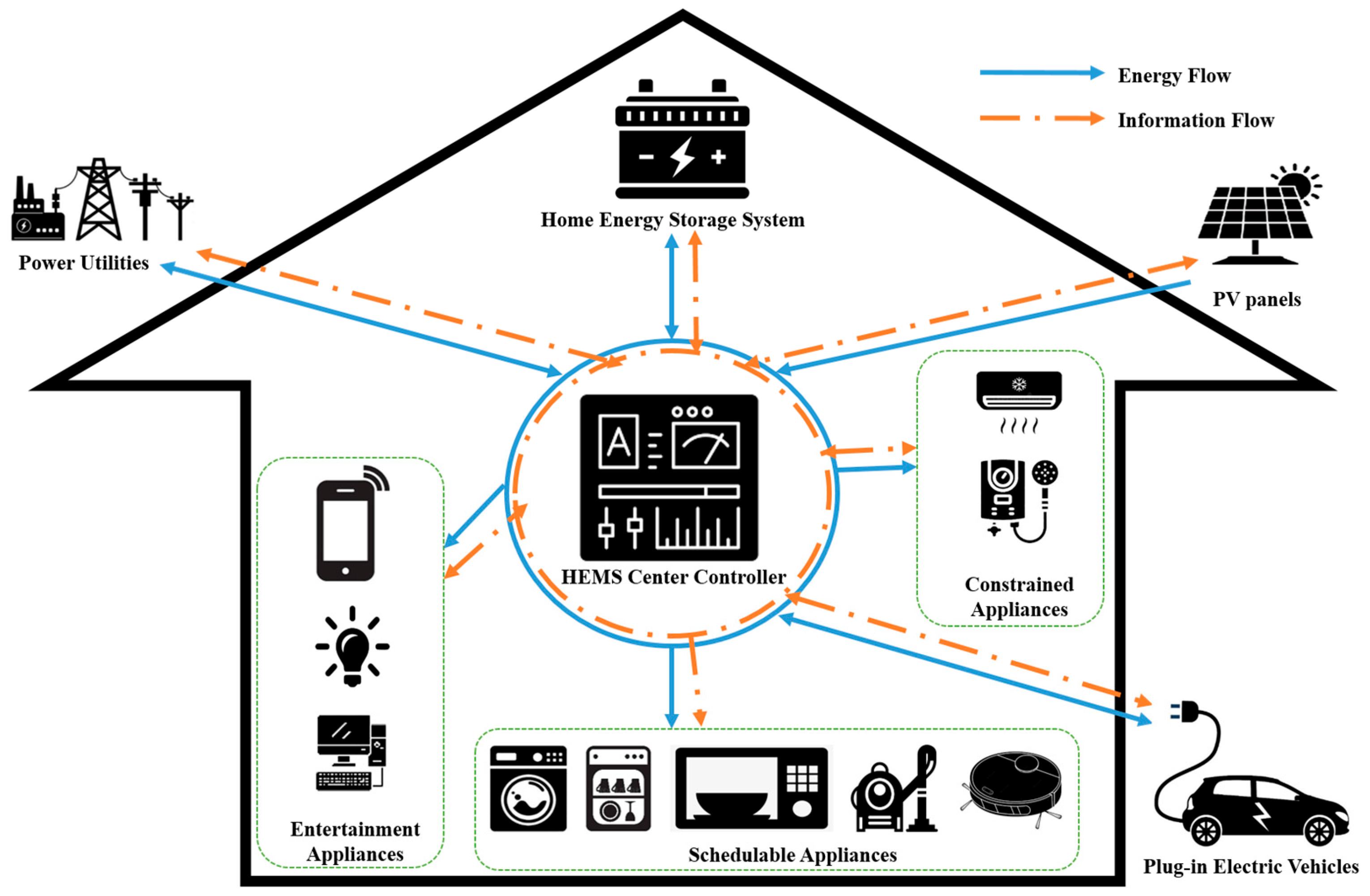
2.6. Central Controller
3. Proposed Method
3.1. Quadratic Model of the Battery Degradation
3.2. Reciprocal Model of the Battery Degradation
3.3. Charging and Discharging Strategy
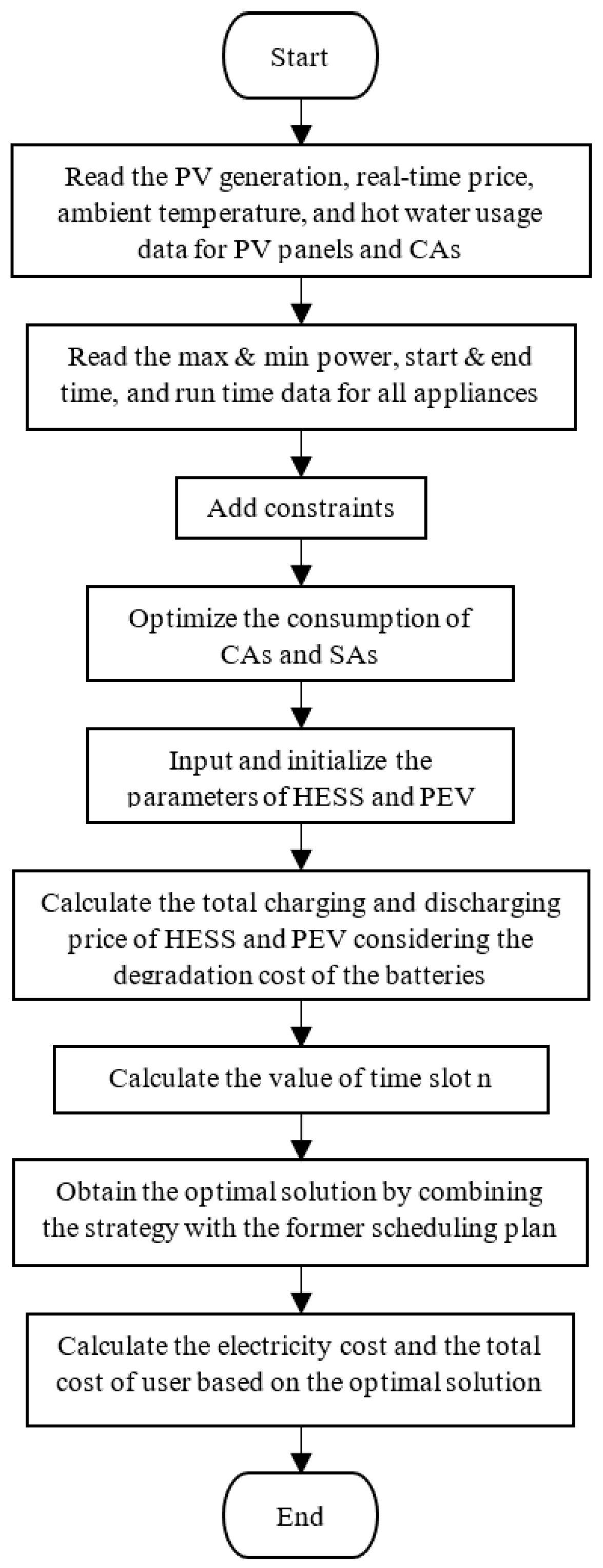
3.4. Optimization Algorithms
4. Results and Discussion
4.1. Appliances Scheduling Results
4.2. Case Study
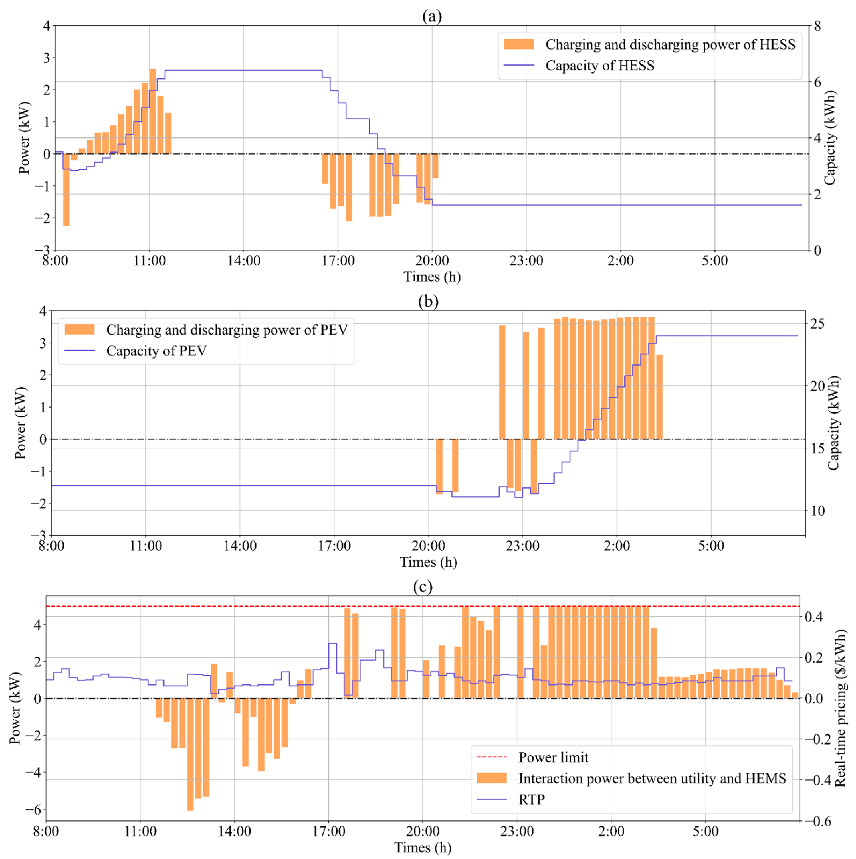
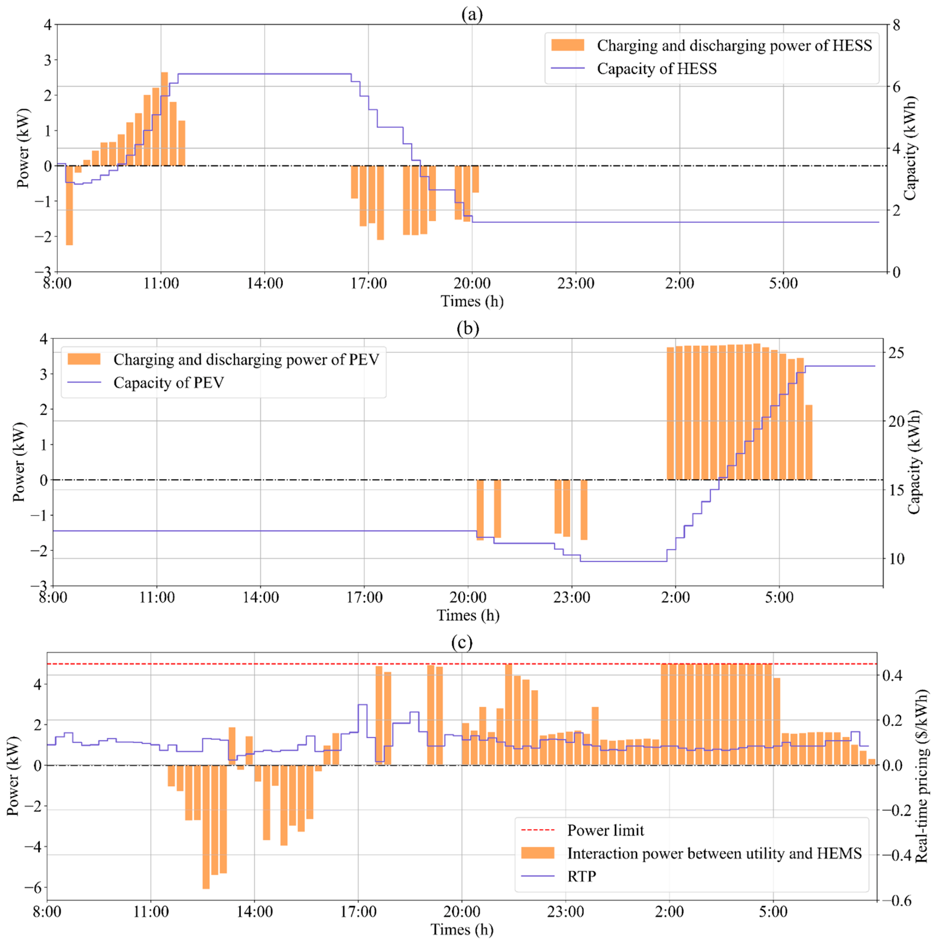
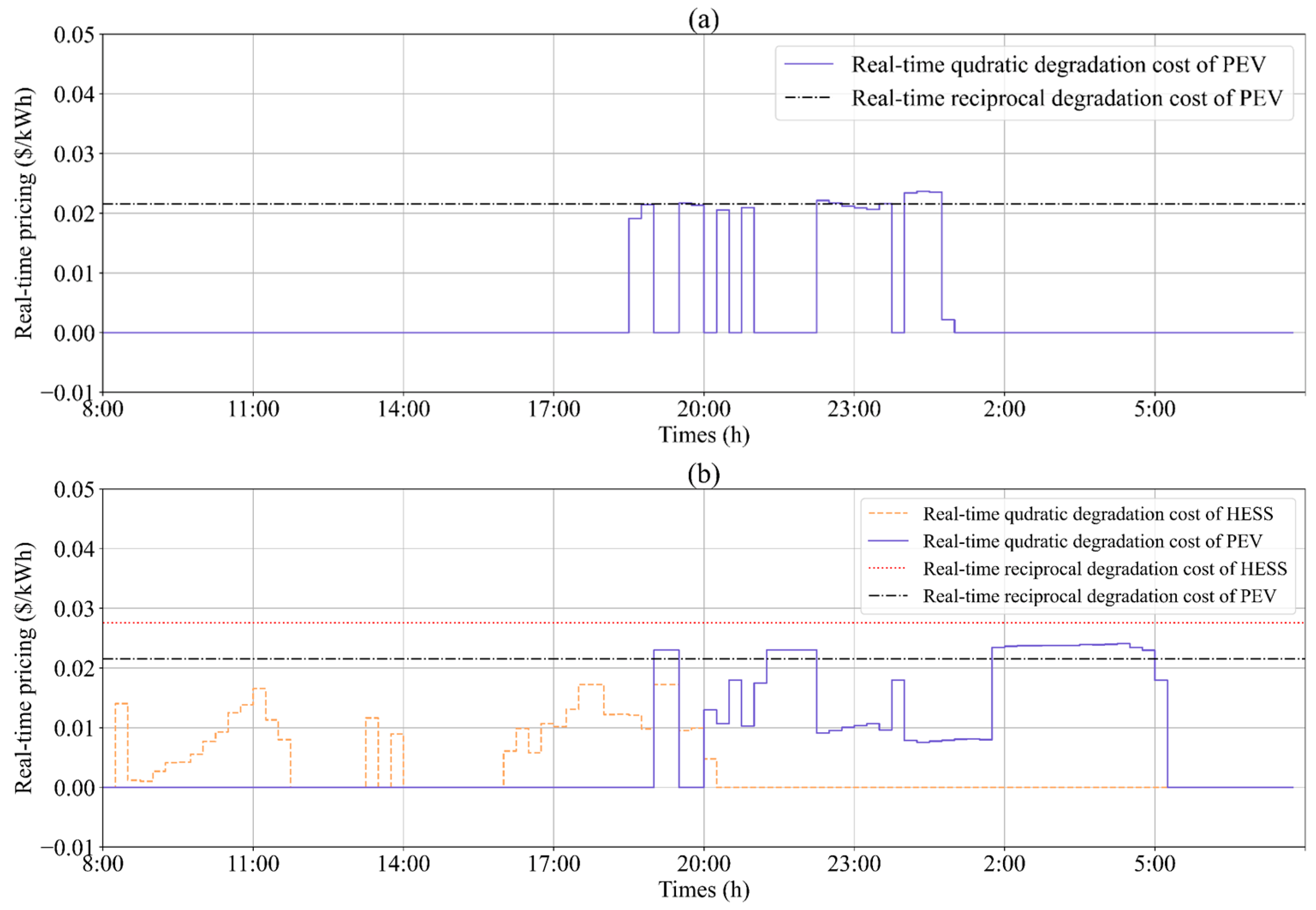
4.2.1. HEMSs with Quadratic Model of Degradation Cost
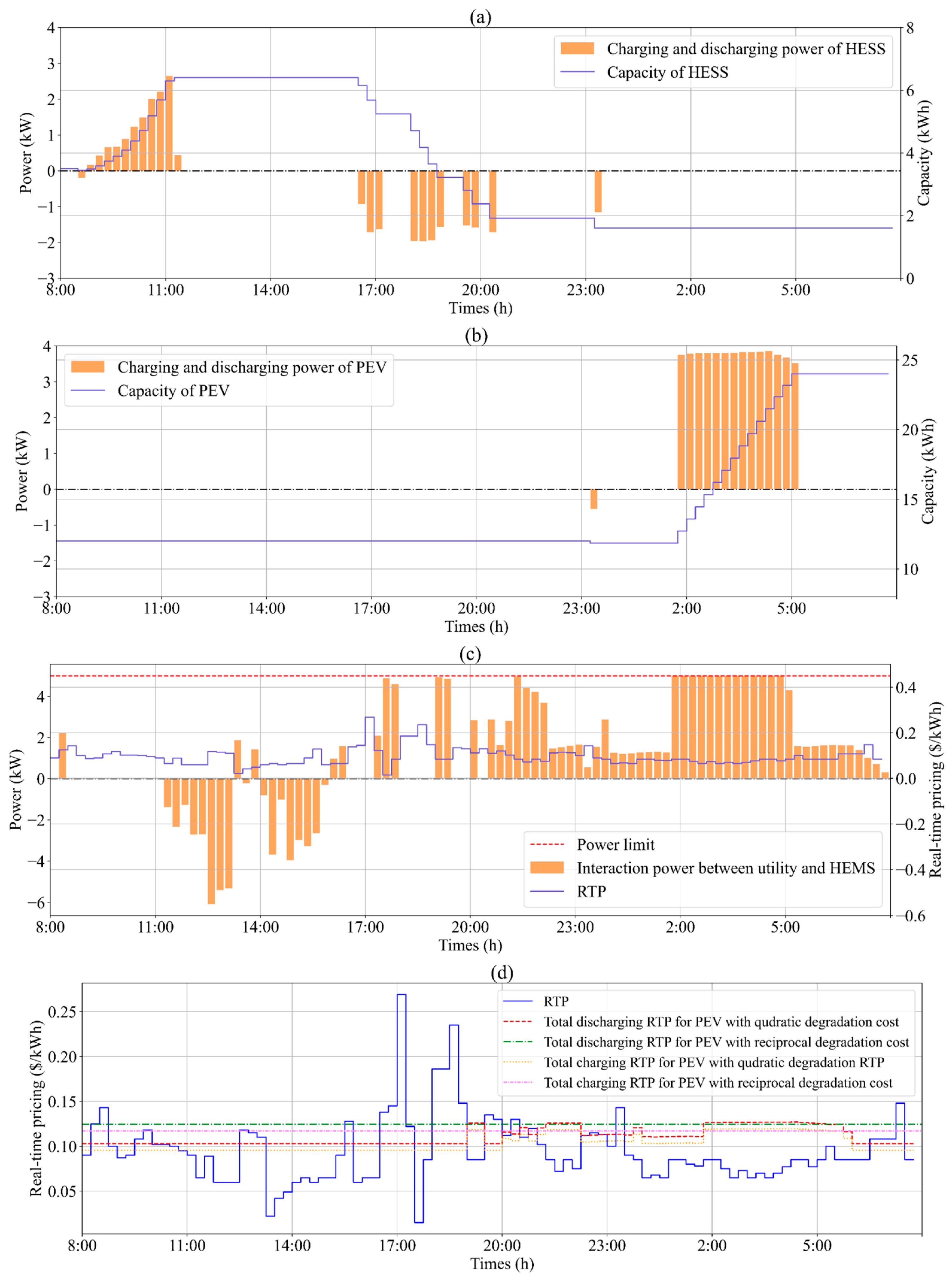
4.2.2. HEMSs with Reciprocal Model of Degradation Cost
4.3. Sensitivity Analysis
4.4. Modeling Error Analysis
4.5. Other Findings and Limitations
- Installing HESS in the home leads to decreasing the cost of energy and making full use of the power generated by the PV panels;
- The change of the operation mode of PEV and the combination of the proposed charging and discharging strategy of batteries improve the efficiency of the PV-integrated HEMS and decrease the electricity cost and total cost;
- The addition of the degradation cost has an influence on the charging and discharging behavior of HESS and PEV batteries, and a fully equipped HEMS with a suitable degradation cost model (Case 4) leads to the best optimization plan between the cases.
- It is assumed that the everyday arrival and departure time of PEV are fixed in this study, which cannot be reached in reality, and the uncertainty of the arrival and departure time of PEV can be taken into account in the future simulations;
- The quadratic model of degradation cost is simple to calculate but does not consider the investment cost of batteries, which can affect the results of simulations;
- The investment cost of batteries is included in the reciprocal degradation cost model; however, the parameters of batteries for HESS and PEV are assumed to be fixed in this work, which are, in fact, changeable during the daily use of HESS and PEV and can slightly change the results;
- The selling price of energy is assumed to be 50% of the buying price of the utility. In reality, the selling price of energy is not always related to the buying price of the utility and is often affected by the financial incentives proposed by utilities.
5. Conclusions
Author Contributions
Funding
Data Availability Statement
Conflicts of Interest
Nomenclature
| Abbreviations | |
| AC | Air conditioning |
| CA | Constrained appliance |
| CPP | Critical peak pricing |
| DR | Demand response |
| EA | Entertainment appliance |
| EWH | Electric water heater |
| G2V | Grid-to-vehicle |
| HEMS | Home energy management system |
| HESS | Home energy storage system |
| HESS2H | HESS-to-home |
| H-MG | Home micro-grid |
| IBR | Inclining block rates |
| MIP | Mixed integer programming |
| PAR | Peak-to-average ratio |
| PEV | Plug-in electric vehicle |
| PV | Photovoltaic |
| RESs | Renewable energy sources |
| SA | Schedulable appliance |
| SG | Smart grid |
| TOU | Time-of-use |
| V2H | Vehicle-to-home |
| Sets and indices | |
| T | Set of time slots |
| t | Index of time slots |
| S | Set of SA loads |
| s | Index of SA loads |
| Parameters | |
| PV surface area | |
| Maximum capacity of the batteries used in HESS | |
| Initial capacity of the batteries used in HESS | |
| Lifetime in cycles of the batteries used in HESS | |
| Maximum capacity of the batteries used in PEV | |
| Initial capacity of the batteries used in PEV | |
| Lifetime in cycles of the batteries used in PEV | |
| Depth of discharge of the batteries used in HESS | |
| Depth of discharge of the batteries used in PEV | |
| Number of time intervals that appliances need to fulfill their tasks | |
| Power consumption of EA loads | |
| Maximum power drawn from the utility | |
| Maximum charging power of the batteries used in HESS | |
| Maximum discharging power of the batteries used in HESS | |
| Power of the load | |
| Maximum charging power of the batteries used in PEV | |
| Maximum discharging power of the batteries used in PEV | |
| PV generation | |
| Q | Energy input rate |
| Solar irradiance | |
| Replacement cost including labor of the batteries used in HESS | |
| Replacement cost including labor of the batteries used in PEV | |
| Real-time discharging pricing of the batteries used in HESS | |
| Real-time charging pricing of the batteries used in PEV | |
| Real-time discharging pricing of the batteries used in PEV | |
| Surface coefficient | |
| Arrival time of PEV | |
| Departure time of PEV | |
| Start time of the load | |
| End time of the load | |
| Time interval (15 min) | |
| α, β | Thermal characteristics of air conditioning |
| Charging and discharging efficiency of the batteries used in HESS | |
| Charging and discharging efficiency of the batteries used in PEV | |
| Efficiency of PV | |
| Variables | |
| Capacity of the batteries used in HESS | |
| Degradation cost of HESS and PEV | |
| Capacity of the batteries used in PEV | |
| Power of air conditioning | |
| Power of electric water heater | |
| The interaction power between the utility and H-MG | |
| Power of HESS | |
| Charging power of HESS | |
| Maximum chargeable power of HESS | |
| Discharging power of HESS | |
| Maximum dischargeable power of HESS | |
| Power of PEV | |
| Charging power of PEV | |
| Maximum chargeable power of PEV | |
| Discharging power of PEV | |
| Maximum dischargeable power of PEV | |
| Running state of SA loads (binary variable: 1 for charging and 0 for discharging) | |
| Running state of HESS (binary variable: 1 for charging and 0 for discharging) | |
| Running state of PEV (binary variable: 1 for charging and 0 for discharging) | |
References
- Han, B.; Zahraoui, Y.; Mubin, M.; Mekhilef, S.; Seyedmahmoudian, M.; Stojcevski, A. Home Energy Management Systems : A Review of the Concept, Architecture, and Scheduling Strategies. IEEE Access 2023, 11, 19999–20025. [Google Scholar] [CrossRef]
- Zahraoui, Y.; Alhamrouni, I.; Mekhilef, S.; Reyasudin Basir Khan, M.; Seyedmahmoudian, M.; Stojcevski, A.; Horan, B. Energy management system in microgrids: A comprehensive review. Sustainability 2021, 13, 10492. [Google Scholar] [CrossRef]
- Hou, Q.; Zhang, N.; Du, E.; Miao, M.; Peng, F.; Kang, C. Probabilistic duck curve in high PV penetration power system: Concept, modeling, and empirical analysis in China. Appl. Energy 2019, 242, 205–215. [Google Scholar] [CrossRef]
- Zahraoui, Y.; Alhamrouni, I.; Basir Khan, M.R.; Mekhilef, S.; Hayes, B.P.; Rawa, M.; Ahmed, M. Self-healing strategy to enhance microgrid resilience during faults occurrence. Int. Trans. Electr. Energy Syst. 2021, 31, 13232. [Google Scholar] [CrossRef]
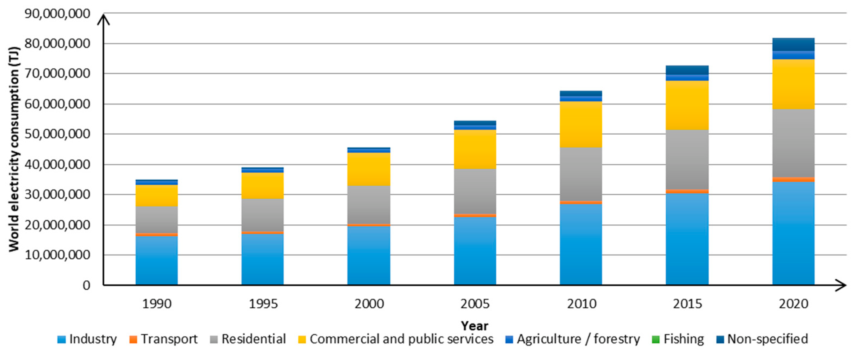
- International Energy Agency (IEA) World Energy Balances. 2022. Available online: https://www.iea.org/data-and-statistics/data-tools/energy-statistics-data-browser?country=WORLD&fuel=Energyconsumption&indicator=ElecConsBySector (accessed on 26 January 2023).
- Elkazaz, M.; Sumner, M.; Pholboon, S.; Davies, R.; Thomas, D. Performance assessment of an energy management system for a home microgrid with PV generation. Energies 2020, 13, 3436. [Google Scholar] [CrossRef]
- Samadi, A.; Saidi, H.; Latify, M.A.; Mahdavi, M. Home energy management system based on task classification and the resident’s requirements. Int. J. Electr. Power Energy Syst. 2020, 118, 105815. [Google Scholar] [CrossRef]
- Luo, J.T.; Joybari, M.M.; Panchabikesan, K.; Sun, Y.; Haghighat, F.; Moreau, A.; Robichaud, M. Performance of a self-learning predictive controller for peak shifting in a building integrated with energy storage. Sustain. Cities Soc. 2020, 60, 102285. [Google Scholar] [CrossRef]
- Javadi, M.S.; Gough, M.; Lotfi, M.; Esmaeel Nezhad, A.; Santos, S.F.; Catalão, J.P.S. Optimal self-scheduling of home energy management system in the presence of photovoltaic power generation and batteries. Energy 2020, 210, 118568. [Google Scholar] [CrossRef]
- Duman, A.C.; Erden, H.S.; Gönül, Ö.; Güler, Ö. A home energy management system with an integrated smart thermostat for demand response in smart grids. Sustain. Cities Soc. 2021, 65, 102639. [Google Scholar] [CrossRef]
- Beaudin, M.; Zareipour, H. Home energy management systems: A review of modelling and complexity. Renew. Sustain. Energy Rev. 2015, 45, 318–335. [Google Scholar] [CrossRef]
- Moen, R.L. Solar Energy Management System. In Proceedings of the Proceedings of the IEEE Conference on Decision and Control, Fort Lauderdale, FL, USA, 12–14 December 1979; Volume 2, pp. 917–919. [Google Scholar]
- Zahraoui, Y.; Alhamrouni, I.; Mekhilef, S.; Basir Khan, M.R.; Hayes, B.P.; Ahmed, M. A novel approach for sizing battery storage system for enhancing resilience ability of a microgrid. Int. Trans. Electr. Energy Syst. 2021, 31, e13142. [Google Scholar] [CrossRef]
- Alsharif, A.; Tan, C.W.; Ayop, R.; Dobi, A.; Lau, K.Y. A comprehensive review of energy management strategy in Vehicle-to-Grid technology integrated with renewable energy sources. Sustain. Energy Technol. Assess. 2021, 47, 101439. [Google Scholar] [CrossRef]
- Ben Arab, M.; Rekik, M.; Krichen, L. Suitable various-goal energy management system for smart home based on photovoltaic generator and electric vehicles. J. Build. Eng. 2022, 52, 104430. [Google Scholar] [CrossRef]
- Capehart, B.L.; Muth, E.J.; Storin, M.O. Minimizing residential electrical energy costs using microcomputer energy management systems. Comput. Ind. Eng. 1982, 6, 261–269. [Google Scholar] [CrossRef]
- Hensgen, D.A.; Kidd, T.; St. John, D.; Schnaidt, M.C.; Siegel, H.J.; Braun, T.D.; Maheswaran, M.; Ali, S.; Kim, J.K.; Irvine, C.; et al. An overview of MSHN: The management system for heterogeneous networks. In Proceedings of the Heterogeneous Computing Workshop, Washington, DC, USA, 12 April 1999; pp. 184–198. [Google Scholar]
- Tostado-Véliz, M.; Gurung, S.; Jurado, F. Efficient solution of many-objective Home Energy Management systems. Int. J. Electr. Power Energy Syst. 2022, 136, 107666. [Google Scholar] [CrossRef]
- Gholami, M.; Sanjari, M.J. Multiobjective energy management in battery-integrated home energy systems. Renew. Energy 2021, 177, 967–975. [Google Scholar] [CrossRef]
- Merdanoğlu, H.; Yakıcı, E.; Doğan, O.T.; Duran, S.; Karatas, M. Finding optimal schedules in a home energy management system. Electr. Power Syst. Res. 2020, 182, 106229. [Google Scholar] [CrossRef]
- Mansouri, S.A.; Ahmarinejad, A.; Nematbakhsh, E.; Javadi, M.S.; Jordehi, A.R.; Catalão, J.P.S. Energy management in microgrids including smart homes: A multi-objective approach. Sustain. Cities Soc. 2021, 69, 102852. [Google Scholar] [CrossRef]
- Mak, D.; Choi, D.H. Optimization framework for coordinated operation of home energy management system and Volt-VAR optimization in unbalanced active distribution networks considering uncertainties. Appl. Energy 2020, 276, 115495. [Google Scholar] [CrossRef]
- Lu, Q.; Zhang, Z.; Lü, S. Home energy management in smart households: Optimal appliance scheduling model with photovoltaic energy storage system. Energy Rep. 2020, 6, 2450–2462. [Google Scholar] [CrossRef]
- Shakeri, M.; Shayestegan, M.; Reza, S.M.S.; Yahya, I.; Bais, B.; Akhtaruzzaman, M.; Sopian, K.; Amin, N. Implementation of a novel home energy management system (HEMS) architecture with solar photovoltaic system as supplementary source. Renew. Energy 2018, 125, 108–120. [Google Scholar] [CrossRef]
- Esmaeel Nezhad, A.; Rahimnejad, A.; Gadsden, S.A. Home energy management system for smart buildings with inverter-based air conditioning system. Int. J. Electr. Power Energy Syst. 2021, 133, 107230. [Google Scholar] [CrossRef]
- Javadi, M.S.; Nezhad, A.E.; Gough, M.; Lotfi, M.; Anvari-Moghaddam, A.; Nardelli, P.H.J.; Sahoo, S.; Catalão, J.P.S. Conditional Value-at-Risk Model for Smart Home Energy Management Systems. e-Prime 2021, 1, 100006. [Google Scholar] [CrossRef]
- Langer, L.; Volling, T. An optimal home energy management system for modulating heat pumps and photovoltaic systems. Appl. Energy 2020, 278, 115661. [Google Scholar] [CrossRef]
- Younes, Z.; Alhamrouni, I.; Mekhilef, S.; Reyasudin, M. A memory-based gravitational search algorithm for solving economic dispatch problem in micro-grid. Ain Shams Eng. J. 2021, 12, 1985–1994. [Google Scholar] [CrossRef]
- Zupančič, J.; Filipič, B.; Gams, M. Genetic-programming-based multi-objective optimization of strategies for home energy-management systems. Energy 2020, 203, 117769. [Google Scholar] [CrossRef]
- Mehrjerdi, H. Peer-to-peer home energy management incorporating hydrogen storage system and solar generating units. Renew. Energy 2020, 156, 183–192. [Google Scholar] [CrossRef]
- Park, H. Human comfort-based-home energy management for demand response participation. Energies 2020, 13, 2463. [Google Scholar] [CrossRef]
- Wang, X.; Mao, X.; Khodaei, H. A multi-objective home energy management system based on internet of things and optimization algorithms. J. Build. Eng. 2021, 33, 101603. [Google Scholar] [CrossRef]
- Jin, X.; Baker, K.; Christensen, D.; Isley, S. Foresee: A user-centric home energy management system for energy efficiency and demand response. Appl. Energy 2017, 205, 1583–1595. [Google Scholar] [CrossRef]
- Javadi, M.S.; Nezhad, A.E.; Nardelli, P.H.J.; Gough, M.; Lotfi, M.; Santos, S.; Catalão, J.P.S. Self-scheduling model for home energy management systems considering the end-users discomfort index within price-based demand response programs. Sustain. Cities Soc. 2021, 68, 102792. [Google Scholar] [CrossRef]
- Bayram, I.S.; Ustun, T.S. A survey on behind the meter energy management systems in smart grid. Renew. Sustain. Energy Rev. 2017, 72, 1208–1232. [Google Scholar] [CrossRef]
- Zahraoui, Y.; Korõtko, T.; Rosin, A.; Agabus, H. Market Mechanisms and Trading in Microgrid Local Electricity Markets: A Comprehensive Review. Energies. 2023, 16, 2145. [Google Scholar] [CrossRef]
- Esther, B.P.; Kumar, K.S. A survey on residential Demand Side Management architecture, approaches, optimization models and methods. Renew. Sustain. Energy Rev. 2016, 59, 342–351. [Google Scholar] [CrossRef]
- Sharifi, A.H.; Maghouli, P. Energy management of smart homes equipped with energy storage systems considering the PAR index based on real-time pricing. Sustain. Cities Soc. 2019, 45, 579–587. [Google Scholar] [CrossRef]
- Ben Slama, S. Design and implementation of home energy management system using vehicle to home (H2V) approach. J. Clean. Prod. 2021, 312, 127792. [Google Scholar] [CrossRef]
- Zahraoui, Y.; Alhamrouni, I.; Mekhilef, S.; Basir Khan, M.R. Chapter one—Machine learning algorithms used for short-term PV solar irradiation and temperature forecasting at microgrid. In Applications of AI and IOT in Renewable Energy; Shaw, R.N., Ghosh, A., Mekhilef, S., Balas, V.E., Eds.; Academic Press: Cambridge, MA, USA, 2022; pp. 1–17. ISBN 978-0-323-91699-8. [Google Scholar]
- Zahraoui, Y.; Alhamrouni, I.; Hayes, B.P.; Mekhilef, S.; Korõtko, T. System-Level Condition Monitoring Approach for Fault Detection in Photovoltaic Systems. In Fault Analysis and its Impact on Grid-connected Photovoltaic Systems Performance; John Wiley & Sons, Ltd.: Hoboken, NJ, USA, 2022; pp. 215–254. ISBN 9781119873785. [Google Scholar]
- Hou, X.; Wang, J.; Huang, T.; Wang, T.; Wang, P. Smart Home Energy Management Optimization Method Considering Energy Storage and Electric Vehicle. IEEE Access 2019, 7, 144010–144020. [Google Scholar] [CrossRef]
- Li, N.; Chen, L.; Low, S.H. Optimal demand response based on utility maximization in power networks. In Proceedings of the 2011 IEEE Power and Energy Society General Meeting, Detroit, MI, USA, 24–28 July 2011. [Google Scholar]
- Nehrir, M.H.; Jia, R.; Pierre, D.A.; Hammerstrom, D.J. Power management of aggregate electric water heater loads by voltage control. In Proceedings of the 2007 IEEE Power Engineering Society General Meeting, Tampa, FL, USA, 24–28 June 2007. [Google Scholar]
- Liu, Y.; Li, Y.; Gooi, H.B.; Jian, Y.; Xin, H.; Jiang, X.; Pan, J. Distributed Robust Energy Management of a Multimicrogrid System in the Real-Time Energy Market. IEEE Trans. Sustain. Energy 2019, 10, 396–406. [Google Scholar] [CrossRef]
- Khan, M.W.; Wang, J. Multi-agents based optimal energy scheduling technique for electric vehicles aggregator in microgrids. Int. J. Electr. Power Energy Syst. 2022, 134, 107346. [Google Scholar] [CrossRef]
- The Australian Energy Market Operator (AEMO) Metadata. Available online: https://aemo.com.au/ (accessed on 27 October 2022).
- Du, P.; Lu, N. Appliance commitment for household load scheduling. IEEE Trans. Smart Grid 2011, 2, 411–419. [Google Scholar] [CrossRef]


| Category | Appliances | Max Power (kW) | Min Power (kW) | Start Time | End Time | Running Time (h) |
|---|---|---|---|---|---|---|
| EA | Light, Television, Phone, Computer | 1 | 1 | 8:00 | 8:00 | 24 |
| CA | Air Conditioning | 3 | 0 | 8:00 | 8:00 | 24 |
| CA | Electric Water Heater | 3.5 | 0 | 8:00 | 8:00 | 24 |
| SA | Washing Machine | 1.5 | 1.5 | 9:00 | 22:00 | 1 |
| SA | Washing Machine | 1.5 | 1.5 | 10:00 | 0:00 | 2 |
| SA | Dishwasher | 1.2 | 1.2 | 10:00 | 15:00 | 2 |
| SA | Dishwasher | 1.2 | 1.2 | 18:00 | 22:00 | 2 |
| SA | Hairdryer | 1.8 | 1.8 | 8:00 | 23:00 | 0.25 |
| SA | Vacuum Cleaner | 1.2 | 1.2 | 14:00 | 18:00 | 0.5 |
| SA | Rice Cooker | 0.8 | 0.8 | 10:00 | 12:00 | 0.75 |
| SA | Rice Cooker | 0.8 | 0.8 | 16:00 | 19:00 | 0.75 |
| SA | Oven | 2 | 2 | 10:00 | 19:00 | 2 |
| SA | Humidifier | 0.15 | 0.15 | 8:00 | 0:00 | 4 |
| SA | Robot Vacuum Cleaner | 0.7 | 0.7 | 8:00 | 0:00 | 5 |
| Parameters for Indoor Temperature Calculation | Parameters for Hot Water Temperature Calculation | ||
|---|---|---|---|
| 80 | 150 | ||
| 73 | 120 | ||
| 77 | 70 | ||
| α | 0.9 | 70 | |
| β | −11 | 80 | |
| Parameters for HESS | Parameters for PEV | ||
|---|---|---|---|
| 8 | 30 | ||
| 3.5 | 12 | ||
| 3 | 4 | ||
| −3 | −4 | ||
| 0.92 | 0.92 | ||
| 70 | 80 | ||
| 1250 | 2000 | ||
| 695 | 2850 | ||
| Case | Battery Degradation | HESS | PEV | Mode Segment Strategy | Degradation Cost (Cent) | Cost (Cent) (P_sold = 0.5RTP) | Cost_total (Cent) (P_sold = 0.5RTP) |
|---|---|---|---|---|---|---|---|
| Case 1 | Quadratic model | No | No(G2V) | No | 28.08 | 389.78 (100.00%) | 417.86 (100.00%) |
| Case 2 | Yes(HESS2H) | No(G2V) | No | 37.72 | 325.60 (83.53%) | 363.31 (86.95%) | |
| Case 3 | Yes(HESS2H) | Yes(V2H) | No | 47.12 | 271.19 (69.58%) | 318.31 (76.18%) | |
| Case 4 | Yes(HESS2H) | Yes(V2H) | Yes | 47.34 | 269.58 (69.16%) | 316.92 (75.84%) | |
| Case 5 | Reciprocal model | No | No(G2V) | No | 28.08 | 389.78 (100.00%) | 417.86 (100.00%) |
| Case 6 | Yes(HESS2H) | No(G2V) | No | 49.23 | 328.93 (84.39%) | 378.16 (90.50%) | |
| Case 7 | Yes(HESS2H) | Yes(V2H) | No | 49.88 | 293.67 (75.34%) | 343.56 (82.22%) | |
| Case 8 | Yes(HESS2H) | Yes(V2H) | Yes | 49.88 | 276.00 (70.81%) | 325.88 (77.99%) |
Disclaimer/Publisher’s Note: The statements, opinions and data contained in all publications are solely those of the individual author(s) and contributor(s) and not of MDPI and/or the editor(s). MDPI and/or the editor(s) disclaim responsibility for any injury to people or property resulting from any ideas, methods, instructions or products referred to in the content. |
© 2023 by the authors. Licensee MDPI, Basel, Switzerland. This article is an open access article distributed under the terms and conditions of the Creative Commons Attribution (CC BY) license (https://creativecommons.org/licenses/by/4.0/).
Share and Cite
Han, B.; Zahraoui, Y.; Mubin, M.; Mekhilef, S.; Seyedmahmoudian, M.; Stojcevski, A. Optimal Strategy for Comfort-Based Home Energy Management System Considering Impact of Battery Degradation Cost Model. Mathematics 2023, 11, 1333. https://doi.org/10.3390/math11061333
Han B, Zahraoui Y, Mubin M, Mekhilef S, Seyedmahmoudian M, Stojcevski A. Optimal Strategy for Comfort-Based Home Energy Management System Considering Impact of Battery Degradation Cost Model. Mathematics. 2023; 11(6):1333. https://doi.org/10.3390/math11061333
Chicago/Turabian StyleHan, Binghui, Younes Zahraoui, Marizan Mubin, Saad Mekhilef, Mehdi Seyedmahmoudian, and Alex Stojcevski. 2023. "Optimal Strategy for Comfort-Based Home Energy Management System Considering Impact of Battery Degradation Cost Model" Mathematics 11, no. 6: 1333. https://doi.org/10.3390/math11061333
APA StyleHan, B., Zahraoui, Y., Mubin, M., Mekhilef, S., Seyedmahmoudian, M., & Stojcevski, A. (2023). Optimal Strategy for Comfort-Based Home Energy Management System Considering Impact of Battery Degradation Cost Model. Mathematics, 11(6), 1333. https://doi.org/10.3390/math11061333