Article

Autocorrelation and Parameter Estimation in a Bayesian Change Point Model

1
Department of Statistics, The Ohio State University, Columbus, OH 43210, USA
2
Department of Mathematics and Computer Science, College of the Holy Cross, Worcester, MA 01610, USA
*
Author to whom correspondence should be addressed.
Mathematics 2023, 11(5), 1082; https://doi.org/10.3390/math11051082
Submission received: 28 January 2023 / Revised: 14 February 2023 / Accepted: 17 February 2023 / Published: 21 February 2023
(This article belongs to the Special Issue Application of the Bayesian Method in Statistical Modeling)

Abstract

:
A piecewise function can sometimes provide the best fit to a time series. The breaks in this function are called change points, which represent the point at which the statistical properties of the model change. Often, the exact placement of the change points is unknown, so an efficient algorithm is required to combat the combinatorial explosion in the number of potential solutions to the multiple change point problem. Bayesian solutions to the multiple change point problem can provide uncertainty estimates on both the number and location of change points in a dataset, but there has not yet been a systematic study to determine how the choice of hyperparameters or the presence of autocorrelation affects the inference made by the model. Here, we propose Bayesian model averaging as a way to address the uncertainty in the choice of hyperparameters and show how this approach highlights the most probable solution to the problem. Autocorrelation is addressed through a pre-whitening technique, which is shown to eliminate spurious change points that emerge due to a red noise process. However, pre-whitening a dataset tends to make true change points harder to detect. After an extensive simulation study, the model is applied to two climate applications: the Pacific Decadal Oscillation and a global surface temperature anomalies dataset.

1. Introduction

1.1. What Is a Change Point?

A change point is defined as the point at which the statistical properties of a model change. For example, suppose that a constant model, Y = μ + ϵ , is used to model the mean signal in a system. Here, a change to either the mean or the variance at any point in the time series indicates the existence of a change point. If a linear (e.g., trend) model is more appropriate, i.e., Y = β 0 + β 1 t + ϵ , then a change in the slope ( β 1 ), intercept ( β 0 ), or variance of the error terms ( ϵ ) would indicate a change point in the data.
The problem is simple if the locations of the change points are known. In this case, a separate model can be fit to each section of the data. However, the problem quickly becomes intractable if the locations of the change points are unknown. For example, there are 250 5 = 7,817,031,000 possible ways to place 5 change points among these 250 observations, and this is by no means a large dataset. Thus, our goal is to create an efficient change point model that can accurately determine the unknown location of change points in a dataset.
Change point analysis has been used in a variety of different settings. In finance, locating change points in a portfolio can help companies understand how their decisions affect their revenue and profit [1]. Change point models have also been used to study Bitcoin returns [2], stock market returns [3,4], and average annual wage growth [5]. In health care, change point models have been used to look at fMRI data [6], EEG signals [7], and visits to the emergency department [8]. Climate applications include the study of glacial records [9], precipitation data [10,11], and global temperature data [12]. Additional applications include social network analysis [13], speech processing [14], and bio-informatics [15,16], to name a few. Of further note are the summative works of [17,18], which provide a number of examples across a variety of fields.

1.2. Overview of Existing Approaches

Page published the first article concerning change points in 1954 [19]. This paper was motivated by a quality control problem in manufacturing and outlined a test for a single change point from a common parametric distribution. Now, the literature on change point models is vast. Broadly, change point detection algorithms can be classified as either batch (retrospectively analyze the data) or sequential (analyze the data as it comes in), and each category can be further categorized as either frequentist or Bayesian. In what follows, we give a brief overview of a few algorithms in each category to help place our model in an appropriate context.
Cumulative sum (CUSUM) statistics and likelihood ratio tests are two frequentist approaches to detecting change points. The CUSUM approach, introduced by [20], monitors either the mean or variance of the residuals and signals a change point if this cumulative sum begins to “drift” (see also [18,21]). A random set of residual errors would have a cumulative sum centered at zero, whereas a string of positive or negative residuals might indicate a break in the underlying model. For a likelihood ratio test (e.g., [22,23,24]), the null hypothesis of no change point is tested against the alternative hypothesis of a change point at each data point. Note that if the pre- and post-change parameters are assumed to be known, the CUSUM statistic becomes a sequential likelihood ratio test.
A popular approach to the multiple change point problem is binary segmentation, first introduced by [25]. Binary segmentation begins by searching the entire dataset (using any available method) for a single change point. If one is found, the data are split in two at the change point location and the process is repeated on each of the two smaller segments until no further change points are detected. This greedy algorithm is fast, but is not guaranteed to find the globally optimal solution, working best when the change points are well separated and the segment means are distinct [26]. Modern adaptations include circular binary segmentation [27], which pins the two ends of the dataset together to form a circle and introduces change points two at a time (i.e., two cuts in the circle), and wild binary segmentation [28], which considers a localized (rather than global) CUSUM statistic on random subsegments of the time series to identify change points.
Unlike binary segmentation, segment neighborhood algorithms (e.g., [9,29,30]) and the pruned exact linear time (PELT) algorithm [31] are guaranteed to find the global optimum solution to the multiple change point problem. Segment neighborhood algorithms use dynamic programming to recursively add change points to the time series, with the goal of minimizing a cost function such as squared error. PELT seeks to minimize an arbitrary cost function, plus a penalty function that helps to guard against overfitting, by recursively calculating the minimum cost at time s in terms of the minimal cost at time t, with t < s. If the number of change points increases linearly with the size of the dataset, the algorithm achieves linear complexity by removing calculations that are not relevant to finding the global minimum.
Bayesian approaches to the multiple change point problem have the advantage of being able to quantify the uncertainty in both the number and location of change points. MCMC approaches (e.g., [32,33,34]) are dominant on the Bayesian side, where the idea is often to make a proposal that changes the location of one change point (either adding, deleting, or moving its location) and then “accept” that proposal based on whether or not it produces a better fit to the data. As with all MCMC algorithms, convergence issues can exist due to strong correlations in the target distributions [35,36]. Dynamic programming (e.g., [35,37]) can instead be used to sample directly from the posterior distribution, avoiding issues with convergence.
Sequential Bayesian change point algorithms such as Bayesian Online Change Point Detection (BOCPD) [38] and particle filters (e.g., [39,40]) work by specifying a probability distribution over the length of each segment. BOCPD uses a recursive message passing algorithm to determine the probability distribution of the current “run length” given the observed data, a predictive model (e.g., i.i.d. Gaussian), and a hazard function (the probability of a change point at a given run length). For particle filters, each weighted “particle” represents one possible state of the system (in terms of the number and location of change points), so the number of particles grows exponentially with the length of the dataset. Resampling the particles at each step keeps those which are most probable and can be used to limit the computational burden [3], but this process introduces small errors which compound over time because particles that are removed cannot be brought back [36]. Alternately, Bayesian dynamic linear models (BDLM), also known as state-space models, are probabilistic models with time varying coefficients, which can include terms to model trends, seasonality, covariates, and autoregressive components to capture various features of a time series [41,42]. Broadly, BDLM use a learning process to sequentially revise the state of a priori knowledge as new data become available. In particular, a one-step-ahead prior distribution for the next state is updated after observing the data to create a posterior distribution at time t, and then the process is propagated forward in time. Changes to the (hidden) state of the system represent a change point in the system.
Readers looking for more information on change point analysis are directed to the summative works [17,18], which discuss a number of change point models using examples across a variety of fields. The changepoint.info website also maintains an extensive list of publications and software related to change point models.
In Section 2, we describe the Bayesian change point model of [37] which provides the methodological foundation for this study. While previous studies have considered variations of this original algorithm, compared the error and detection rates to other change point models, and offered suggestions on how to set the hyperparameters of the model (e.g., [43,44]), there has not been a systematic study to determine how the choice of parameters for the prior distribution can affect the inference made by the model. In addition, it is not known for certain how autocorrelation will affect the output of the model. Thus, Section 2 ends with an in-depth discussion of these two shortcomings of the Bayesian change point model. In Section 3, we discuss a pre-whitening technique to address autocorrelation and a model averaging technique to address parameter uncertainty. In both cases, an extensive simulation study is presented, first to show how the algorithm performs both in the presence of autocorrelation and after pre-whitening, and then to show how model averaging highlights the most probable solutions to the multiple change point problem. Section 4 presents a novel analysis of two climate datasets using these techniques. Discussion and conclusions are given in Section 5.

2. Materials and Methods

2.1. Description of the Bayesian Model

The Bayesian change point model described in this section assumes that the parameters of the model for any two segments of the data are independent (i.e., a product partition model [32]) and incorporates dynamic programming recursions to piece together the different subsets of the dataset in a computationally efficient way. Once complete, the model returns both the posterior distribution on the number and location of change points in the time series (which gives us probabilistic bounds on their location) and estimates of the parameters of the model between any two change points.
For each subset of the data, we assume a linear relationship between the response variable, Y, and a set of m known explanatory variables, X1, X2, …, Xm. Thus, our model takes the form:
Y = β 0 + β 1 X 1 + + β m X m + ϵ ,
where β i represents the regression coefficient corresponding to the ith explanatory variable, Xi. The explanatory variables are functions of time for a time series and can include terms that are constant, linear, periodic, etc. In addition, the random error terms, ϵ , are assumed to be independent normally distributed random variables with mean 0 and variance σ2. For change point analysis, this model will be separately fit to each substring of the data separated by the change points, which implies that each substring has the same set of explanatory variables but its own set of regression coefficients. Here, we focus on the simplest versions of this model, i.e., the constant Y = β 0 + ϵ and linear models Y = β 0 + β 1 X 1 + ϵ , but note that the ideas presented below can easily be applied to the more general case.
Suppose that a time series contains k change points, c1, c2, …, ck, defined as the location where the parameters of the model change. Generally, the value of k is unknown, and must be inferred from the data, along with the locations of the change points. In this setting, the parameters of our model are the regression parameters, so a change point can represent a change in the mean (the constant term, β0), trend (β1, …, βm), or even the variance of the data (the magnitude of the random error, ϵ ). Since the goal is to fit a piecewise regression model to the dataset, each segment of the data will have a unique set of regression parameters.
Bayes’ rule tells us:
P A | B = P B | A P A P B
Define:
  • P β ,   σ 2 | Y , M to be the posterior distribution of the regression parameters, β , and the error variance, σ 2 , given the data, Y, and the model, M (e.g., constant, linear, etc.);
  • P Y | β ,   σ 2 ,   M as the likelihood of the data given the regression parameters and the model;
  • P β ,   σ 2 | M as the prior distribution of the regression parameters, given the model;
  • P Y | M as the normalization constant, or the probability of the data given the model,
so that Bayes’ rule can be rewritten as:
p o s t e r i o r = l i k e l i h o o d p r i o r n o r m a l i z a t i o n   c o n s t a n t     P β ,   σ 2 | Y , M = P Y | β ,   σ 2 ,   M P β ,   σ 2 | M P ( Y | M )
In many applications, the quantity of interest is the posterior distribution and the normalization constant represents a nuisance quantity that is computationally difficult to evaluate. However, in our case, the normalization constant is exactly the quantity that we need for the first step of the Bayesian change point algorithm. Specifically, we aim to calculate the probability of the data for each possible substring given the model, after marginalizing out the parameters of the model. These calculations represent the building blocks that the algorithm pieces together in order to identify the “best” possible locations of change points. Assuming the error terms, ϵ , are i.i.d. ~N(0,   σ 2 ) and a conjugate prior distribution is used for both β (multi-variate normal) and σ 2 (scaled-inverse χ2), the normalization constant is relatively easy to evaluate as:
P ( Y | M ) = P Y | β ,   σ 2 ,   M P β ,   σ 2 | M P β ,   σ 2 | Y , M
Dynamic programming works by taking a complex problem (i.e., the multiple change point problem) and breaking it down into a series of simpler problems, the smallest of which (i.e., the placement of a single change point) can easily be solved. Consider a jigsaw puzzle. After dumping out the pieces, you begin by turning all of the pieces over so that the picture is facing upwards. Next, find two pieces that fit together, then add a third, and a fourth, etc., until you manage to complete the entire puzzle. The idea is the same here. After defining a general model for the data (i.e., linear, sinusoidal, etc.), the first step to solving the multiple change point problem (i.e., the completed jigsaw puzzle) is to determine the parameters of the model which best fit each section of the data (i.e., turn the pieces over). Change points are then identified one at a time (i.e., place two segments of the data together, then add a third, etc.) until we have a complete model for our dataset.
The Bayesian change point algorithm has three steps.
1.
Calculating the Probability Density of the Data P(Yi,j|M):
The quantity P(Yi:j) = P(Yi:j|M) is calculated for all possible substrings of the data, Yi:j, with 1 ≤ i < jN, where N is the number of observations in the dataset. Each calculated probability is then stored in an N × N matrix where the row index represents the starting point and the column index represents the ending point of the substring. Note that the exact form of this calculation depends on the nature of the underlying predictive model. The dependence on the model, M, is hereafter suppressed.
2.
Forward Recursion (Dynamic Programming):
Using the probabilistic calculations from Step 1 as building blocks, we recursively piece together these segments, adding one change point at a time until the complete dataset has been modeled. Define P k Y 1 : j to be the probability that the first j data points contain k change points. Then, for k 1 ,   2 ,   ,   k m a x :
P k Y 1 : j = v < j P k 1 Y 1 : v P Y v + 1 : j
for j = (k + 1):N, where P0(Y1:v) = P(Y1:v) is calculated in Step 1 of the algorithm. Here, our values are stored in a kmax × N matrix, where the row index represents the number of change points.
3.
Stochastic Backtrace via Bayes’ Rule:
Two additional prior distributions need to be specified in order to have a fully defined model. Specifically, we assume a uniform prior on the number of change points (i.e., P(K = k) = 1/kmax) and that all solutions with exactly k change points are equally likely, i.e., P ( c 1 ,   ,   c k | K = k ) = 1 N k , where Nk is the number of possible solutions containing k change points. Note that if there are no restrictions on the distance between two change points, then N k = N k . This combinatorial prior accounts for the growing number of potential solutions as the number of change points increases. Taken together, our normalization constant becomes:
P Y 1 : N = k = 0 k m a x c 1 c k P k Y 1 : N P K = k ,   c 1 c k ,
with P k Y 1 : N calculated in Step 2. The parameters of interest can now be sampled directly from their respective posterior distributions. In particular, we can use Bayes’ rule to:
3.1.
Sample a number of change points, k:
P k | Y 1 : N = P k Y 1 : N P K = k ,   c 1 c k P Y 1 : N
3.2.
Iteratively sample the locations of these k change points, c1, …, ck:
P c k 1 | c k = P k 1 Y 1 : c k 1 P Y c k 1 : c k v < c k P k 1 Y 1 : v P Y v + 1 : c k
3.3
Sample the regression parameters for the interval between adjacent change points ck and ck+1:
Note that Step 3 must be repeated a large number of times to obtain an accurate representation of the joint posterior distribution of the number and location of change points, as well as the parameters of the regression model. See [37] for full implementation details.

2.2. Shortcomings of the Existing Model

2.2.1. Correlated Errors

Consistent with the majority of the literature on change point analysis, the Bayesian change point model described above assumes the error terms to be a white noise process. However, time series often exhibit “memory” at time scales longer than the measurement frequency [45]. A model runs the risk of flagging spurious change points if this internal variability is neglected, as positive autocorrelation can create a similar pattern to that of a shift in the mean or long-term trend [46,47,48]. Specifically, autocorrelated time series can exhibit intervals where the time series remains above or below its mean value for an extended period of time, which can be interpreted by a change point model that assumes independent data points as the time series having different “regimes” [47]. In summary, the algorithm can misinterpret internal variability as a change in the forced signal if autocorrelation is ignored [12].
One way to model the memory of a system is through a first-order autoregressive (AR(1)) process (e.g., [49]), where the memory of a system geometrically decays to zero over time. From here, model selection can be used to determine the most appropriate structure (e.g., [50]) or an information criterion can be used to distinguish between autocorrelation and true change points (e.g., [51]) for a regression model containing both a trend and an AR(1) component. An alternate approach is to pre-whiten the time series (e.g., [47,48,52,53]) before performing change point analysis. In Section 3.1, we look at how pre-whitening the data affects the Bayesian change point algorithm’s ability to detect change points in simulated datasets.

2.2.2. Choosing Values for the Hyperparameters of the Model

Each of the calculations described in Section 2.1 is conditional on the model. The algorithm itself is general enough to handle nearly any type of model, but several modeling decisions must be made before data analysis can begin. In particular, a researcher needs to decide on:
  • Structure of the Model: Examples include constant, linear, periodic, autoregressive, etc. Here, we use a linear function to model the data and assume that the error terms are i.i.d. ~N(0,   σ 2 ), so the likelihood function given this model follows a multivariate normal distribution.
  • Prior Distribution for Model Parameters: The prior distribution encodes any prior information available about the parameters of interest. Here, we choose conjugate prior distributions for both the regression parameters, β and σ 2 , mainly to obtain a closed form expression for P(Y|M), the probability of the data given the model (calculated for every possible substring of the data in Step 1 of the algorithm). Here, P ( σ 2 | M )   ~   S c a l e d   I n v e r s e   χ 2 v 0 , σ 0 2 and P ( β | σ 2 ,   M )   ~   N 0 ,   σ 2 / k 0 , where k0 is a vector of the same length as β.
  • Prior Distribution on the Location of Change Points: Here, we assume a non-informative prior on the number of change points, k, and their distribution in time (i.e., all change point solutions with exactly k change points are equally likely). Note that algorithms which base their inference on the “run length” (e.g., BOCPD [38] and particle filters (e.g., [39,40]) often encode their beliefs about the expected distance between change points with a geometric prior.
Five hyperparameters need to be set before starting the analysis:
  • k0 is a scale parameter that relates the variance of the regression parameters to the error variance, σ 2 . In general, the value of k0 can differ for each regression parameter, βi, or be constant across all parameters. The practical effect is to act as a “penalty” against adding change points, where a smaller value of k0 allows for larger values of the regression parameters (relative to the error variance), but also gives a larger penalty on introducing a change point. Allowing for large values of the regression parameters is especially important for the constant term in a long time series, as its value can differ significantly from zero. In Section 3.2, we consider different values of k0 for the constant and trend terms in our model.
  • v 0 and σ 0 2 act as pseudo-data for estimating the value of the residual variance, v 0 , and pseudo-data points of variance σ 0 2 . For example, setting v 0 equal to 1 and σ 0 2 equal to the variance of the data implies that we have one prior observation of the residual error whose magnitude is equal to the variance of the data.
  • dmin represents the minimum distance between two consecutive change points. This hyperparameter can be set to any reasonable value for the problem of interest and normally does not affect the inference other than to prevent two change points from appearing in close proximity to one another. We recommend that dmin be at least twice as large as the number of regression parameters that need to be estimated.
  • kmax represents the maximum number of allowed change points in the time series. The value of kmax should be at least as large as the expected maximum number of change points, but need not be any larger than n/dmin, where n is the number of observations in the dataset.
  • One additional quantity that needs to be set by the researcher is the number of solutions sampled from the joint posterior distribution on the number and location of change points, as well as the parameters of the regression model fit between any two change points. Larger values of this parameter allow for a more accurate representation of the joint posterior distribution, and therefore a more accurate estimate of each quantity.
The choice of parameters for the prior distributions can have a significant impact on the overall inference. In this case, changing the values of k0, v 0 , and σ 0 2 can impact the number of change points that are detected, but not on their distribution within the dataset. In other words, changing the values of the prior parameters does not create a bias in the inferred location of a change point. Exploring how the values of these parameters affect the inference is the focus of Section 3.2.

3. Simulation Studies

3.1. Correcting for Autocorrelation

Autocorrelation in a times series can easily be misinterpreted as a change point by models which assume that the data are independent, including the Bayesian change point algorithm described in Section 2. Here, we use the pre-whitening technique described by [47] to try and mitigate the effect of autocorrelation. The idea is to remove the first-order autocorrelation using a bias-corrected estimate of the first-order autocorrelation:
y t ' = y t ρ ^ c y t 1
x t ' = x t ρ ^ c x t 1
for t = 2, 3, …, n, where n represents the length of the time series, xt and yt represent the raw variables, x t ' and y t ' represent the pre-whitened variables at time t, and ρ ^ c is the bias-corrected estimate of the first-order correlation. Rodionov [47] notes that the situation becomes “complicated” if the time series contains both regime shifts and autocorrelation, as using all available data can lead to a misleading estimate of the value of ρ (since the first-order correlation used in pre-whitening is unknown and may also change over time).
A potential solution to this problem is to estimate the value of ρ using randomly selected subsegments of the dataset. If we set the size of these randomly selected subsegments appropriately, then the majority of them will not contain any change points. Rodionov [47] suggests that if change points occur at regular intervals of l years, then subsamples of size m should be selected so that m is less than or equal to (l + 1)/3. From here, ρ ^ is chosen as the median of the first-order autocorrelation calculated from each subsegment of size m (denoted p ^ ). However, conventional estimators of ρ (e.g., OLS, maximum likelihood) are known to yield biased estimates of ρ for short subsamples of size m [54], so we can use a bias-corrected estimate of the first-order autocorrelation developed by [55]:
ρ ^ c = m 1   p ^ + 1 m 4
We first aim to show that autocorrelation causes the Bayesian change point algorithm to detect change points when none actually exist and that the Bayesian change point algorithm can recover its predictive ability by pre-whitening the time series. Here, we consider a constant model with no change points ( Y = 1 + ϵ ). Simulation of a linear model with no change points ( Y = 4 + 0.05 X + ϵ ) is included in the Appendix A. A total of 1000 datasets of length n = 200 were generated with an auto-regressive signal of level ρ = 0.1, 0.2, 0.3, …, 0.9 using the R function arima.sim(), for a total of 10,000 simulations. For this simulation, m is chosen to be 20, k0 = 0.01, v0 = 1, σ 0 2 = var(Y), dmin = 5, and kmax = 20. Since the goal of this simulation is to see how autocorrelation affects the inference, optimizing these parameters is not critical. The Bayesian change point model calculates the posterior distribution of the number of change points for each dataset, so we use this distribution to determine the expected number of change points in the dataset and then average this quantity across all 1000 simulations. Table 1 gives the average number of detected change points for each value of ρ before and after pre-whitening, along with the number of datasets where the algorithm correctly identified zero change points. For smaller values of ρ , there appears to be little loss in the algorithm’s predictive ability, but the quality of the inference quickly deteriorates as ρ increases (Table 1). It is also clear from these data that pre-whitening can help to eliminate spurious change points that arise from autocorrelation.
While pre-whitening can be used to help eliminate false positive change points, it also reduces the magnitude of the change between consecutive regimes, making it harder to detect true change points [47]. Our next simulation generates datasets of length n = 200 with a trend whose value changes by a random amount at randomly generated change points, according to the following process:
  • The locations of the change points are selected as uniform random variables, c 1 ~ U n i f 60 , 70 , c 2 ~   U n i f 95 ,   100 , and c 3 ~   U n i f 150 , 160 , creating four segments of varying length.
  • The intercept for the model is selected β 0 ~ U n i f 3 ,   3 and the trend for the first segment is selected β 1 ~   N 0.2 ,   0.05 2 , negated with probability 0.5.
  • To avoid overly obvious change point locations, the function is made piecewise continuous. The change in trend from the first to the second line segment is selected N(0.75, 0.12), from the second to the third line segment N(0.6, 0.052), and from the third to the fourth segment N(0.5, 0.0252). Each change in trend is negated with probability 0.5. Notice that by decreasing the potential magnitude of the change, successive change points become more difficult to detect.
  • An auto-regressive signal of level ρ = 0.1, 0.2, 0.3, …, 0.9 is generated using the R function arima.sim() and added to each dataset.
Figure 1 shows three versions of a representative dataset generated by this process: one with white noise, one with an autoregressive component using ρ = 0.8, and one after pre-whitening. This process ensures that each simulated dataset has a different set of change points and a different set of regression coefficients, making some of the change points more or less difficult to detect. Note that the data generation process is similar to a more extensive simulation study conducted by [44], which gives examples of the types of data generated and compares the speed and accuracy of detecting change points for several different change point models.
For each simulated dataset, we sample 500 sets of change points from the joint posterior distribution. To determine whether or not the Bayesian change point algorithm is successful in detecting change points after pre-whitening, define:
  • Position Uncertainty: Amount of uncertainty allowed in the location of a detected change point while still considering it “accurate.” For example, if the position uncertainty is 1, then we count the number of solutions sampled from the posterior distribution that detected a change point within 1 point of its true location.
  • Barrier Rate: A barrier rate of B% means that if B% of the 500 simulated sets of change points contain a change point within the “position uncertainty” range, then we are considered to have successfully detected this change point.
  • Noise Level: Refers to the residual variance, σ2.
Two metrics will be used to measure the success of the algorithm:
  • True Positive Rate: Proportion of the true change point locations that are detected.
  • Perfection Rate: The proportion of datasets where the algorithm has successfully detected all three change points.
It is important to note that when the noise is large relative to the signal, the algorithm can be quite uncertain about the exact placement of a change point. As a result, if the algorithm knows that a change point should exist, but is uncertain about its location, it may appear to miss that change point when using relatively stringent detection criteria. In other words, changing either the position uncertainty or the barrier rate can impact the number of change points detected in a given simulation. However, since the goal of this simulation is to observe how autocorrelation can impact inference, the relative change in the true positive rate and the perfection rate is much more important than their absolute values.
For this simulation, m is chosen to be 20, k0 = (0.01, 0.01), v0 = 1, σ 0 2 = 1, dmin = 5, and kmax = 20. Our position uncertainty is set to 7 and the barrier rate is set to 75%, with a noise level of 1. As before, we use the posterior distribution of the number of change points for each dataset to determine the expected number of change points in each dataset and then average this quantity across all 1000 simulations. Table 2 gives the average number of detected change points for each value of ρ before and after pre-whitening, along with values for the metrics described above, which help indicate the accuracy of detection.
Figure 1 helps to illustrate several patterns that emerged from the simulation. First, change points are fairly easy to detect in the presence of white noise (Figure 1a). Since the magnitude of the change in trend is less than the amount of noise in the system, the Bayesian change point algorithm may have some uncertainty in the exact location of the change point (visualized by the mound-shaped density function centered at the location of each change point), but clearly identifies three regions where a change point exists. In this case, missing a change point is generally the result of stringent detection criteria, which requires the posterior distribution to be highly concentrated around the true location of the change point.
Second, values of ρ < 0.5 generally do not have a large impact on the inference made by the Bayesian change point algorithm, as we maintain a relatively high true positive rate and perfection rate. For values of ρ 0.5 , the number of change points detected by the algorithm increases (similar to the previous simulation study), but the true positive rate and perfection rate decrease. This indicates the emergence of spurious change points and/or greater uncertainty in the location of true change points, to the point where the posterior probability falls below the barrier rate (Figure 1b). The region from data points 1 to 69 (the location of the first change point) is a great example of how autocorrelation can create a pattern that looks like a change in the long-term trend [26,46,47]. Here, the data should appear as a downward sloping function, but we instead see an upward trend bracketed by regions of steep decline (Figure 1b). The upward feature in the middle of an otherwise downward signal introduces a pair of spurious change points into the model. Moreover, the pattern appears to be repeated just before the true location of the first change point so that, visually, the upward component of the signal now appears to begin before it actually should. Thus, while the Bayesian change point model will not receive credit for detecting a “true positive”, it does appear to correctly identify the start of the upward trend in this dataset. This is exactly what [47] meant when he said that inferring change points is “complicated” in the presence of autocorrelation.
Finally, pre-whitening the data helps to eliminate the spurious change points, evidenced by the number of detected change points returning back down to the true value of three (Figure 1c). However, it also degrades our ability to detect changes in the trend due to the interdependence between the values of the autoregressive and slope parameters. Specifically, we now have much greater uncertainty in the location of change points and the potential for posterior distributions to be centered at the wrong spot (Figure 1c). As a result, there is not enough posterior mass to cross the barrier rate, so our true positive rate and perfection rate remain relatively low. A more lenient definition of “detection” (e.g., larger position uncertainty or lower barrier rate) can help account for the greater uncertainty, but would not be able to address the posterior distribution of a change point being centered at the wrong spot due to the phenomenon noted at the beginning of the dataset in Figure 1b.

3.2. Hyperparameters for the Bayesian Change Point Model

Bayesian methods are, in general, subjective, and the model described in Section 2 is no exception. Subjectivity arises through the researcher’s choice of a prior distribution for the model, and their ability to use these distributions to code in prior information or beliefs about the parameters of interest. Our model assumes a conjugate prior distribution for both the error variance, σ 2 , and the set of regression parameters, β, primarily so that the calculation required for Step 1 of the algorithm has a closed form solution. Specifically, we assume σ 2 ~   S c a l e d I n v e r s e   χ 2 v 0 , σ 0 2 and β |   σ 2 ~   N 0 , σ 2 k 0 .
One benefit of using conjugate prior distributions is that the parameters of these distributions are easily interpretable as prior observations. Generally, we set the parameters of our prior distribution to be as non-informative as possible. This allows the information contained in the data to dominate the inference. In this vein, a sensible choice for the S c a l e d I n v e r s e   χ 2 distribution might be v 0 = 1 and σ 0 2 = var(Y), which implies that we have one prior observation of the residual variance whose value equals the variance of the dataset. The hyperparameter, k 0 , relates the variance of the regression parameters to the residual variance. Different values of k 0 can be used for the slope and intercept parameters of the model, so k 0 can be thought of as a vector: k 0 = k 1 , k 2 . We want to allow the regression parameters to be larger than the error variance, so k 0 is generally chosen as a decimal value between 0 and 1. It is especially important that k1 is a small value, as the intercept for the model may differ significantly from zero. A reasonable choice is k 0 = 0.01 ,   0.01 . This gives us four hyperparameters to choose. Unfortunately, the inference made by the Bayesian change point model is sensitive to the choice of these hyperparameters, which is a common feature of Bayesian analysis. The “best” choice for the values of k 0 , v 0 , and σ 0 2 remains an open question.
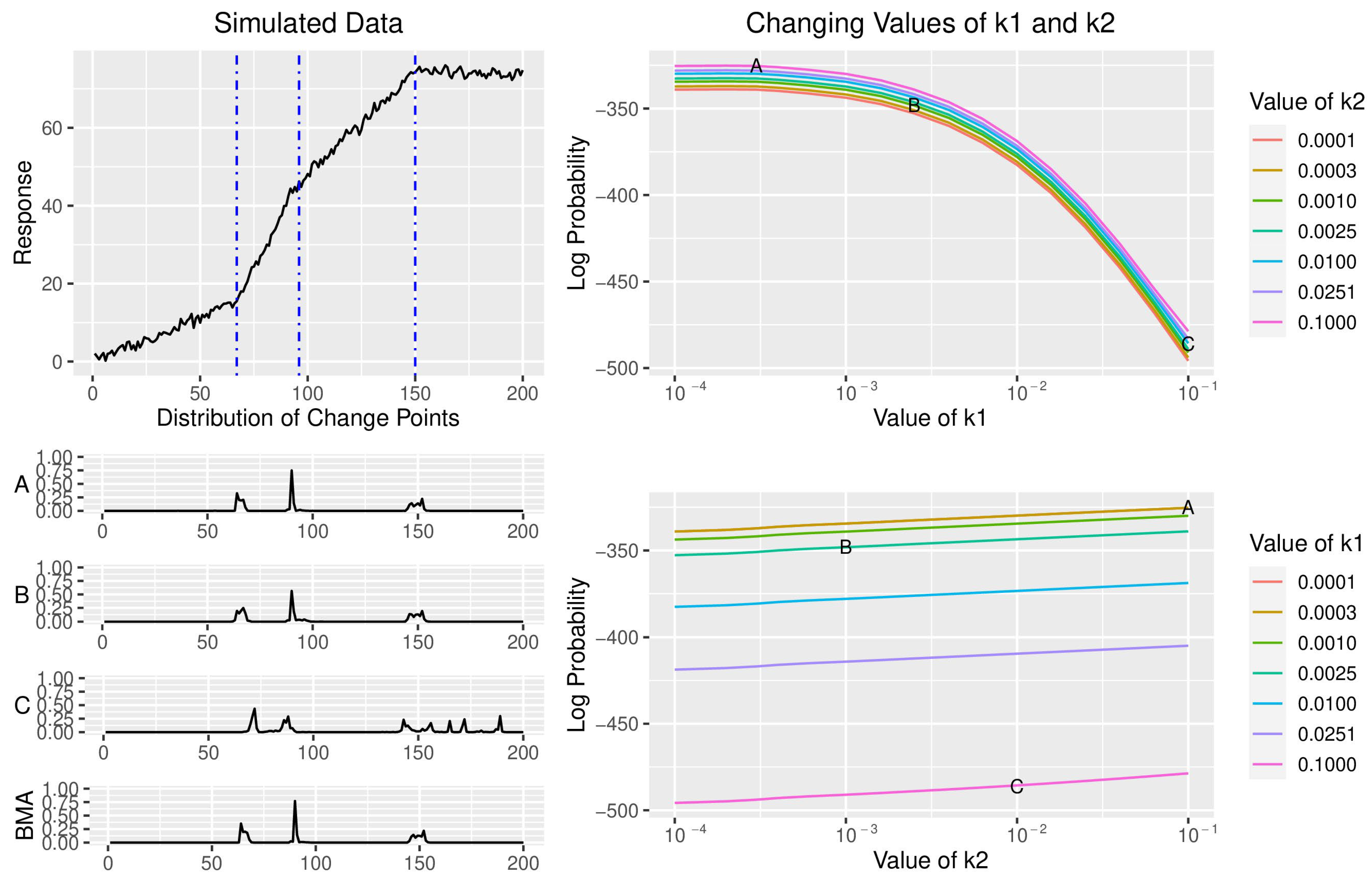
Figure 2 gives examples of “good” and “bad” choices for the prior parameters using a simulated dataset generated according to the process outlined in Section 3.1. Notice that when a poor choice for the parameter values is made, the model can infer either too few or too many change points, while a “good” set of parameters allows for a proper inference. It is easy to see what makes a “good” and “bad” choice of parameters on a simulated dataset where the locations of the change points are known, but much harder when the goal is to infer the unknown location of change points on a real dataset. Fortunately, our study shows that the “good” parameters also tend to produce the most probable solutions, so we can use Bayesian Model Averaging (BMA) to marginalize out the choice of the hyperparameters and arrive at the best overall solution [56].
Define θ to be the parameters of interest and suppose that we have a set of possible models under consideration, M1, …, Mm. BMA is defined as:
P ( θ   |   Y ) = i = 1 m P ( θ | Y ,   M i ) P ( M i | Y )
In words, the posterior distribution of the parameters of interest is a weighted average of the posterior distribution of the parameters for each model, weighted by the likelihood of each model. This means that more probable models will have a stronger impact on the posterior distribution of the parameters of interest.
In this scenario, each model is defined by the chosen values of the hyperparameters k 0 = k 1 , k 2 , v 0 , and σ 0 2 . Therefore, we can equate the term “model” with a set of hyperparameters. The parameters of interest, θ, are the number and locations of the change points, along with the parameters of the regression model in each region of the data. Thus, our sampling procedure (Step 3 of the Bayesian change point algorithm), along with the use of conjugate prior distributions, makes the quantity P ( θ | Y ,   M i ) easy to evaluate. Since each model is determined by its set of parameters, the term P ( M i | Y ) tells us how good a specific set of hyperparameters is and can be obtained through one final application of Bayes’ rule:
P M i | Y = P Y | M i P M i j = 1 m P Y | M j P M j
Note that P Y | M i , the probability of the data given the model after marginalizing out the parameters of the model and the location of the change points, is calculated as part of Step 3 of the Bayesian change point algorithm. A priori, if we assume that all models (i.e., all sets of values for the hyperparameters) are equally likely, this expression reduces to:
P M i | Y = P Y | M i j = 1 m P Y | M j
In the simulations that follow, we vary the values of k 0 = k 1 , k 2 , v 0 , and σ 0 2 to determine the posterior distribution of each model and then combine this information with that model’s distribution of change point locations to obtain the “model averaged” solution. The process is conceptually simple, but computationally intensive.

3.2.1. Changing the Values of k1 and k2

For this analysis, we generated a dataset according to the process outlined in Section 3.1 (Figure 3), assuming ρ = 0.25 and a noise level of 1. Values of v0 and σ 0 2 are both fixed at 1 (i.e., one prior observation for the variance equal to 1). Here, we are interested in studying values of k1 and k2 between 10−4 and 10−1, so we choose 16 equally spaced values for each parameter on the log10 scale. Figure 3 displays how the log probability of the data changes as we vary the values of k1 and k2 and the posterior distribution of change point locations for three sets of values of k1 and k2 (labeled A, B, and C). As the value of k1 increases from 0.0001 to 0.1 (moving from point A to B to C), the log probability of the data decreases, while changing the value of k2 from 0.001 to 0.1 (compare points A and B) does not have a significant impact on the log probability of the data. For this particular dataset, a small value of k1 is necessary because it allows the intercept of the model to be significantly larger than the residual variance. Forcing the intercept to take on a small value also introduces a number of spurious change points, as we limit the set of potential regression parameters in each interval. Notice that points A and B have a relatively similar log probability, and show only subtle differences in their distribution of change point locations, whereas point C has a much lower log probability and a significantly different distribution of change points.

3.2.2. Changing the Values of v0 and σ 0 2

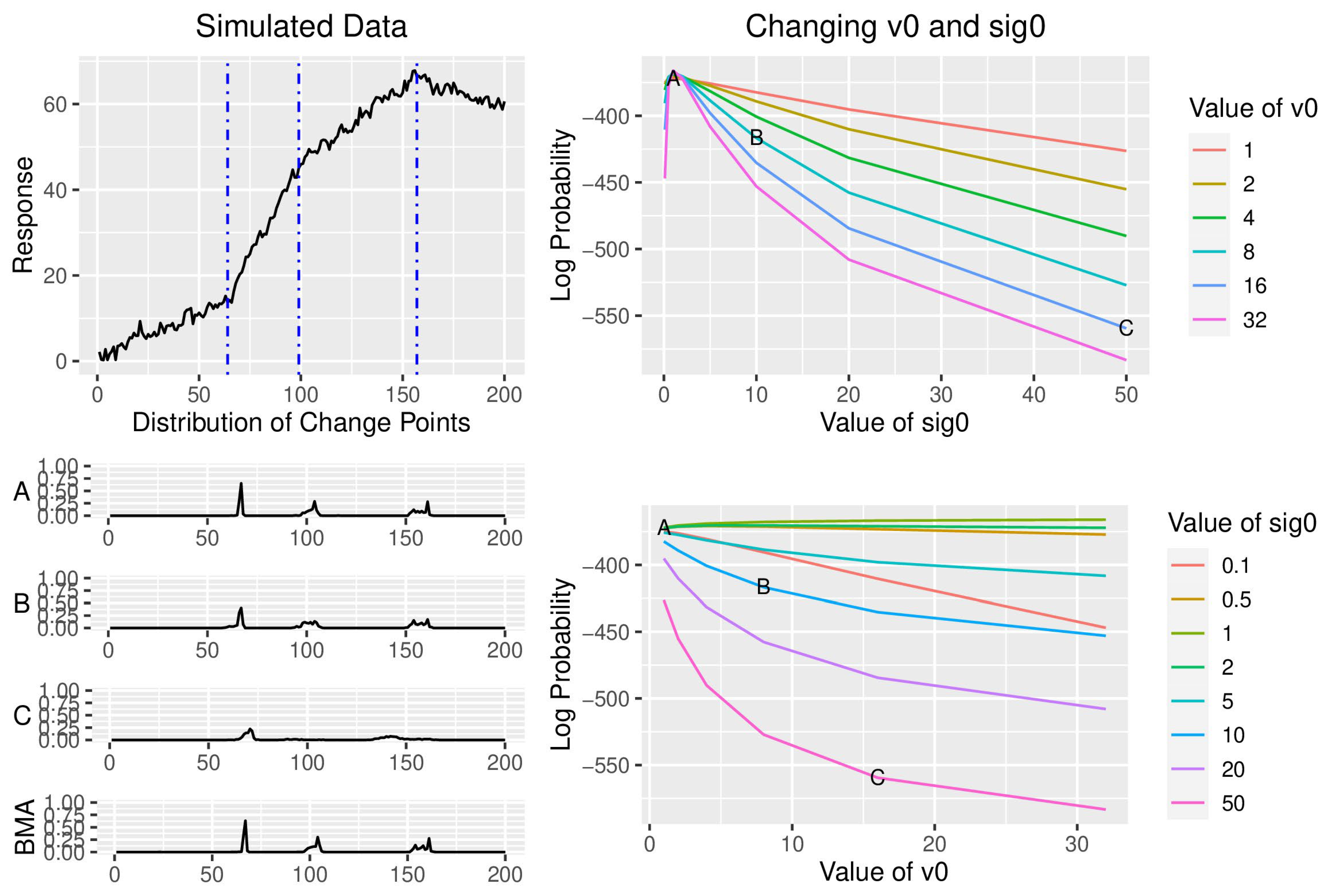
We again generated a dataset according to the process outlined in Section 3.1 (Figure 4), assuming ρ = 0.25 and a noise level of 1. For this analysis, values of k1 and k2 are fixed at 0.001. Here, we study how values of v0 and σ 0 2 affect the inference, so we choose v0 = 1, 2, 4, 8, 16, and 32, and values of σ 0 2 = 0.1, 0.5, 1, 2, 5, 10, 20, and 50. The calculation required for Step 1 of the Bayesian change point algorithm calculates a quantity analogous to a posterior sum or squares, which is the sum of the prior variability, v 0 σ 0 2 , the variability of the regression parameters, and the residual sum of squares. When a change point is introduced into the model, this term appears twice (once for each region of the data), so a larger value of the product v 0 σ 0 2 creates a barrier against additional change points. As we move from points A to B to C in Figure 4, this product increases, resulting in a posterior distribution with fewer detected change points. The locations of the change points are not altered, only our confidence in their existence. In addition, the value of v0 does not affect the log probability of a model if we choose values of σ 0 2 similar to the actual residual variance (e.g., 0.5, 1, and 2), which is consistent with their interpretation as prior observations of the residual variance. On the other hand, choosing larger values of v 0 will quickly decrease the log probability of the model if the chosen value of σ 0 2 is inconsistent with the data. As a result, we always recommend choosing v 0 = 1, so that our prior distribution on the error variance has a minimal impact on the posterior inference.

3.2.3. Applying BMA

Figure 3 and Figure 4 show that the models of lower probability (i.e., those with a “bad” choice of values for the hyperparameters) often do not have the correct number of change points, inferring either too few or too many change points. Fortunately, BMA lets us keep all the benefits of a Bayesian solution to the multiple change point problem, in particular the uncertainty bounds on the number and locations of change points, while also helping to prevent a “bad” choice of hyperparameters. Here, the models weighted most heavily are those with the highest probability, which also tend to infer the correct number of change points. Figure 3 and Figure 4 show the BMA solution to each simulation, which looks most similar to point A in each figure, the most probable of the three models shown for each simulation. This nicely illustrates how BMA can help to eliminate the effects of a “bad” choice of values for the hyperparameters.

4. Applications to Climate Data

4.1. Pacific Decadal Oscillation a Change in Mean

Pacific Decadal Oscillation (PDO) was first identified in the late 1990s [57] and describes sea surface temperature anomalies over the northeastern Pacific Ocean. Similar to El Niño/Southern Oscillation (ENSO), PDO oscillates between two states (positive and negative) that are correlated with by widespread variations in the Pacific Basin and North American climate [58]. The positive phase is characterized by cooler sea surface temperatures north of Hawaii and warmer than normal sea surface temperatures along the western coast of North America. The reverse is true in a negative phase. However, unlike ENSO, PDO is an aggregation of several independent processes rather than just a single climate phenomenon and the positive/negative phases can last for 20–30 years [59]. Researchers also believe that PDO can intensify or diminish the impacts of ENSO depending on whether or not they are in the same phase. If both ENSO and the PDO are in the same phase, then the impacts of El Niño/La Nina may be magnified. Conversely, if they are out of phase, then the effects may offset each other resulting in a milder ENSO event [60]. More information about PDO can be found in [61].
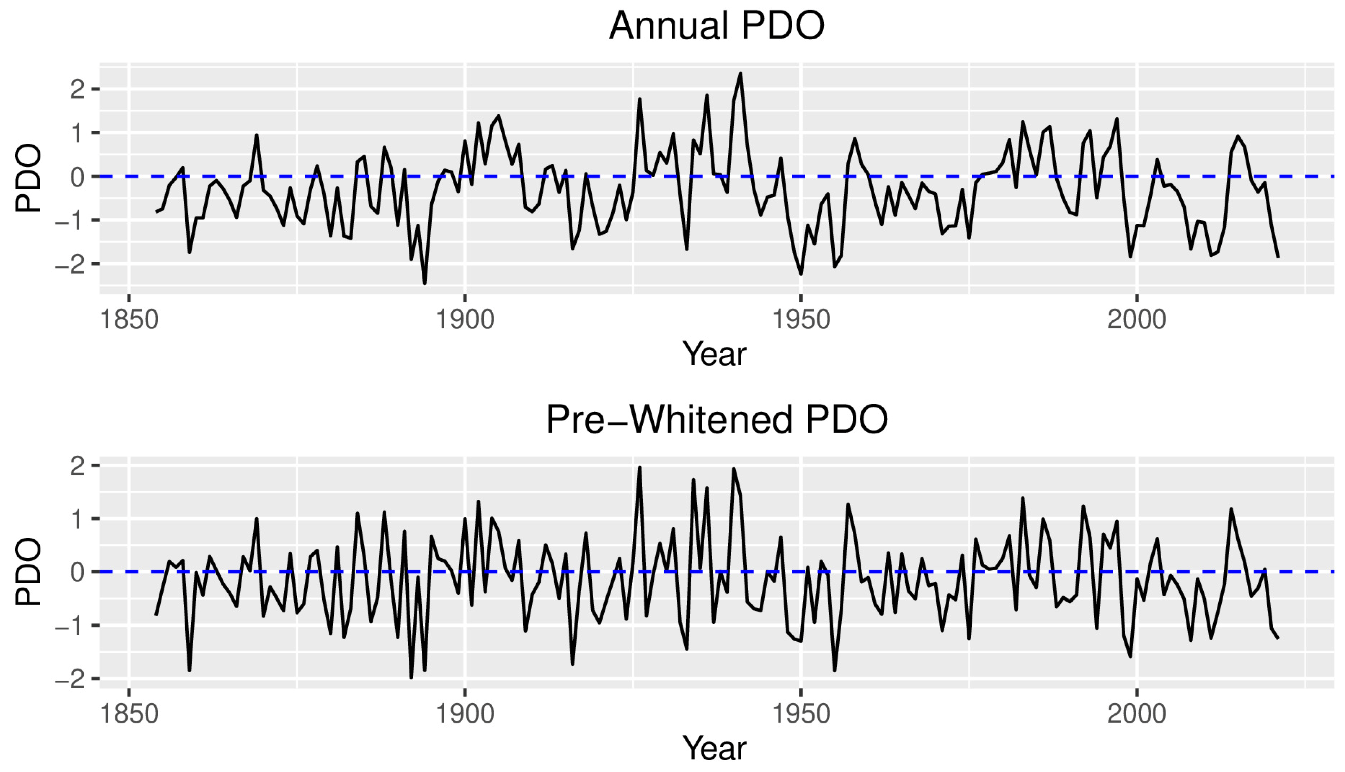
The PDO dataset can be downloaded from the National Centers for Environmental Information website (https://www.ncei.noaa.gov/access/monitoring/pdo/, accessed 15 August 2022). Annual means from 1854 to 2021 were calculated from monthly values for each year (Figure 5). This dataset has been previously analyzed for change points by other researchers (e.g., [12,47,57,62]), so it represents an interesting application of the approach described in this paper. Here, our goal is to fit a piecewise constant model to the PDO where the change points represent transitions between the positive and negative phases of PDO.
The autocorrelation function (R function acf()) shows that the residuals in the PDO are correlated, so we begin our analysis with the pre-whitening technique described in Section 3.1 to help eliminate change points due to autocorrelation rather than a change in the phase of the PDO. For our analysis, we set the value of m to be 8, since the positive and negative PDO phases are expected to last 20–30 years (l was chosen as 25). Following the procedure outlined in Section 3.1, we calculate p ^ = 0.155 , and the bias-corrected estimate of the first-order autocorrelation as p ^ c = 0.53 (consistent with 0.46 in [47], who studied a shorter time series), which is near the point at which false positive change points become a regular part of the inference (Table 1). At this point, the autocorrelation function shows no significant correlation in the residuals, so we can continue with change point analysis.
After pre-whitening, we set v0 = 1, and then allowed potential values of k1 and σ 0 2 to be the same as in Section 3.2. BMA was then used to accumulate these models to produce a single inference on the number and location of change points in the PDO data. The Bayesian change point algorithm does not detect any change points in the PDO. This result is surprising considering all the discussion of positive (e.g., 1925 to 1947 and 1976 to 1999) and negative phases (e.g., 1946 to 1976) of the PDO (see for example [57]), but consistent with the results of [12], who also identified a constant mean plus AR(1) model as the best fitting model for the PDO. This is not to say that positive and negative phases of the PDO do not exist—just that their magnitude and/or duration are not substantial enough to warrant the placement of a change point by either the Bayesian change point model or PELT [12].
Note that if we had instead analyzed the monthly rather than mean annual PDO values, the autocorrelation is much higher ( ρ = 0.855). An autocorrelation this high will induce a large number of spurious change points if the model does not have an autoregressive component (Table 1). After pre-whitening the monthly PDO data, the Bayesian change point algorithm did not detect any change points (results not shown).

4.2. Global Surface Temperature Anomalies—A Change in Trend

The Earth’s temperature has risen by an average of 0.14° Fahrenheit (0.08° Celsius) per decade since 1880, but the rate of warming has not been consistent over time. In fact, the rate of warming since 1981 is 0.32 °F (0.18 °C), more than twice the long-term average. This past year was the sixth-warmest on record (0.84 °C above the 20th century average), and the years 2013–2021 are nine of the ten warmest years on record [63,64]. Since the rate of warming fluctuates over time, a change point model with a linear trend seems most appropriate to model global surface temperature data.
Although surface temperature data are collected at stations across the globe, absolute temperature measurements can be difficult to take in certain geographic locations. Thus, temperature anomalies, or the departure from a reference value, are used instead and allow for a more effective and reliable comparison between different geographic locations. A global surface temperature anomalies dataset attempts to combine this temperature information into a measure of global surface temperatures. Several groups have created global surface temperature anomalies datasets, all with slightly different assumptions. One such time series is the HadCRUT5 dataset produced by the Met Office Hadley Centre [65], which begins in 1850 and has a reference period of 1961–1990. The data can be downloaded from https://www.metoffice.gov.uk/hadobs/hadcrut5/. Two others are MLOST, NOAA’s Merged Land Ocean Global Surface Temperature Analysis Dataset (NOAA) [66], available at (https://www.ncei.noaa.gov/access/monitoring/global-temperature-anomalies/anomalies, accessed 15 August 2022), which starts in 1880 and has a reference period of 1901–2000, and GISTEMP, NASA’s Goddard Institute for Space Studies Surface Temperature Analysis ([67], available at https://data.giss.nasa.gov/gistemp/, accessed 15 August 2022), which starts in 1880 and has a reference period of 1951–1980. The University Corporation for Atmospheric Research website (https://climatedataguide.ucar.edu/, accessed 15 August 2022) contains additional information on these and several related datasets.
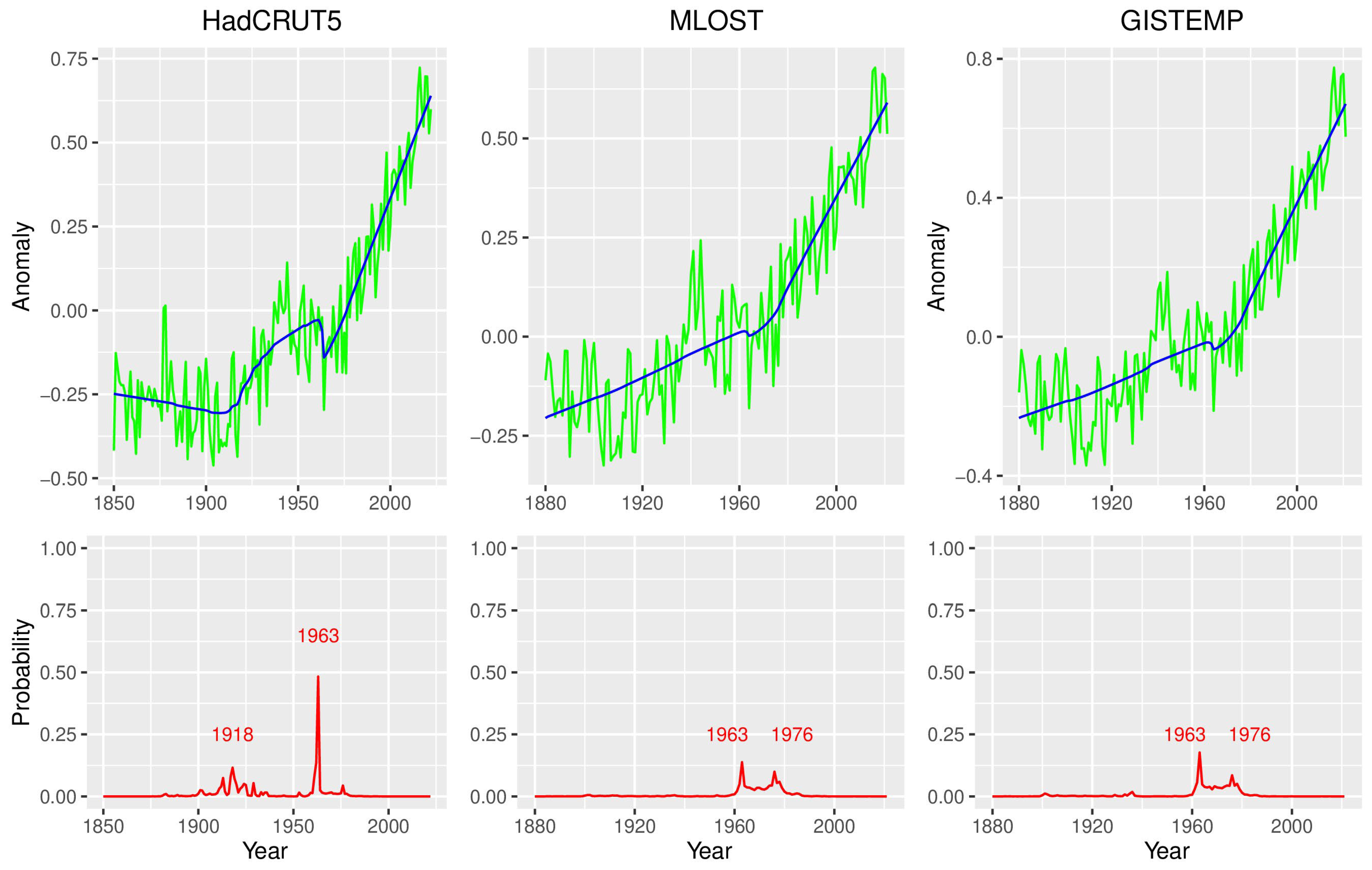
As with the PDO data, the autocorrelation function was used to initially check for correlated residuals and then to verify that the pre-whitening technique was effective. For this analysis, we expect up to 4 change points across the 140-year record, so we set the value of m to be 12. Following the procedure outlined in Section 3.1, we calculate p ^ = 0.154 , and the bias-corrected estimate of the first-order autocorrelation as p ^ c = 0.336, which is small enough so as to not have a major impact on the inference (Table 2). Nevertheless, we pre-whitened the data to help eliminate any change points that may arise due to autocorrelation. As with the PDO data, we set v0 = 1, and then allowed the values of k1 and k2 to vary as in Section 3.2. Since the variance of the temperature anomaly datasets is so small (<0.1 after pre-whitening), we chose potential values for σ 0 2 = 0.05, 0.1, 0.5, 1, 2, 5, 10, and 20. BMA was then used to accumulate these models to produce a single inference on the number and location of change points in the three temperature anomaly datasets.
The Bayesian change point model with BMA detected only a single change point in the MLOST and GISTEMP datasets, and two change points in the HadCRUT5 data (Figure 6). This result is somewhat surprising and includes fewer change points than previous analyses (e.g., [68]). However, the authors note that these datasets are continually revised and updated. Repeating the analysis of [68] on the revised datasets using the same parameter values now produces an inference with fewer change points, so in that sense, the results are consistent with previous studies on the same dataset.

5. Discussion

This paper addresses two open questions related to the Bayesian change point model of [37], namely, how autocorrelation and the choice of values for the hyperparameters can affect the inference. When a change point model is used to analyze real data, the “true” number of change points is generally unknown. As a result, it is hard to know whether a model is giving accurate and precise results. To see how our model performs in difference scenarios, simulated data were generated which varied the number and location of change points, the regression coefficients in each section of the data, the variance of the residual error, and the magnitude of autocorrelation. Any change that reduces the signal-to-noise ratio of the dataset (e.g., larger values of ρ or σ2, subtle changes in the regression parameters, etc.) makes change points harder to detect, and thus has an impact on the accuracy of the model. Specifically, a smaller signal-to-noise ratio manifests itself in the posterior distribution as greater uncertainty in the location of a change point or a complete lack of detection by the algorithm.
Autocorrelation is often present in real data, yet [37] assumes that the error terms are independent, mean 0, normally distributed random variables. Simulations show that the inference made by the Bayesian change point model is not strongly affected by low levels of first-order autocorrelation ( ρ < 0.5, see Table 1 and Table A1)—the algorithm is still able to detect the correct number of change points in the data. However, when the first-order autocorrelation is larger, it can create a similar pattern to that of a change in the mean or long-term trend (46–48), which can shift the inferred location of true change points (if the autocorrelation makes the pattern appear to start earlier or later than it actually does) and introduce spurious change points. To counter the effect of serial correlation, we pre-whiten the data using the Cochrane–Orcutt method with a bias-corrected estimate of the first-order autocorrelation. Results show that pre-whitening the data eliminates the spurious change points introduced by the autocorrelation. However, pre-whitening the data reduces the magnitude of the shift between adjacent segments, making true change points harder to detect. This is partially offset by a reduction in the variance, but not completely [47]. Both of our applications (PDO and global surface temperature anomalies) exhibit only first-order autocorrelation, so we did not study how the pre-whitening approach would fare on data with higher-order autocorrelation.
As with any Bayesian analysis, the inference can be sensitive to the choice of the prior distribution. In this case, we use conjugate priors for both the regression parameters and the error variance, so the subjectivity comes in through the values of the hyperparameters for these two distributions. As seen in Figure 3 and Figure 4, changing the values of the hyperparameters generally affects the inferred number of change points, but not their location. In other words, we can think of the changing values of the hyperparameters as creating more or less stringent criteria for the algorithm to “detect” a change point. A “bad” choice of values for the hyperparameters can produce an inference with too few or too many inferred change points (Figure 2). To avoid this problem, we propose a BMA technique to weight each model’s inference by the posterior probability of that model, so that “good” parameter choices (as defined by the posterior probability of the model) carry more weight than “bad” parameter choices. The result is an inference that takes into account multiple different potential sets of hyperparameters.
BMA partially eliminates the problem of the model being sensitive to the values of the hyperparameters. The problem is only partially eliminated because BMA is being conducted using only a finite set of potential values for the hyperparameters rather than considering all possible values. A Monte Carlo approach would fix this issue but at an increased computational cost. Since models (defined by the set of values of the hyperparameters) of similar probability tend to produce a similar inference (see the similarity of change point solutions for points A and B in Figure 3), and the model itself is not especially sensitive to small changes in parameters values, we did not feel that this increased computational burden would significantly improve our BMA solutions. The interested researcher could also try placing a non-uniform prior over the set of values for the hyperparameters if they believe certain values to be more likely than others.
A major limitation of the Bayesian change point model discussed in this paper is its run time, which can make BMA over a large parameter space prohibitive. Computational complexity is a common challenge for Bayesian methods, so this limitation is not unique to our model. However, we find inference produced by the Bayesian change point algorithm to be reliable and believe that the reduced subjectivity afforded by BMA to be an important step towards letting the data dictate which model is “best”. Future research should focus on analyzing the impact that the range of parameter values has on the inference and on further reducing the compute time so that this approach can be applied to longer and more complex datasets.

Author Contributions

Both authors contributed equally to all aspects of this project. All authors have read and agreed to the published version of the manuscript.

Funding

This research received no external funding.

Data Availability Statement

R code to run the Bayesian Change Point algorithm and associated datasets can be obtained by contacting the corresponding author, [email protected].

Acknowledgments

The authors would like to thank the Weiss Summer Research Program at the College of the Holy Cross for providing funding to support this project.

Conflicts of Interest

The authors declare no conflict of interest.

Appendix A. Correcting for Autocorrelation in the Presence of a Linear Trend Model

A second study was conducted to analyze how autocorrelation affects the Bayesian change point algorithm’s ability to detect change points when none actually exist. Here, we consider a linear model with no change points ( Y = 4 + 0.05 X + ϵ ). An auto-regressive signal of level ρ = 0.1, 0.2, 0.3, …, 0.9 is then generated using the R function arima.sim() and added to each dataset (a total of 10,000 simulations for each of the two models). The value of m is chosen to be 20, k0 = (0.01, 0.01), v0 = 1, σ 0 2 = 1, dmin = 5, and kmax = 20. Since the goal of this simulation is to see how autocorrelation affects the inference, optimizing these parameters is not critical. The Bayesian change point model calculates the posterior distribution of the number of change points for each dataset, which can be used to determine the expected number of change points in the dataset. Table A1 gives the average number of detected change points across the 1000 simulated datasets for each value of ρ before and after pre-whitening, along with the number of datasets where the algorithm correctly identified zero change points. As with Table 1, it is clear from these data that pre-whitening can help to eliminate spurious change points that arise from autocorrelation.
Table A1. Autocorrelation in a Linear Trend Model. A total of 1000 datasets were generated for each value of the autocorrelation parameter, ρ , for a model that includes a linear trend. The average number of change points detected by the Bayesian change point model before and after pre-whitening is indicated for each value of ρ , along with the number of datasets (out of 1000) where the algorithm correctly identified zero change points (i.e., the number of datasets where the expected number of change points <0.5). Note that a value of ρ = 0 corresponds to white noise.
ρ00.10.20.30.40.50.60.70.80.9
Data with AutocorrelationEstimated ρ ^ c N/A0.0390.1390.2290.3210.4190.5010.5910.6660.732
Change Points Detected<10−3<10−3<10−3<10−30.0030.0130.0870.4721.8613.577
# Correct100010001000100099899092870020318
Pre-WhitenedChange Points DetectedN/A<10−3<10−3<10−3<10−3<10−30.0020.0150.0800.450
# CorrectN/A10001000100010001000998989940693
For the linear trend model (Table A1), we estimate the value of the autoregressive parameter on the residuals of the model after accounting for the linear trend. The fact that we underestimate the value of the autocorrelation should not be surprising. Both [69] and [70] discuss the difficulty of jointly estimating the trend and autoregressive parameters of a model as they are highly interdependent. Note that if we estimated the value of ρ based on the entire dataset rather than short subsegments of the data, then the estimated value of ρ is much closer to the true value of ρ (results not shown). However, this approach is problematic in the presence of the change points.

References

  1. Wurtz, D.; Chalabi, Y.; Setz, T. New Directions in Active Portfolio Management: Stability Analytics, Risk Parity, Rating and Ranking, and Geometric Shape Factors; ETH Econophysics Working and White Papers Series; Rmetrics: Zurich, Switzerland, 2013; p. 3. [Google Scholar]
  2. Thies, S.; Molnár, P. Bayesian change point analysis of Bitcoin returns. Financ. Res. Lett. 2018, 27, 223–227. [Google Scholar] [CrossRef]
  3. Chopin, N. Dynamic detection of change points in line time series. Ann. Inst. Stat. Math. 2007, 59, 349–366. [Google Scholar] [CrossRef]
  4. Barnett, I.; Onnela, J.P. Change Point Detection in Correlation Networks. Sci. Rep. 2016, 6, 18893. [Google Scholar] [CrossRef] [Green Version]
  5. Western, B.; Kleykamp, M. A Bayesian Change Point Model for Historical Time Series Analysis. Political Anal. 2004, 12, 354–374. [Google Scholar] [CrossRef]
  6. Robinson, L.F.; Wager, T.D.; Lindquist, M.A. Change point estimation in multi-subject fMRI studies. Neuroimage 2010, 49, 1581–1592. [Google Scholar] [CrossRef] [Green Version]
  7. Chen, G.; Lu, G.; Shang, W.; Xie, Z. Automated Change-Point Detection of EEG Signals Based on Structural Time-Series Analysis. IEEE Access 2019, 7, 180168–180180. [Google Scholar] [CrossRef]
  8. Kass-Hout, T.A.; Xu, Z.; McMurray, P.; Park, S.; Buckeridge, D.L.; Brownstein, J.S.; Finelli, L.; Groseclose, S.L. Application of change point analysis to daily influenza-like illness emergency department visits. J. Am. Med. Inform. Assoc. 2012, 19, 1075–1081. [Google Scholar] [CrossRef] [PubMed] [Green Version]
  9. Ruggieri, E.; Herbert, T.; Lawrence, K.T.; Lawrence, C.E. Change point method for detecting regime shifts in paleoclimatic time series: Application to d18O time series of the Plio-Pleistocene. Paleoceanography 2009, 24, PA1204. [Google Scholar] [CrossRef] [Green Version]
  10. Gallagher, C.; Lund, R.; Robbins, M. Changepoint detection in daily precipitation data. Environmetrics 2012, 23, 407–419. [Google Scholar] [CrossRef]
  11. Kim, C.; Suh, M.; Hong, K. Bayesian Changepoint Analysis of the Annual Maximum of Daily and Subdaily Precipitation over South Korea. J. Clim. 2009, 22, 6741–6757. [Google Scholar] [CrossRef]
  12. Beaulieu, C.; Killick, R. Distinguishing trends and shifts from memory in climate data. J. Clim. 2018, 31, 9519–9543. [Google Scholar] [CrossRef]
  13. Kendrick, L.; Musial, K.; Gabrys, B. Change point detection in social networks—Critical review with experiments. Comput. Sci. Rev. 2018, 29, 1–13. [Google Scholar] [CrossRef]
  14. Desobry, F.; Davy, M.; Doncarli, C. An online kernel change detection algorithm. IEEE Trans. Signal Process. 2005, 53, 2961–2974. [Google Scholar] [CrossRef]
  15. Liu, J.S.; Lawrence, C.E. Bayesian Inference on Biopolymer Models. Bioinformatics 1999, 15, 38–52. [Google Scholar] [CrossRef] [PubMed] [Green Version]
  16. Maidstone, R.; Hocking, T.; Rigaill, G.; Fearnhead, P. On optimal multiple change-point algorithms for large data. Stat. Comput. 2017, 27, 519–533. [Google Scholar] [CrossRef] [Green Version]
  17. Aminikhanghahi, S.; Cook, D.J. A survey of methods for time series change point detection. Knowl. Inf. Syst. 2017, 51, 339–367. [Google Scholar] [CrossRef] [Green Version]
  18. Chen, J.; Gupta, A.K. Parametric Statistical Change Point Analysis; Birkhauser: New York, NY, USA, 2012. [Google Scholar] [CrossRef]
  19. Page, E.S. Continuous Inspection Schemes. Biometrika 1954, 41, 100–115. [Google Scholar] [CrossRef]
  20. Page, E. A test for a change in a parameter occurring at an unknown point. Biometrika 1955, 42, 523–527. [Google Scholar] [CrossRef]
  21. Zeileis, A.; Leisch, F.; Hornik, K.; Kleiber, C. strucchange: An R Package for Testing for Structural Change in Linear Regression Models. J. Stat. Softw. 2002, 7, 1–38. [Google Scholar] [CrossRef] [Green Version]
  22. Hawkins, D.M.; Qiu, P.; Kang, C.W. The Changepoint Model for Statistical Process Control. J. Qual. Technol. 2003, 35, 355–366. [Google Scholar] [CrossRef]
  23. Kawahara, Y.; Sugiyama, M. Change-point detection in time-series data by direct density-ratio estimation. In Proceedings of the 2009 SIAM International Conference on Data Mining, Sparks, NV, USA, 30 April–2 May 2009; Society for Industrial and Applied Mathematics: Philadelphia, PA, USA, 2009; pp. 389–400. [Google Scholar] [CrossRef] [Green Version]
  24. Ross, G.J. Parametric and Nonparametric Sequential Change Detection in R: The cpm Package. J. Stat. Softw. 2015, 66, 1–20. [Google Scholar] [CrossRef] [Green Version]
  25. Scott, A.J.; Knott, M. A Cluster Analysis Method for Grouping Means in the Analysis of Variance. Biometrics 1974, 30, 507–512. [Google Scholar] [CrossRef] [Green Version]
  26. Shi, X.; Gallagher, C.; Lund, R.; Killick, R. A comparison of single and multiple changepoint techniques for time series data. Comput. Stat. Data Anal. 2022, 170, 107433. [Google Scholar] [CrossRef]
  27. Olshen, A.B.; Venkatraman, E.; Lucito, R.; Wigler, M. Circular binary segmentation for the analysis of array-based DNA copy number data. Biostatistics 2004, 5, 557–572. [Google Scholar] [CrossRef] [PubMed]
  28. Fryzlewicz, P. Wild binary segmentation for multiple change-point detection. Ann. Stat. 2014, 42, 2243–2281. [Google Scholar] [CrossRef]
  29. Auger, I.E.; Lawrence, C.E. Algorithms for the Optimal Identification of Segment Neighborhoods. Bull. Math. Biol. 1989, 51, 39–54. [Google Scholar] [CrossRef]
  30. Bai, J.; Perron, P. Computation and Analysis of Multiple Structural Change Models. J. Appl. Econom. 2003, 18, 1–22. [Google Scholar] [CrossRef] [Green Version]
  31. Killick, R.; Fearnhead, P.; Eckley, I.A. Optimal Detection of Changepoints With a Linear Computational Cost. J. Am. Stat. Assoc. 2012, 107, 1590–1598. [Google Scholar] [CrossRef]
  32. Barry, D.; Hartigan, J.A. A Bayesian Analysis for Change Point Problems. J. Am. Stat. Assoc. 1993, 88, 309–319. [Google Scholar] [CrossRef]
  33. Carlin, B.P.; Gelfand, A.E.; Smith, A.F.M. Hierarchical Bayesian analysis of changepoint problems. Appl. Stat. 1992, 41, 389–405. [Google Scholar] [CrossRef]
  34. Green, P.J. Reversible jump Markov chain Monte Carlo computation and Bayesian model determination. Biometrika 1995, 82, 711–732. [Google Scholar] [CrossRef]
  35. Fearnhead, P. Exact and Efficient Bayesian Inference for Multiple Changepoint problems. Stat. Comput. 2006, 16, 203–213. [Google Scholar] [CrossRef] [Green Version]
  36. Whiteley, N.; Andrieu, C.; Doucet, A. Bayesian Computational Methods for Inference in Multiple Change-Point Models. 2011. Available online: http://www.maths.bris.ac.uk/~manpw/change_points_2011.pdf (accessed on 20 June 2022).
  37. Ruggieri, E. A Bayesian Approach to Detecting Change Points in Climatic Records. Int. J. Climatol. 2013, 33, 520–528. [Google Scholar] [CrossRef]
  38. Adams, R.P.; MacKay, D.J.C. Bayesian Online Changepoint Detection. 2007. Available online: http://arxiv.org/pdf/0710.3742.pdf (accessed on 20 June 2022).
  39. Fearnhead, P.; Clifford, P. On-line inference for hidden Markov models via particle filters. J. R. Stat. Soc. Ser. B 2003, 65, 887–899. [Google Scholar] [CrossRef]
  40. Fearnhead, P.; Liu, Z. On-line inference for multiple changepoint problems. J. R. Stat. Soc. Ser. B 2007, 69, 589–605. [Google Scholar] [CrossRef] [Green Version]
  41. West, M.; Harrison, J. Bayesian Forecasting and Dynamic Models, 2nd ed.; Springer: New York, NY, USA, 1997. [Google Scholar]
  42. Zhang, Y.M.; Wang, H.; Bai, Y.; Mao, J.X.; Chang, X.Y.; Wang, L.B. Switching Bayesian dynamic linear model for condition assessment of bridge expansion joints using structural health monitoring data. Mech. Syst. Signal Process. 2021, 160, 107879. [Google Scholar] [CrossRef]
  43. Ruggieri, E. A Pruned, Recursive Solution to the Multiple Change Point Problem. Comput. Stat. 2018, 33, 1017–1045. [Google Scholar] [CrossRef]
  44. Ruggieri, E.; Antonellis, M. An exact approach to Bayesian sequential change point detection. Comput. Stat. Data Anal. 2016, 97, 71–86. [Google Scholar] [CrossRef] [Green Version]
  45. Hasselmann, K. Stochastic climate models Part I. Theory. Tellus 1976, 28, 473–485. [Google Scholar] [CrossRef] [Green Version]
  46. von Storch, H. Misuses of statistical analysis in climate research. In Analysis of Climate Variability; Springer: Berlin/Heidelberg, Germany, 1999; pp. 11–26. [Google Scholar]
  47. Rodionov, S.N. Use of prewhitening in climate regime shift detection. Geophys. Res. Lett. 2006, 33, L12707. [Google Scholar] [CrossRef] [Green Version]
  48. Shi, X.; Beaulieu, C.; Killick, R.; Lund, R. Changepoint Detection: An Analysis of the Central England Temperature Series, J. Clim. 2022, 35, 2729–2742. [Google Scholar] [CrossRef]
  49. Lund, R.; Wang, X.L.; Lu, Q.Q.; Reeves, J.; Gallagher, C.M.; Feng, Y. Changepoint detection in periodic and autocorrelated time series. J. Clim. 2007, 20, 5178–5190. [Google Scholar] [CrossRef] [Green Version]
  50. Chatfield, C. The Analysis of Time Series: An Introduction, 7th ed.; Chapman & Hall/CRC Press: Boca Raton, FL, USA, 2003. [Google Scholar]
  51. Beaulieu, C.; Chen, J.; Sarmiento, J.L. Change-point analysis as a tool to detect abrupt climate variations. Philos. Trans. R. Soc. A Math. Phys. Eng. Sci. 2012, 370, 1228–1249. [Google Scholar] [CrossRef] [Green Version]
  52. Wang, X.L. Accounting for autocorrelation in detecting mean shifts in climate data series using the penalized maximal t or F test. J. Appl. Meteor. Climatol. 2008, 47, 2423–2444. [Google Scholar] [CrossRef]
  53. Serinaldi, F.; Kilsby, C.G. The importance of prewhitening in change point analysis under persistence. Stoch. Environ. Res. Risk Assess. 2016, 30, 763–777. [Google Scholar] [CrossRef] [Green Version]
  54. Shaman, P.; Stine, R. The bias of autoregressive coefficient estimators. J. Am. Stat. Assoc. 1988, 83, 842–848. [Google Scholar] [CrossRef]
  55. Marriott, F.H.C.; Pope, J.A. Bias in the estimation of autocorrelations. Biometrika 1954, 41, 390–402. [Google Scholar] [CrossRef]
  56. Hoeting, J.A.; Madigan, D.; Raftery, A.E.; Volinsky, C.T. Bayesian model averaging: A tutorial (with comments by M. Clyde, David Draper and E. I. George, and a rejoinder by the authors). Statist. Sci. 1999, 14, 382–417. [Google Scholar] [CrossRef]
  57. Mantua, N.J.; Hare, S.R.; Zhang, Y.; Wallace, J.M.; Francis, R.C. A Pacific Interdecadal Climate Oscillation with Impacts on Salmon Production. Bull. Am. Meteorol. Soc. 1997, 78, 1069–1079. [Google Scholar] [CrossRef]
  58. Dutton, J. “What is the Pacific Decadal Oscillation?” World Climate Service. 2021. Available online: https://www.worldclimateservice.com/2021/09/01/pacific-decadal-oscillation/ (accessed on 25 July 2022).
  59. Zhang, Y.; Wallace, J.M.; Battisti, D.S. ENSO-like interdecadal variability: 1900–93. J. Clim. 1997, 10, 1004–1020. [Google Scholar] [CrossRef]
  60. Wang, S.; Huang, J.; He, Y.; Guan, Y. Combined effects of the Pacific Decadal Oscillation and El Niño-Southern Oscillation on Global Land Dry–Wet Changes. Sci. Rep. 2014, 4, 6651. [Google Scholar] [CrossRef] [Green Version]
  61. Mantua, N.J.; Hare, S.R. The Pacific decadal oscillation. J. Oceanogr. 2002, 58, 35–44. [Google Scholar] [CrossRef]
  62. Schwing, F.B.; Jiang, J.; Mendelssohn, R. Coherency of multi-scale abrupt changes between the NAO, NPI, and PDO. Geophys. Res. Lett. 2003, 30, 1406. [Google Scholar] [CrossRef] [Green Version]
  63. Lindsey, R.; Dahlman, L. Climate Change: Global Temperature. 2022. Available online: https://www.climate.gov/news-features/understanding-climate/climate-change-global-temperature (accessed on 22 July 2022).
  64. NOAA National Centers for Environmental Information. State of the Climate: Global Climate Report for 2021. 2022. Available online: https://www.ncdc.noaa.gov/sotc/global/202113 (accessed on 28 July 2022).
  65. Morice, C.P.; Kennedy, J.J.; Rayner, N.A.; Winn, J.P.; Hogan, E.; Killick, R.E.; Dunn, R.J.H.; Osborn, T.J.; Jones, P.D.; Simpson, I.R. An updated assessment of near-surface temperature change from 1850: The HadCRUT5 dataset. J. Geophys. Res. Atmos. 2021, 126, e2019JD032361. [Google Scholar] [CrossRef]
  66. Smith, T.M.; Reynolds, R.W.; Peterson, T.C.; Lawrimore, J. Improvements to NOAA’s historical merged land–ocean surface temperature analysis (1880–2006). J. Clim. 2008, 21, 2283–2296. [Google Scholar] [CrossRef]
  67. GISTEMP Team. GISS Surface Temperature Analysis (GISTEMP), Version 4. NASA Goddard Institute for Space Studies; 2022. Available online: https://data.giss.nasa.gov/gistemp/ (accessed on 28 July 2022).
  68. Yu, M.; Ruggieri, E. Change point analysis of global temperature records. Int. J. Climatol. 2019, 39, 3679–3688. [Google Scholar] [CrossRef]
  69. Canjels, E.; Watson, M.W. Estimating deterministic trends in the presence of serially correlated errors. Rev. Econ. Stat. 1997, 79, 184–200. [Google Scholar] [CrossRef]
  70. Roy, A.; Falk, B.; Fuller, W.A. Testing for trend in the presence of autoregressive error. J. Am. Stat. Assoc. 2004, 99, 1082–1091. [Google Scholar] [CrossRef]
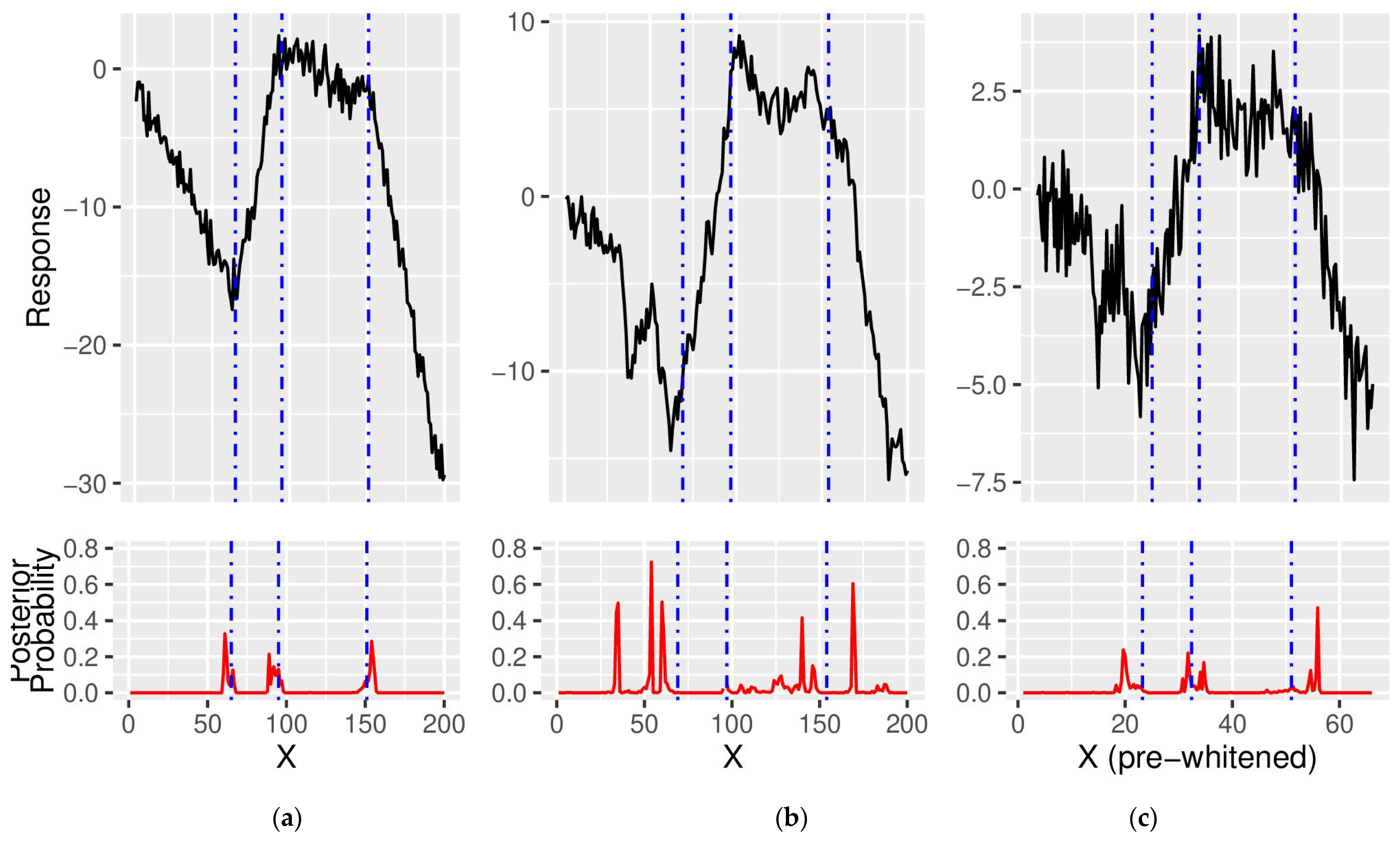
Figure 1. Detecting Change Points in the Presence of Autocorrelation. (a) A simulated dataset with 3 change points that contains only white noise. (b) Autocorrelation is added to (a) using ρ = 0.8. (c) The data in (b) after pre-whitening. The inferred location of change points is indicated below each figure, while their exact location is indicated by dotted vertical lines. Pre-whitening helps to eliminate spurious change points, but the location of the true change points becomes more difficult to correctly infer.
Mathematics 11 01082 g001
Figure 2. “Good” and “Bad” Parameter Choices. A representative dataset using the data generation process described in Section 3.1 is analyzed using different sets of values for the hyperparameters. Dotted vertical lines indicate the actual location of the change points. The left panel uses a set of parameters that produces a posterior distribution which infers too few change points while the right panel uses a set of parameters that produces a posterior distribution that infers too many change points. The middle panel correctly identifies the correct number of change points.
Mathematics 11 01082 g002
Figure 3. How k1 and k2 Affect the Posterior Distribution. The top left displays a dataset generated according to the process described in Section 3.1, along with the location of each change point, indicated as a dotted vertical line. The log probability of the data, i.e., P ( M i | Y ) , is shown on the right for various combinations of v 0 and σ 0 2 . Three sets of hyperparameters, labeled A, B, and C, are selected and their posterior distribution of the location of change points is shown in the bottom left, along with the posterior distribution for the BMA solution, which weights each solution according to its probability.
Mathematics 11 01082 g003
Figure 4. How v 0 and σ 0 2 Affect the Posterior Distribution. The top left displays a dataset generated according to the process described in Section 3.1, along with the location of each change point, indicated as a dotted vertical line. The log probability of the data, i.e., P ( M i | Y ) , is shown on the right for various combinations of v 0 and σ 0 2 . Three sets of hyperparameters, labeled A, B, and C, are selected and their posterior distribution of the location of change points is shown in the bottom left, along with the posterior distribution for the BMA solution, which weights each solution according to its probability.
Mathematics 11 01082 g004
Figure 5. Change Points in PDO. The top panel shows the annual PDO values, while the bottom panel shows a pre-whitened version of this dataset. The horizontal dotted line at 0 is for reference to help identify positive and negative phases of the PDO. The Bayesian change point algorithm did not detect any change points in this dataset.
Mathematics 11 01082 g005
Figure 6. Change Points in the Temperature Anomaly Data. The top row displays the HadCRUT5, MLOST, and GISTEMP datasets, along with the model fitted by using BMA together with the Bayesian change point model. The bottom row displays the BMA posterior distribution for the locations of change points in each dataset. HadCRUT5 has two change points detected by the model, while MLOST and GISTEMP have a bimodal distribution for a single change point.
Mathematics 11 01082 g006
Table 1. Autocorrelation in a Constant Model. A total of 1000 datasets were generated for each value of the autocorrelation parameter, ρ . The average number of change points detected by the Bayesian change point model before and after pre-whitening is indicated for each value of ρ in addition to the number of datasets (out of 1000) where the algorithm correctly identified zero change points (i.e., the number of datasets where the expected number of change points < 0.5). Note that a value of ρ = 0 corresponds to white noise.
ρ00.10.20.30.40.50.60.70.80.9
Data with AutocorrelationEstimated ρ ^ c N/A0.1010.2120.3200.4250.5210.6320.7290.8230.920
Change Points Detected0.0020.0020.0140.0270.1470.5222.0525.2918.1069.150
# Correct100010009929869217694118630
Pre-WhitenedChange Points DetectedN/A0.0020.0040.0020.0060.0040.0070.0050.0220.080
# CorrectN/A9999981000997999997998990955
Table 2. Autocorrelation in a Change Point Model with Linear Trend. A total of 1000 datasets containing a linear trend with 3 change points were generated for each value of the autocorrelation parameter, ρ . The average number of change points detected by the Bayesian change point model before and after pre-whitening is indicated for each value of ρ in addition to the true positive and perfection rate. Note that a value of ρ = 0 corresponds to white noise.
ρ 00.10.20.30.40.50.60.70.80.9
Estimated ρ ^ c N/A0.1100.2010.2890.3810.4630.5470.6240.7010.754
With AutocorrelationNumber Detected2.9972.9993.0023.0133.0533.1413.2913.7014.2735.090
True Positive Rate0.9720.9650.9560.9450.9370.8940.8380.7790.6810.596
Perfection Rate0.9220.9010.8760.8430.8290.7180.5900.4630.3360.235
After Pre-WhiteningNumber Detected N/A2.9962.9952.9932.9912.9762.9292.8552.7092.556
True Positive RateN/A0.9620.9490.9270.8920.7950.6670.5360.3540.284
Perfection RateN/A0.8970.8560.7990.7250.5200.3410.1870.0760.044
Disclaimer/Publisher’s Note: The statements, opinions and data contained in all publications are solely those of the individual author(s) and contributor(s) and not of MDPI and/or the editor(s). MDPI and/or the editor(s) disclaim responsibility for any injury to people or property resulting from any ideas, methods, instructions or products referred to in the content.